1. Introduction
As new power systems continue to advance, more prominent “double new” features, load aggregators, integrated energy systems, virtual power plants, other new ecological emergences, and network boundaries will become more complex and control services will continue to extend to the end of the line. The demand for communication channels for new power systems is growing, and the requirements for communication network coverage, operation reliability, access flexibility, and the network performance index are becoming more stringent. In addition, the role of communication in the construction of new power systems is becoming more and more important. Terminal service identification refers to the technology of identifying the application type of data stream through the features in network data packets. In the rapid development of applications and the network size of new power systems, terminal service identification has become an important part of network management and security defense. In terms of network management, terminal service identification can provide enterprises with a detailed analysis of network usage, help them understand the use of the internal network, identify network bottlenecks, optimize network performance, and improve network usage and work efficiency. In terms of network security and defense, terminal service identification can help network administrators discover and respond to abnormal traffic and malicious attacks in the network in a timely manner so as to improve the level of network security and ensure network stability and data security.
At present, in the field of service traffic identification research, especially in the field based on machine learning, the main focus is on the accuracy of service traffic identification and the accuracy of identification for a specific service, ignoring the processing capability of the actual service and whether the identification technology is applicable to various types of equipment with limited resources. For example, deep packet inspection technology is a technology that has been developed more thoroughly and has better results in practical applications, utilizing the contents of packet messages for feature string matching. However, deep packet inspection techniques require a large amount of hardware and computational power and are less effective in recognizing unknown feature strings and encrypted data streams. Therefore, it is necessary to investigate more efficient, accurate, and practical service traffic identification techniques to meet practical requirements.
Machine learning is becoming more and more popular in the field of service traffic identification due to its continuous development. Compared with traditional methods, machine learning-based algorithms can avoid the content parsing of encrypted traffic, which is a difficult problem encountered by traditional traffic classification methods. In recent years, deep packet detection based on machine learning has become a hot issue in the field of measurement [
1,
2]. According to the characteristics of the input model, service identification methods based on machine learning can be divided into two classification methods based on the data flow features and deep learning.
A power marketing audit business identification model based on K-mean clustering and text categorization was proposed in [
3]. The main idea of the qualitative analysis of the marketing work quality evaluation based on marketing results introduces, in detail, the process of constructing a qualitative analysis model of marketing quality and application examples. However, some power IoT access layer network traffic anomaly identification methods have the problem of low F1 value when facing unknown types of traffic. For this reason, Ref. [
4] designed an extreme learning machine-based network traffic anomaly identification method to power the IoT access layer to network traffic. To identify transmission segments in the power system, the shortest distance and power sensitivity index were adopted together to form a comprehensive clustering index, and then the partitioning method was used to identify transmission segments in the power system [
5]. In [
6], a large data volume P2P video streaming service was divided into small data volume units and machine learning algorithms were used to identify each data unit. Finally, the final identification result was derived by statistical weighting. A novel hybrid machine learning approach for classifying network service traffic was also proposed in [
7] which effectively recognized multi-application traffic through multi-criteria decision trees with attribute selection.
The advantage of the deep learning-based approach to service identification is that it does not have to manually extract features, eliminating the complex process of feature extraction and avoiding the loss of information entropy caused by human feature extraction. The disadvantage is that the performance of the system is largely limited by the size of the network; the large-scale network model occupies a large number of computer resources, and it is difficult to deploy in some of the first resource equipment. Deep learning-based approaches for service traffic identification typically extract the byte information of packets and convert it into a one-dimensional vector or a two-dimensional matrix to be used for model training and testing. With the outstanding feature of automatic feature extraction, the application of a deep learning to network service traffic classification has become a hot research topic. The authors of [
8] designed a two-phase network traffic classification algorithm based on the network traffic features group. The first phase in the rapid clustering and empirical attribute selection was based on the idea of the coarse classification of network data traffic. The second phase involved the use of an integrated learning approach on the first phase of the classification of a subset of fine-grained identification. The experimental results showed that the two-phase recognition algorithm could effectively improve the recognition accuracy and recognition time used. A lightweight deep learning-based business recognition framework [
9] can cope well with the problem of recognizing encrypted traffic and requires fewer storage resources. The authors of [
10] designed a deep learning model to cope with encrypted mobile application traffic which required only the first few packet payloads to complete the recognition. In addition, a CNN-based encrypted traffic algorithm [
11] converted the traffic data into a two-dimensional image format and employed an image classification algorithm to identify business traffic, providing better classification results with a 99.7% accuracy compared to the method using a one-dimensional vector data format.
As the performance of computer hardware improves, more and more research is focusing on deep neural networks, which have been found to extract richer and more abstract semantic information. However, as the size of the network increases, the training of neural networks becomes more difficult because the gradient vanishing problem may occur. To solve this problem, researchers have proposed techniques such as residual networks. In addition, there are a large number of redundant parameters in large-scale deep neural networks which require more storage and computational resources. With the popularity of embedded devices, how to deploy efficient and accurate service recognition systems on such devices with limited arithmetic and resources is also a pressing issue for researchers.
In order to address the problem of deep neural networks consuming large amounts of memory and energy in deployment and prediction, researchers have proposed a variety of parameter compression methods which are broadly categorized into the following categories, quantization, factorization, network pruning, and knowledge distillation.
Network pruning refers to reducing the computational effort of a network model by removing redundant parameters from the network, thus improving the inference speed and generalization ability of the network. In convolutional neural networks, network pruning is often used to reduce the storage space and computational resource consumption of the model. Combining quantization and pruning can further reduce the storage space and computational resource requirements. HashedNet [
12] is a method that randomly groups network connections into hash buckets and shares the weights between connections in the same hash bucket. However, the sparsely connected approach does not necessarily improve the inference speed, so the method of cropping complete convolutional templates instead of cropping individual connections has become a hot research topic. This approach enables dense matrix multiplication without the use of sparse convolutional libraries. In addition, the algorithm combining quantization and pruning can further reduce the demand for storage space and network computational resources [
13], in which the size of VGG-16 can be reduced by a factor of three from 49 MB to 552.11 MB without a loss of accuracy. It should be noted that for some application scenarios with high accuracy requirements, network pruning and quantization can lead to the problem of accuracy loss. However, several studies have used structured sparse training strategies [
14,
15] which effectively improve the operation speed of the network and reduce the dependence on hardware devices. These strategies can be pruned according to the sparsity while maintaining the structural integrity of the network and avoiding the loss of accuracy.
Since Hinton, the godfather of AI, proposed knowledge distillation [
16], researchers have been working on it and have made significant progress. Knowledge distillation refers to the use of soft goals of the teacher network to guide the training of the student network in order to achieve model compression. In this process, the student network learns the knowledge of the teacher network, optimizes it with its own model, and updates the weights in the student network, which makes the outputs of the student model and the teacher’s model closer to each other, thus improving the recognition accuracy of the student model. Through knowledge migration, the service traffic accuracy of the model can be dramatically compressed at the expense of a small amount of accuracy loss. Recent studies have shown that multiple teacher networks can effectively improve the performance of student models by distilling to form a multi-branch student network [
17]. The method improves classification accuracy and model generalization, especially with limited training data. The experiments also show that the EKD-based compact network outperforms EKD on the test dataset in terms of an average accuracy of 89.66% compared to other methods based on knowledge distillation. In addition, employing a loop training strategy to train multiple networks simultaneously and weakening the relationship between instruction and learning can further optimize the teacher–student strategy [
18]. To address the problem of low resolution, a teacher–student strategy using the same architecture was proposed in [
19] which can be applied to train images with different resolutions. Also, some improvements have been made to the traditional distillation methods for the semantic segmentation task, such as using an association adaptation module to enable the student model to obtain and extract more information when learning about the teacher’s knowledge [
20]. It can improve the performance of a student network by 2.5% and can train a better compact model with only 8% float operations (FLOPS) of a model that achieves comparable performances.
Some lightweight modeling methods based on VGG-16 also have high accuracy and compression rates, as shown in recent studies [
21,
22,
23,
24]. In [
21], a model pruning method incorporating a scaling factor and mutual information value order was proposed for the lightweight research of models in target detection scenarios. A polarized L1 regular term was used instead of the L1 regular term for the sparse training of the scaling factor, and the mutual information values of the channels and labels were computed on the experimental set by aggregating the channel features through global pairwise pooling. The pruning of VGG-16 reduces the number of parameters by 85.9% and computation by 58.2%, with a 0.45% loss of accuracy, without significantly degrading the network performance. Ref. [
22] combined the original VGG-16 with the fully convolutional model, reduced the parameters of the model and the number of layers of the fully connected layer, and adjusted the super parameters of the model; the model still had a high accuracy of 95% for the remote sensing images with ultra-low pixels and fewer feature points. Ref. [
23] designed a lightweight convolutional neural network based on the VGG-16 network structure, replacing traditional convolutional units with lightweight convolutional units, and making lightweight improvements on a large deep convolutional neural network. The results showed that the method outperformed other state-of-the-art lightweight convolutional neural networks and had an accuracy of 93.27%. The authors of [
24] built a lightweight recognition model by structural optimization and the pruning operation of VGG16Ne and constructed a surface defect evidence set for training and prediction. Compared with the original VGG16 network, the improved network achieved better performances on the accuracy and compression rate.
However, the compression methods described above are only used in isolation, and they can only achieve a certain level of compression. That is to say, given a fixed student network, it is not possible to use an arbitrarily large network of teachers; in other words, a teacher can effectively transfer his/her knowledge to a certain size of students rather than a smaller one. Therefore, a multi-step knowledge distillation approach [
21] was introduced to bridge the gap between students and teachers using an intermediate-sized network.
Therefore, in this paper, we propose a lightweight service identification model algorithm based on knowledge distillation and network pruning. First, the network model is trained with a large number of data samples. Before training the small network, the weights that have the least influence on the network classification are pruned through pruning judgment to achieve the effect of reducing the fitting as well as the model compression. After pruning the small network model through the loss function to fit the pre-trained large network output soft label information, a cross-entropy is made between the hard labels of the pruned small network and the large network, and the above two losses are weighted to form a loss function, as the loss function for the training of the pruned small network, to complete the training of the network. Through the migration of knowledge from the large network, the accuracy of the pruned small network is restored and improved. Simulation results show that this method can realize the further compression of the small network model and the migration of the knowledge of the large-scale network so that the performance of the pruned small network is close to that of the large network.
3. Algorithmic Process
Uses knowledge distillation methods to transfer knowledge from a large-scale teacher network to a small-scale student network, improving the student network’s recognition capabilities without increasing the size of its own network. It helps to fulfill the conditions of resource constraints and enables the student network to be deployed in resource-constrained scenarios. The specific steps are shown in
Figure 2.
The raw data are acquired by crawling through a specific environment built in the lab. In order to train a highly accurate and lightweight service recognition neural network model, the raw data messages need to be processed and preprocessed through a series of operations in order to be trained as inputs to the neural network model. Meanwhile, two important algorithms, namely, knowledge distillation and network pruning, need to be focused on while performing the training process. Before training, the teacher network needs to be pre-trained, because the teacher network usually has a larger model size and longer training time, so it is deployed on a well-resourced cloud server for pre-training, and the pre-trained teacher network is used to guide the student network to optimize the parameters faster and better. The student network needs to go through a pruning operation to remove redundant parameters and compress its own model size before knowledge distillation so that the final network model deployed into the device is more lightweight.
When performing training, it is necessary to pay attention to the loss function of the student network, part of which comes from the hard labeling between its own model predictions and the real service categories, and part of which comes from the soft labeling with the instructor’s model prediction distribution. This makes the learning goal of the student network clearer and guides it to learn better about service recognition. The teacher network obtains the probability distribution of each input sample belonging to each category through forward propagation and uses it as the learning objective of the probability distribution of the student network, which is introduced into the training of the student network through the loss function. In this way, the student network is made to better learn the knowledge of the teacher network and improve the model accuracy.
3.1. Data Preprocessing
Data preprocessing is the process of processing raw data, which usually includes steps such as data cleaning, data integration, data conversion, and data statute. In this paper, the data preprocessing process is divided into two parts. The first half is the same as the third data processing method: first, the captured data packets need to be streamed, and then the byte information is extracted and converted.
Considering the temporal relationship between different packets in the same stream, the second half of the data preprocessing is improved in this paper. Here, the first 32 packets in a stream are selected and the first 32 bytes of each packet are taken and formed into a 32 × 32 2D image matrix. These processed data are closer to the form of an image which helps to better capture the temporal sequence between packets and thus improves the accuracy of service identification. The specific data processing flow is shown in
Figure 3:
3.2. Construction of Teacher Networks and Student Networks
In the field of machine learning, in order to improve the performance and accuracy of models, some efficient model architectures or optimization techniques are usually used to enhance the performance of models. Among them, the design idea of a teacher–student network has been widely used in the design of deep neural networks. Teacher–student networks train and design models by allowing larger networks (teacher networks) to “teach” smaller networks (student networks). The teacher network usually has a larger network depth and number of parameters to learn richer feature information, while the student network gradually learns and extracts more critical feature information by comparing with the teacher network, thus achieving the effect of model streamlining and speeding up.
When choosing a teacher–student network, a series of factors need to be considered, such as model performance, complexity, and training speed. For some high-precision and high-complexity models, such as ResNet50, the use of teacher–student networks for streamlining and acceleration can significantly reduce the complexity and number of parameters of the model and improve the inference speed of the model while maintaining a certain level of performance. Therefore, multiple factors such as model performance, complexity, training speed, etc. need to be considered when choosing the teacher–student network in order to realize the streamlining and acceleration of the model while guaranteeing the performance of the model. Meanwhile, in the design of the teacher–student network, it is also necessary to consider the aspects of the selection of the teacher network and the student network, the design of the network structure, and the setting of the distillation loss in order to achieve the optimal model design.
- (1)
Selection of Teacher Models
Because pruning the student network has a certain degree of accuracy loss, this paper is based on the knowledge distillation algorithm to restore the accuracy of the pruned student network. As the teacher network is not involved in the deployment process of the model in the terminal equipment, there is no need to consider the size of the teacher model. Therefore, this paper analyzes and compares a variety of classical convolutional neural networks (CNN) using the same parameter settings and all training 20 epochs; the teacher network is then selected as the classical model in the CNN and makes a comparative comparison, as shown in
Table 1:
When using a classical deep learning model, the data need to be processed to fit the input size of the model. For example, when using the ResNet50 model [
25], the standard format of its data is 3-channel image data of 224 × 224 size, which can be adapted by changing the parameters of the input layer, and, at the same time, in the output layer, RsrNet50 defaults to 1000 categories, which needs to be modified to the number of categories of the data class in this paper. The format of the data can also be changed to adapt it to the structure of the input model. When processing the data, care needs to be taken to maintain the temporal order of the data between different packets in the same stream to improve the recognition accuracy of the service traffic. Generally speaking, a teacher network with higher accuracy can better guide students to learn, and the model of the teacher network is not involved in the final deployment process, so in this paper, ResNet50 is selected as the teacher network to guide the accuracy recovery of the pruned student network. The modified ResNet50 network structure is shown in
Table 2.
- (2)
Selection of the student model
In order to make the deployment of the student network suitable for end devices, a relatively simple network structure needs to be designed. When designing a neural network, the number of layers of the network, the choice of convolutional layers, the pooling layer, the activation function, the loss function, and the optimizer need to be considered. In order to obtain the best network performance, several experiments are needed to continuously adjust and optimize the network. Based on the experimental results in this paper, a suitable network structure is designed as shown in
Table 3.
The convolutional kernel size and number of kernels are key hyperparameters that need to be chosen based on the specific task and dataset. In general, the convolutional kernel size should become smaller and smaller in order to capture more detailed features of the data. Also, the number of kernels should be chosen based on the complexity of the dataset and the available computational resources. If the dataset is very complex and more features are needed to capture its structure, then more convolutional kernels can be selected. Also, the size and number of convolutional kernels can be adjusted by methods such as cross-validation to find the best combination of hyperparameters. It should be noted that too many convolutional kernels can lead to the problem of model overfitting, so the performance and generalization ability of the model need to be considered comprehensively when selecting hyperparameters. After experimental verification, for the data input of this paper in the format of a 32 × 32 two-dimensional matrix, selecting the size of the convolution kernel as 5 × 5 or 3 × 3 can obtain relatively good results.
The activation function serves to introduce a nonlinear element that improves the expressive power of the network and enhances the fitting ability of the network. In a neural network, each neuron receives a certain number of input signals and performs a weighted sum of these input signals to obtain a value. This value is then fed into an activation function which converts it into an output value for the neuron. By using activation functions, neural networks can represent more complex nonlinear models so that the network can better handle various types of input data such as images, text, audio, etc. Commonly used activation functions are sigmoid, tanh, ReLU, LeakyReLU, etc. Different activation functions have different characteristics, and choosing a suitable activation function can improve the performance of the network. After experimental verification, the network in this paper finally chose ReLU and Sigmod as the activation functions of the network.
3.3. Pruning Judgment
In order to further compress the model of the student network to solve the student network overfitting problem as well as to reduce the number of parameters of the student network, the network model size is reduced to facilitate the subsequent model deployment. The steps of pruning are shown in
Figure 4:
The pruning method chosen in this paper is convolutional kernel pruning whose advantage is that it can ensure that the number of parameters and computation of the neural network can be greatly reduced under the condition of high accuracy, so as to improve the running efficiency of the model and save storage space. Compared with neuron pruning and weight pruning, convolutional kernel pruning is more efficient because convolutional kernel pruning can cut out a whole convolutional kernel, while neuron pruning can only cut out a neuron, and weight pruning can only cut out a weight. In addition, convolutional kernel pruning results in easier hardware acceleration because the number of multiply–add operations can be reduced by decreasing the number of convolutional kernels, thus increasing the computational speed of the model. In addition, convolutional kernel pruning can also improve the generalization ability of the model, as pruning can induce the model to learn more general features and avoid overfitting. However, it should be noted that excessive pruning can lead to model underfitting, so the convolution kernel pruning needs to be adjusted according to the actual situation. In conclusion, convolutional kernel pruning is an effective model compression method that can significantly reduce the number of parameters and computation of the neural network, improve the operation efficiency of the model, and save storage space. At the same time, it can also improve the generalization ability of the model, but we need to pay attention to the appropriate control of the degree of pruning to avoid model underfitting.
Oracle pruning is a method of traversing all the convolutional kernels of a network model using the violent search method which uses the importance of the convolutional kernel as the criterion for pruning, judges the importance of the convolutional kernel by the degree of change in the loss function, and performs the deletion operation of unimportant convolutional kernels by exhaustive enumeration. Although the violent method can accurately remove redundant convolutional kernels, it has the disadvantages of a large number of computations and inefficiency. In this paper, a pruning method based on Taylor expansion is used to minimize the impact on cross-entropy and thus maximize the information retained by the neural network. This method is faster and more accurate than violent pruning. The evaluation function of this method can be derived by the following steps:
Assume that there is a mapping
, where
and
denote the target input and output of the model, respectively. CNN network models are denoted as
, where
denotes a convolutional kernel, and the goal of pruning is to minimize the difference in the cost function before and after pruning. When pruning, to maintain the original accuracy of the network so that
, we need to solve a combinatorial optimization problem, as shown below, where
denotes the cross-entropy cost function.
According to Taylor’s formula,
can be expanded at
as:
where
is the
p-order derivative of
at
and
is the residual term of the expansion.
Based on the Taylor expansion approach, we directly approximate the value of the change in the loss function caused by the removal of a parameter. Let
denote the output produced by parameter i. In the feature map,
. For ease of representation, the parameters and the outputs corresponding to the parameters are considered to have the same effect on the value of the loss function:
. The parameters are assumed to be independent of each other:
where
is the cost function after pruning and
denotes the cost function before pruning.
Similarly, assuming that the individual parameters of the convolution kernel are independent of each other, the first-order Taylor expansion of
is:
Neglecting the residual term, bringing (4) into (3) yields:
The above equation represents the magnitude of the change in the loss function caused by the removal of a parameter. The computational ordering of this value enables the parameters corresponding to feature maps with relatively flat gradients to be removed. The pruning problem is then transformed into a search for the that minimizes . The error between the results and the samples is represented by the cross-entropy loss function. ACH is the gradient of the error that is passed from the loss function to the layer during backpropagation and is the gradient of the error that is passed from the loss function to the layer during backpropagation.
The specific formula for
is:
where
is the feature map of the
th layer,
and
are the height and width, respectively,
is the number of channels,
is the feature map outputted by the kth channel therein, and M is the number of
.
3.4. Improved Knowledge Distillation Methods
Neural network knowledge distillation is a technique for transferring knowledge from large neural networks to small neural networks. The technique aims to increase the speed and efficiency of model inference by reducing the number of parameters and computational burden of the model while maintaining the performance of the model. The purpose of knowledge distillation is to compress the knowledge from a large and accurate neural network into a smaller, less computationally resource-demanding neural network.
In practice, large neural networks may require millions or even billions of parameters for their best performance, and such models usually require huge computational resources and expensive hardware to run. Small neural networks, on the other hand, can run faster with limited resources and can be adapted to many low-power devices, such as cell phones and IoT devices. Therefore, converting large neural networks to small neural networks using knowledge distillation techniques can improve the utility of the model while maintaining its performance.
A typical solution to the classification problem is to use a Softmax function at the last layer of the network to obtain the probability distribution corresponding to each category. In the process of knowledge distillation, a model Model-T with strong generalization ability has been pre-trained, and when training Model-S on Model-T, the most direct way is to let Model-S learn the generalization ability of Model-T. One simple and effective way is to use the output of Model-T as a “soft label” to guide Model-S learning, which is called the “Soft-Target” method. Specifically, the Soft-Target method uses the category probability distribution of Model-T’s output as the label for training Model-S, which can be expressed as shown in Equation (7):
In traditional neural network training, a “Hard-Target” is used, i.e., all negative labels are processed uniformly, which results in the relative relationship between negative labels being partially ignored. In order to solve this problem, a temperature coefficient T can be used to generate a Soft-Target, where the larger T is, the “softer” the resulting probability distribution is, and the more information the negative labels carry. In the Softmax activation function, is the ith component of Logits, and the category probabilities output from the Softmax activation function obtained by the temperature parameter T can be used as a Soft-Target. By increasing the value of T, the relative size of the probabilities of the negative labels is enlarged, which retains the information of the relative relationship before the negative labels.
The loss function of the knowledge distillation technique consists of two parts. The first part is the cross-entropy between the classification probabilities, where both Model-T and Model-S soften the probability distributions using the same temperature coefficient T. The second part is the cross-entropy loss between the probability distribution of Model-S and the true label of the service, where the temperature is set to 1. The two parts of the loss can be combined by weighted summation. Specifically, the form of the loss function shown in Equation (8):
where
is the number of small batches of data at a time,
stands for cross-entropy.
stands for the Softmax function,
is the distillation temperature, which is used to soften the knowledge of the target,
is the true label of the
ith sample, and
and
are the Logits that represent the output of the classification task Model-S and Model-T, respectively.
In traditional knowledge distillation methods, although the accuracy of Model-T is higher than that of Model-S, Model-T still suffers from prediction errors. When Model-T has a prediction error, Model-S learns this incorrect part of the knowledge, which affects the performance of Model-S. Therefore, this paper improves the traditional knowledge distillation approach by adding an indicator function to the original one which is used to constrain Model-T to pass only the correctly predicted distributions to the student network and ignore Model-T’s wrong predictions. Specifically, the improved method in this paper only considers the cross-entropy between the correctly predicted probability distribution in Model-T and the probability distribution predicted by Model-S. The specific calculation formula is shown below:
where
is an indicator function and
is the label predicted by Model-T. An indicator function is used to determine whether Model-T can correctly predict the classification of input samples. If Model-T can correctly classify the input samples, the Soft-Targets of its Soft-Targets and the Soft-Targets of the labels predicted by Model-S are used in the calculation of cross-entropy for the training of Model-S; if Model-T cannot correctly classify, only the classification of Model-S and the service are calculated in the cross-entropy between the real categories. The objective function of the method consists of two parts, i.e., the Soft-Target loss and cross-entropy loss. Among them, the indicator function is used to control whether the Soft-Target loss participates in the training or not, which can be regarded as a kind of weight control method.
4. Performance Analysis
4.1. Data Set Description
In this paper, we aim to deploy a lightweight service traffic identification system in a low-resource equipment environment, make identification tests for several common types of power services, build a pure network environment, and, when capturing, have the running equipment ensure that only the target service is running, so as to ensure the purity of the data as much as possible; the captured dataset is shown in
Table 4 below.
The above processing of the original dataset, as well as the above description, is briefly described here, and for each data stream, the first 32 packets are selected. Each packet is selected for its 32 bytes, which are stacked to form a 32 × 32 matrix form, as a training sample.
4.2. Evaluation Indicators
The following three aspects are used to evaluate the model in the experiments of this paper, namely, service recognition accuracy, model size, and single sample model inference time.
- (1)
The metric describing the service recognition accuracy is chosen as
, and the largest classification term in the classification probability predicted by the neural network is taken as the prediction result. The calculation formula is as follows:
where
P and
N denote the number of positive samples and the number of negative samples, respectively, and
TP and
TN denote the number of correct predictions of positive and negative samples, respectively.
- (2)
Parameters: the number of parameters is used to describe the number of parameters that need to be trained or optimized. These parameters include weights, biases, etc. In a convolutional neural network, the number of parameters mainly consists of the parameters of the convolutional layer and the fully connected layer, in which the parameters of the convolutional layer can be expressed by the following formula:
where
and
denote the number of channels of the input feature map and output feature map, respectively, and
k ×
k denotes the size of the convolution sum. The additive
denotes the bias term with a size equal to the number of output channels. For example, a 3 × 3 convolutional layer contains 10 parameters, which includes 9 parameters for the convolution operation and 1 parameter for the bias operation.
The parameters of the fully connected layer in the neural network can be expressed by the following equation:
where
denotes the one-dimensional feature vector of the input,
denotes the one-dimensional feature vector of the output, and the additive
also denotes the bias term. It can be understood that each output neuron is connected to all the input neurons, and each output neuron is added with a bias term to accelerate the fitting of the network.
Therefore, the total number of parameters of the convolutional neural network in this paper is formulated as follows:
- (3)
FLOPs (floating point operations): Floating point operations are a metric used to measure the computational complexity of a model, i.e., an estimate of the number of floating point operations per second of the model. In deep learning, FLOPs are usually calculated to evaluate the computational cost, inference speed, and efficiency of a model. It is dependent on factors such as the number of parameters, layers, input sizes, and types of operations of the model; thus, it allows for more informed decision-making when training or deploying a model to achieve optimal computational efficiency. FLOPs are mainly generated in the convolutional layer and the fully-connected layer. Among them the convolutional layer FLOPs are calculated as follows:
where
denotes the input size and
denotes the output size. The FLOPs of the fully connected layer in the neural network can be expressed as follows:
Therefore, the total FLOPs formula for the convolutional neural network in this paper is as follows:
4.3. Analysis of Results
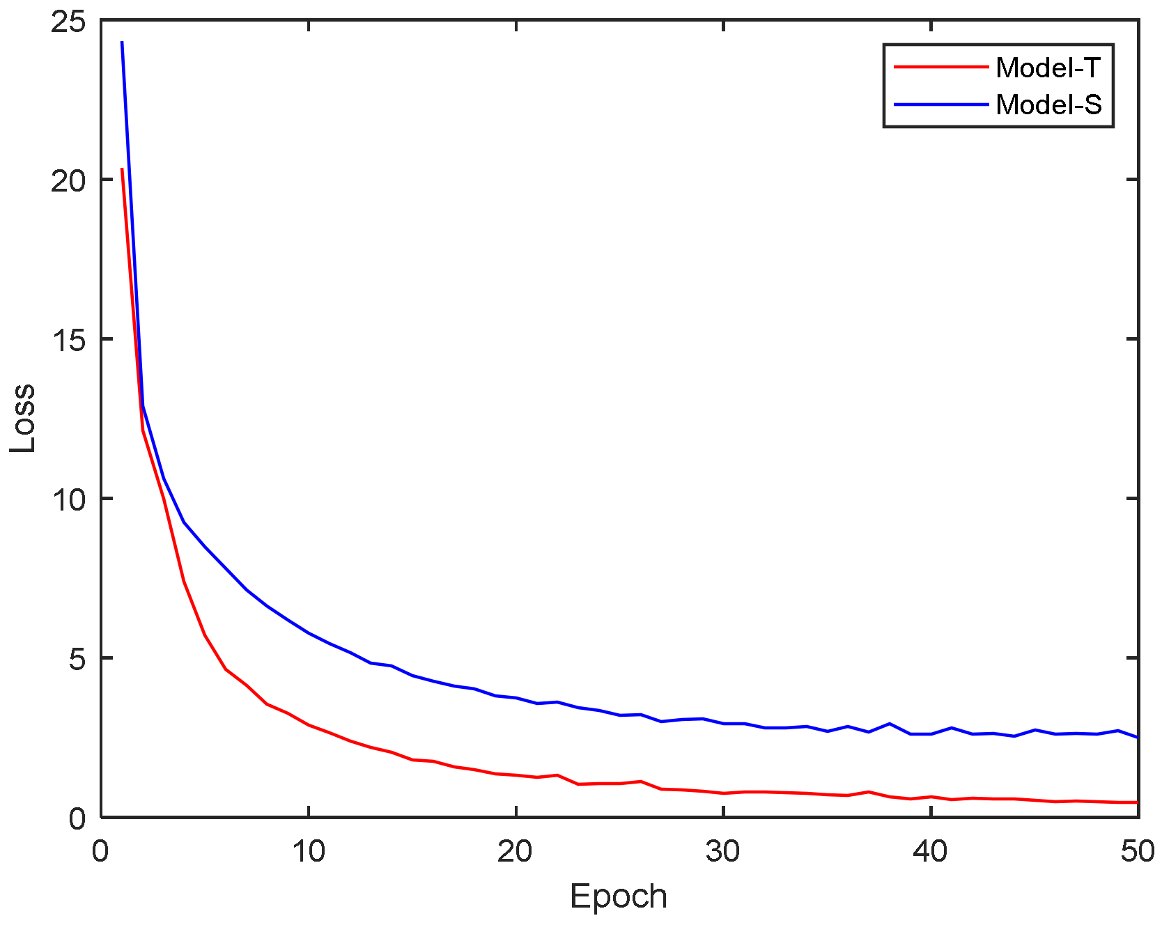
The dataset after the data preprocessing module is subjected to a shuffle operation, i.e., the order of the dataset is randomly disrupted as a way to avoid the phenomenon of the overfitting of the network model caused by the fixed order of the dataset. The training set is partitioned into 70% for model training and 30% for testing. The training accuracy as well as the loss of Model-T and Model-S are shown in
Figure 5 and
Figure 6:
In the process of knowledge distillation, the student model tries to learn the decision basis and feature representation of the teacher model by observing the predictions of the teacher model. As the number of iterations increases, the student model gradually benefits from the knowledge of the teacher model. The parameters of the student model gradually converge to those that can more accurately mimic those of the teacher model and the student model becomes more attuned to the key features of the task and reduces overfitting, thus improving its predictive ability and leading to an increase in recognition accuracy. The simulation results show that the accuracy of both Model-S and Model-T gradually improves with the number of training iterations, i.e., the accuracy of the final converged value of Model-S is 95.84%, and the accuracy of the final converged value of Model-T is 99.07%. The loss of both networks decreases against the increase in the number of iterations, which indicates that the optimization of the model is improving. The reduced loss rate means that the simplified model is more successful in mimicking the predictive distribution of the complex model. By minimizing the loss function, the simplified model gradually learns from the complex model to perform better on similar tasks.
In order to further streamline the parameters of Model-S, it is pruned before the knowledge transfer between Model-S and Model-T, with the goal of reducing the excessive parameter redundancy in Model-S, accelerating the model derivation speed, and making it more suitable to be deployed in service scenarios with high requirements on accuracy and efficiency.
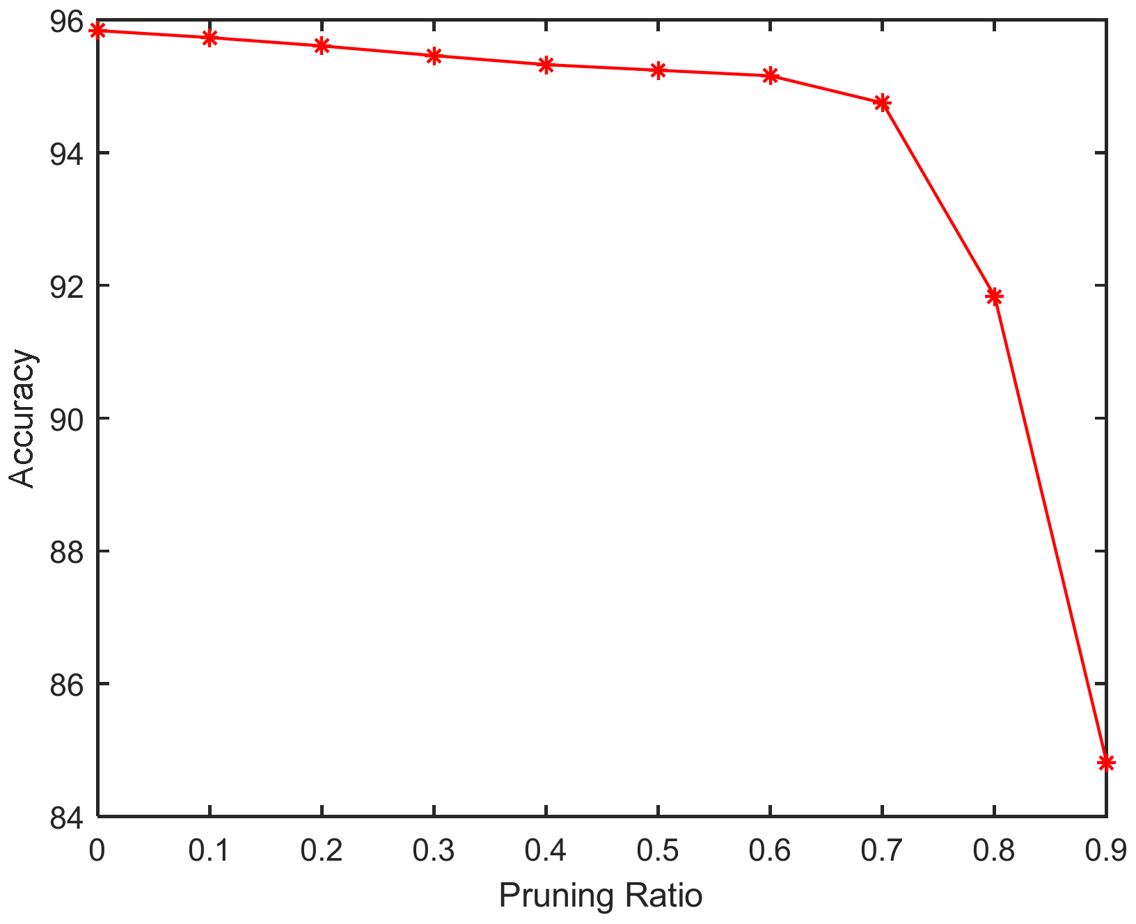
Figure 7 shows the change in Model-S accuracy under different pruning ratios:
Although model pruning can reduce model parameters, the accuracy of the pruned model is often not as good as the original model. The simulation results show that when the pruning ratio is only 0.1, the Model-S recognition accuracy rate increases slightly, indicating that the appropriate amount of pruning can not only accelerate the inference speed of the model but also reduce the network redundancy and improve the network accuracy rate. When the pruning ratio decreases to 0.7, the network accuracy rate decreases less, indicating that the deleted convolutional kernel at this time has less impact on the network accuracy rate; with the pruning ratio increasing again, the network accuracy rate shows a cliff-like decline, indicating that the deleted convolutional kernel at this time has a greater impact on the network accuracy rate. In order to compress the network model as much as possible under the premise of guaranteeing accuracy, this paper chooses a pruning ratio of 0.7 as the student network after pruning to carry out the following accuracy recovery experiments. The accuracy of the model before pruning is 95.84%, and the accuracy of the model after convolution with a ratio of 0.7 is 94.45%. The loss in accuracy of the model before and after pruning is 1.39 percentage points.
Table 5 lists the change in the number of convolution kernels before and after Model-S pruning:
Before engaging in knowledge distillation, the student network needs to go through a network pruning operation to remove the convolutional kernels that have less impact on the final classification result in order to reduce the parameter redundancy of the network and improve the inference speed of the model. From the results, it can be seen that deeper convolutional layers have a higher pruning ratio, this is because the features learned by deeper convolutional layers are more abstract and complex, and therefore have more redundant parameters with a higher pruning ratio.
Figure 8 shows the accuracy comparison of Model-S before and after Model-T guidance after a pruning operation with a pruning ratio of 0.7:
Model-T is the pre-training model, so the model accuracy when Model-T is stabilized is selected for this comparison, which is 99.07%; the temperature coefficient in the knowledge distillation is set to 2, and the cross-loss function between Pruned Model-S and Mode-T accounts for 0.3% of the whole loss function. Model-S before and after distillation both improve the accuracy with the increase of training cycles and it can be seen that the accuracy of the model has stabilized after 30 rounds of epochs. After the 50th round of epochs, the accuracy of Pruned Model-S before distillation improves to 94.45%, and the accuracy of Pruned Model-S after distillation improves to 97.24%, with the latter improved by 2.79 percentage points over the former.
In this paper, all parameters are quantized to four bits, and since knowledge distillation does not change the model structure of the network, the number of parameters of the network does not change, so in the case of fixing the quantization unit, only the number of parameters of the model before and after the pruning needs to be considered.
Table 6 shows the number of parameters of Model-S before and after pruning and the FLOPS transformation.
The results in the above table show that the number of senators and FLOPs of Model-S before and after pruning is drastically reduced, and the number of model senators before pruning is 9.993 × 10⁶, i.e., about 9.99 million. After pruning, the number of modeled senators decreases to 1.804 × 10⁶, i.e., about 1.8 million, and the decrease in the number of modeled senators is 81.9%. This shows that the pruning strategy effectively removes the redundant parameters from the model. The FLOPs of the model before pruning is 3.528 × 10⁹, i.e., about 3.5 billion, and after pruning, the FLOPs of the model decreased to 2.778 × 10⁸, i.e., about 280 million. The decrease in the FLOPs of the model is 92.1% which shows that the pruning strategy is able to reduce the computational complexity of the model. Overall, these data show that the pruning strategy can effectively compress the model, reduce the number of model parameters and computational complexity, and thus improve the efficiency of model training and inference.
In order to compare the recognition efficiency of the proposed algorithm with popular algorithms such as CNN, DPI, and the traditional two-stage service recognition, different numbers of pre-processed completed data were used for testing. All the samples of the traditional two-stage model have to go through the DPI detection module and the deep learning module, while the two-stage model of this paper only inputs the results that DPI fails to recognize into the deep learning model for recognition. The results are shown in
Figure 9.
In this experiment, the data preprocessing time is ignored and only the algorithm prediction time is considered. The simulation results show that with the increase in data volume, the prediction time of all four models shows an upward trend and an approximately linear relationship. The two-stage model has the longest prediction time, the CNN model has the second longest prediction time, and the DPI model has the shortest prediction time. This indicates that the DPI model is more efficient, but the data that cannot be recognized by the DPI model need to be further recognized by the CNN model, which will increase the recognition time. The two-stage approach is more time-consuming compared to a single model, but with a larger amount of data, using the two-stage approach can more effectively utilize the advantages of the DPI model and identify the data that cannot be identified by the DPI through the CNN model, improving the overall recognition accuracy. Compared with the traditional two-stage algorithm, the efficiency of the proposed algorithm in this paper is improved by nearly 18 percentage points. This contributes to the idea that the proposed student network in this paper can obtain an accurate trained model from the teacher network.


