

A Tabu-Matching Heuristic Algorithm Based on Temperature Feasibility for Efficient Synthesis of Heat Exchanger Networks
Abstract
:1. Introduction
2. Model Formulation
2.1. Problem Statements
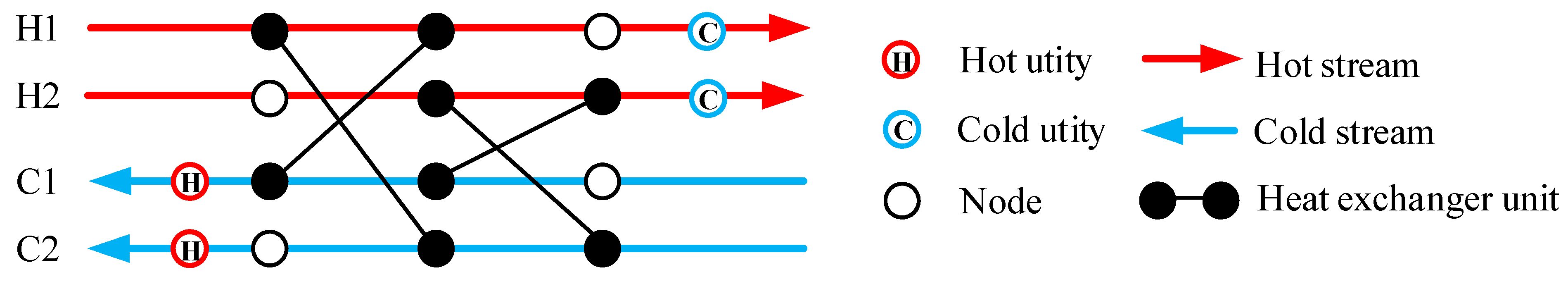
2.2. Non-Structural Model
2.3. Objective Function
2.4. Constraints
- (i)
- Overall heat balance in each stream
- (ii)
- Temperature constraints
3. Solution Approach
3.1. Random Walk Algorithm with Compulsive Evolution
- (1)
- Initialization of individual structure
- (2)
- Random walking operation
- (3)
- Heat exchanger elimination
- (4)
- New heat exchanger unit generation
- (5)
- Selection and mutation operations
- (6)
- Iteration termination
3.2. Infeasible Matching Caused by RWCE
3.2.1. Temperature Crossover
3.2.2. Extreme Match
3.2.3. Adverse Effects of Infeasible Structures
- (1)
- Impact on optimization paths
- (2)
- Impact on optimization efficiency
3.3. RWCE-TB Method
3.3.1. The RWCE-TB Method
3.3.2. Steps of RWCE-TB Method
4. Cases Analysis
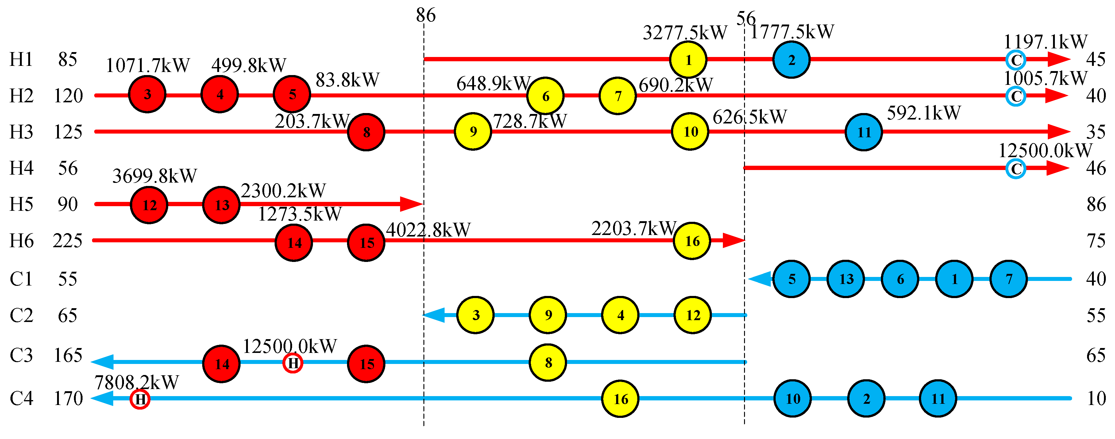
4.1. Case 1 (H6C4)
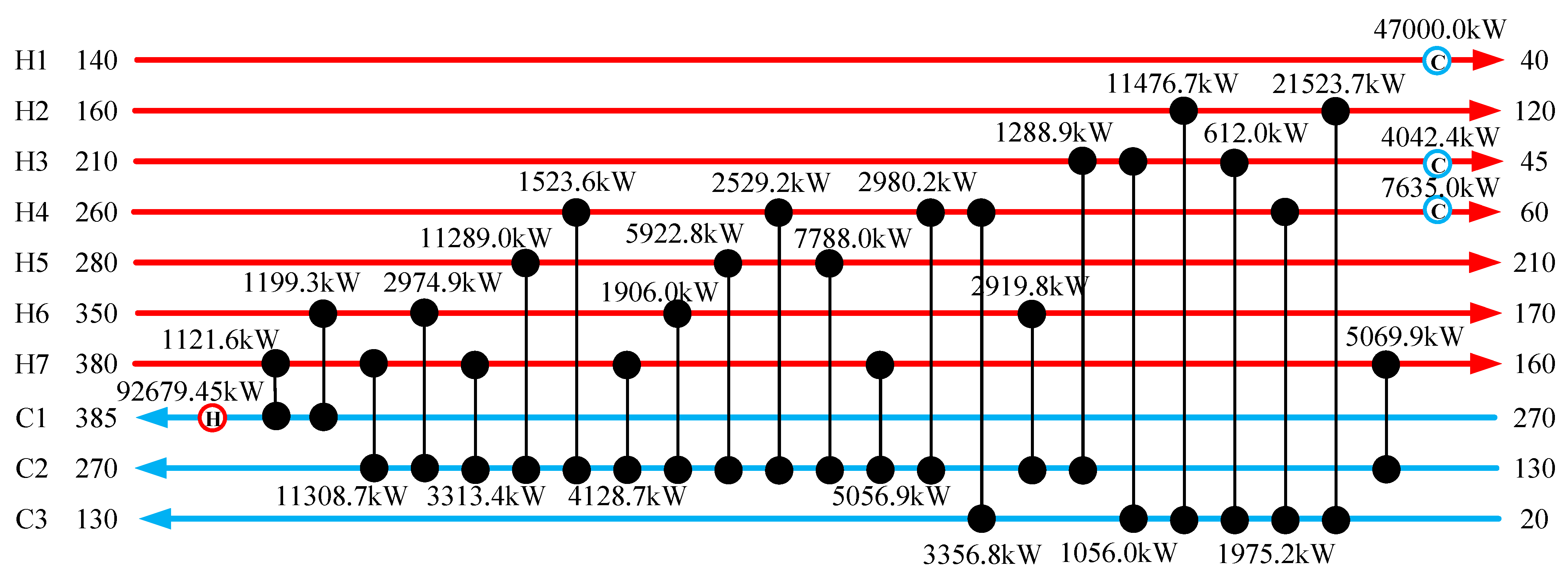
4.2. Case 2 (H7C3)
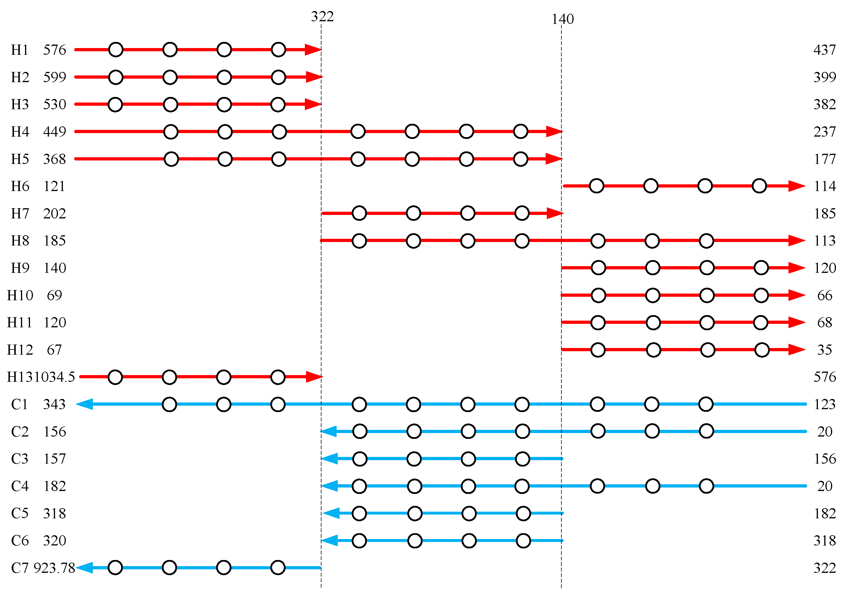
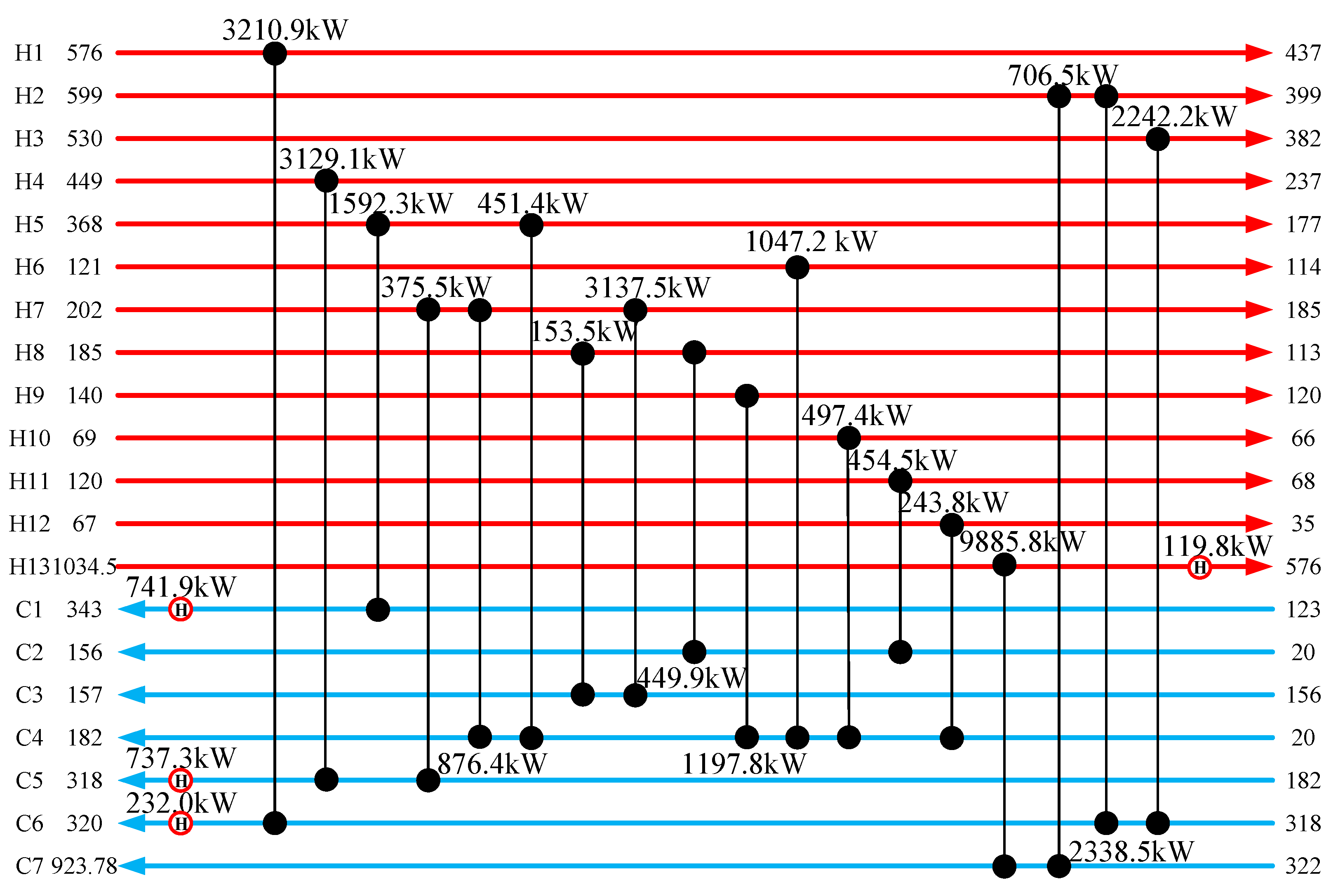
4.3. Case 3 (H13C7)
4.4. Algorithm Efficiency Analysis
5. Conclusions
Author Contributions
Funding
Data Availability Statement
Conflicts of Interest
Nomenclature
| Abbreviations | |
| TAC | Total annual cost |
| HENS | Heat exchanger network synthesis |
| MINLP | Mixed-integer nonlinear programming |
| HEN | Heat exchanger network |
| SWS | Stage-wise superstructure |
| NSM | Non-structural model |
| RWCE | Random walk with compulsive evolution |
| RWCE-TB | Improved Random walk with compulsive evolution with temperature interval tabu matching |
| Variables | |
| A | Heat transfer area, m2 |
| CA | Area cost coefficient of cold utility, heat exchangers, hot utility, USD/yr |
| CCU | Utility cost coefficient of cold utility, USD/yr |
| CHU | Utility cost coefficient of hot utility, USD/yr |
| h | Coefficient of convective heat transfer, kw/m2/°C |
| Q | Heat load, kw |
| QCU | Heat load of cold utility, kW |
| QHU | Heat load of hot utility, kW |
| FFix | Fixed charge of cold utility, heat exchangers, hot utility, USD/yr |
| FCp | Heat capacity flow rate, kw/°C |
| it | Iteration step |
| TAC of individual n at iteration it, USD/yr | |
| ITmax | Maximum number of iterations |
| NP | Population size |
| NH | Number of hot streams |
| NC | Number of cold streams |
| NbH | Number of hot nodes |
| NbC | Number of cold nodes |
| Evolution probability | |
| Qmin | Minimum threshold of heat load, kW |
| Qmax | Maximum threshold of heat load, kW |
| T | Temperature, °C |
| δ | Probability of accepting imperfect solutions |
| △L | The maximum walk step of heat loads, kW |
| ε | Exponent for area cost |
| θ | Generation probability |
| Serial number of the hot stream node | |
| Serial number of the cold stream node | |
| LMTD | Logarithmic mean temperature difference, °C |
| Serial number of the cold node connected with the hot stream node | |
| MH,new | Position of the newly generated hot node |
| MC,new | Position of the newly generated cold node |
| Nmax | The maximum number of nodes of a stream |
| X | Variable is a binary variable with a value range of 0 and 1 |
| ΔTmin | minimum approach temperature, °C |
| NdH | number of node on each hot stream |
| NdC | number of node on each cold stream |
| Superscripts | |
| in | Inlet of streams |
| out | Outlet of streams |
| inner | Inner utility |
| Subscripts | |
| C | Cold stream |
| CU | Cold utility |
| HU | Hot utility |
| H | Hot stream |
| i | Hot stream index |
| j | Cold stream index |
| it | Iteration index |
| min | Minimum |
| inhu | Inner hot utility |
| incu | Inner cold utility |
| new | New heat exchanger unit |
References
- Amer, M.; Chen, M.-R.; Sajjad, U.; Ali, H.M.; Abbas, N.; Lu, M.-C.; Wang, C.-C. Experiments for suitability of plastic heat exchangers for dehumidification applications. Appl. Therm. Eng. 2019, 158, 654–664. [Google Scholar] [CrossRef]
- Short, M.; Isafiade, A.J. Thirty years of mass exchanger network synthesis—A systematic review. J. Clean. Prod. 2021, 304, 127112. [Google Scholar] [CrossRef]
- Chang, C.; Liao, Z.; Bagajewicz, M.J. New superstructure-based model for the globally optimal synthesis of refinery hydrogen networks. J. Clean. Prod. 2021, 292, 126022. [Google Scholar] [CrossRef]
- Kamat, S.; Bandyopadhyay, S.; Foo, D.C.Y.; Liao, Z. State-of-the-art review of heat integrated water allocation network synthesis. Comput. Chem. Eng. 2022, 167, 108003. [Google Scholar] [CrossRef]
- Lin, C.; Wang, B. Combined Heat and Power Dispatch with Start-Stop Schedule of Heat Exchange Stations. In Proceedings of the 2018 IEEE Power & Energy Society General Meeting (PESGM), Portland, OR, USA, 5–9 August 2018; pp. 1–5. [Google Scholar]
- Yang, X.; Sun, Y.; Wu, W.; Liu, H.; Wang, Y. Coordinated real-time power dispatch for integrated transmission and distribution networks based on model-based optimization and deep reinforcement learning. Energy Rep. 2023, 9, 1011–1020. [Google Scholar] [CrossRef]
- Zheng, W.; Lu, H.; Zhang, M.; Wu, Q.; Hou, Y.; Zhu, J. Distributed Energy Management of Multi-Entity Integrated Electricity and Heat Systems: A Review of Architectures, Optimization Algorithms, and Prospects. IEEE Trans. Smart Grid 2023, 1. [Google Scholar] [CrossRef]
- Linnhoff, B.; Flower, J.R. Synthesis of heat exchanger networks: I. Systematic generation of energy optimal networks. AIChE J. 1978, 4, 633–642. [Google Scholar] [CrossRef]
- Linnhoff, B.; Hindmarsh, E. The pinch design method for heat exchanger networks. Chem. Eng. Sci. 1983, 38, 745–763. [Google Scholar] [CrossRef]
- Zamora, J.M.; Grossmann, I.E. A comprehensive global optimization approach for the synthesis of heat exchanger networks with no stream splits. Comput. Chem. Eng. 1997, 21, 65–70. [Google Scholar] [CrossRef]
- Bergamini, M.L.; Grossmann, I.; Scenna, N.; Aguirre, P. An improved piecewise outer-approximation algorithm for the global optimization of MINLP models involving concave and bilinear terms. Comput. Chem. Eng. 2008, 32, 477–493. [Google Scholar] [CrossRef]
- Lin, B.; Miller, D.C. Solving heat exchanger network synthesis problems with Tabu Search. Comput. Chem. Eng. 2004, 28, 1451–1464. [Google Scholar] [CrossRef]
- Dipama, J.; Teyssedou, A.; Sorin, M. Synthesis of heat exchanger networks using genetic algorithms. Appl. Therm. Eng. 2008, 28, 1763–1773. [Google Scholar] [CrossRef]
- Peng, F.; Cui, G. Efficient simultaneous synthesis for heat exchanger network with simulated annealing algorithm. Appl. Therm. Eng. 2015, 78, 136–149. [Google Scholar] [CrossRef]
- Xiao, Y.; Cui, G. A novel Random Walk algorithm with Compulsive Evolution for heat exchanger network synthesis. Appl. Therm. Eng. 2017, 115, 1118–1127. [Google Scholar] [CrossRef]
- Fu, D.; Yu, Z.; Lai, Y. Linking pinch analysis and shifted temperature driving force plot for analysis and retrofit of heat exchanger network. J. Clean. Prod. 2021, 315, 128235. [Google Scholar] [CrossRef]
- Orosz, Á.; How, B.S.; Friedler, F. Multiple-solution heat exchanger network synthesis using P-HENS solver. J. Taiwan Inst. Chem. Eng. 2022, 130, 103859. [Google Scholar] [CrossRef]
- Lakner, R.; Orosz, Á.; How, B.S.; Friedler, F. Synthesis of multiperiod heat exchanger networks: N-best networks with variable approach temperature. Therm. Sci. Eng. Prog. 2023, 42, 137696. [Google Scholar] [CrossRef]
- Yee, T.F.; Grossman, I.E. Simultaneous optimization models for heat integration. II. Heat exchanger network synthesis. Comput. Chem. Eng. 1990, 14, 1165–1184. [Google Scholar] [CrossRef]
- Pavão, L.V.; Costa, C.B.B.; Ravagnani, M.A.S.S. Heat exchanger networks retrofit with an extended superstructure model and a meta-heuristic solution approach. Comput. Chem. Eng. 2019, 125, 380–399. [Google Scholar] [CrossRef]
- Pavão, L.V.; Costa, C.B.B.; Ravagnani, M.A.S.S. A new stage-wise superstructure for heat exchanger network synthesis considering substages, sub-splits and cross flows. Appl. Therm. Eng. 2018, 143, 719–735. [Google Scholar] [CrossRef]
- Na, J.; Jung, J.; Park, C.; Han, C. Simultaneous synthesis of a heat exchanger network with multiple utilities using utility substages. Comput. Chem. Eng. 2015, 79, 70–79. [Google Scholar] [CrossRef]
- Huang, Y.; Zhuang, Y.; Xing, Y.; Liu, L.; Du, J. Multi-objective optimization for work-integrated heat exchange network coupled with interstage multiple utilities. Energy 2023, 273, 127240. [Google Scholar] [CrossRef]
- Xiao, Y.; Kayange, H.A.; Cui, G.; Chen, J. Non-structural model of heat exchanger network: Modeling and optimization. Int. J. Heat Mass Transf. 2019, 140, 752–766. [Google Scholar] [CrossRef]
- Aguitoni, M.C.; Pavão, L.V.; da Silva Sá Ravagnani, M.A. Heat exchanger network synthesis combining Simulated Annealing and Differential Evolution. Energy 2019, 181, 654–664. [Google Scholar] [CrossRef]
- Xiao, Y.; Sun, T.; Cui, G. Enhancing strategy promoted by large step length for the structure optimization of heat exchanger networks. Appl. Therm. Eng. 2020, 173, 115199. [Google Scholar] [CrossRef]
- Xiao, Y.; Cui, G.; Zhang, G.; Ai, L. Parallel optimization route promoted by accepting imperfect solutions for the global optimization of heat exchanger networks. J. Clean. Prod. 2022, 336, 130354. [Google Scholar] [CrossRef]
- Ahmad, S. Heat Exchanger Networks: Cost Tradeoffs in Energy and Capital. Ph.D. Thesis, University of Manchester Institute of Science and Technology (UMIST), Manchester, UK, 1985. [Google Scholar]
- Linnhoff, B.; Ahmad, S.J.C. Engineering, Cost optimum heat exchanger networks—1. Minimum energy and capital using simple models for capital cost. Comput. Chem. Eng. 1990, 14, 729–750. [Google Scholar] [CrossRef]
- Yerramsetty, K.M.; Murty, C.V.S. Synthesis of cost-optimal heat exchanger networks using differential evolution. Comput. Chem. Eng. 2008, 32, 1861–1876. [Google Scholar] [CrossRef]
- Khorasany, R.M.; Fesanghary, M. A novel approach for synthesis of cost-optimal heat exchanger networks. Comput. Chem. Eng. 2009, 33, 1363–1370. [Google Scholar] [CrossRef]
- Zhang, H.; Cui, G.; Xiao, Y.; Chen, J. A novel simultaneous optimization model with efficient stream arrangement for heat exchanger network synthesis. Appl. Therm. Eng. 2017, 110, 1659–1673. [Google Scholar] [CrossRef]
- Rathjens, M.; Fieg, G. A novel hybrid strategy for cost-optimal heat exchanger network synthesis suited for large-scale problems. Appl. Therm. Eng. 2020, 167, 114771. [Google Scholar] [CrossRef]
- Xu, Y.; Cui, G.; Han, X.; Xiao, Y.; Zhang, G. Optimization route arrangement: A new concept to achieve high efficiency and quality in heat exchanger network synthesis. Int. J. Heat Mass Transf. 2021, 178, 121622. [Google Scholar] [CrossRef]
- Chen, J.; Cui, G.; Shen, S. An polymorphic firefly algorithm with self-adaptation strategy for process system heat integration. Case Stud. Therm. Eng. 2023, 47, 103116. [Google Scholar] [CrossRef]
- Ahmad, S.; Patela, E. SUPERTARGET: Applications software for oil refinery retrofit. In Proceedings of the American Institute of Chemical Engineers Spring National Meeting, Houston, TX, USA, 29 March 1987. [Google Scholar]
- Liu, X.W.; Luo, X.; Ma, H.G. Studies on the retrofit of heat exchanger network based on the hybrid genetic algorithm. Appl. Therm. Eng. 2014, 62, 785–790. [Google Scholar] [CrossRef]
- Liu, P.; Cui, G.; Xiao, Y.; Chen, J. A new heuristic algorithm with the step size adjustment strategy for heat exchanger network synthesis. Energy 2018, 143, 12–24. [Google Scholar] [CrossRef]
- Sorsak, A.; Kravanja, Z. MINLP retrofit of heat exchanger networks comprising different exchanger types. In Proceedings of the 12th European Symposium on Computer Aided Process Engineering (ESCAPE-12), The Hague, The Netherlands, 26–29 May 2002; pp. 349–354. [Google Scholar]
- Pavao, L.V.; Costa, C.B.B.; da Silva Sá Ravagnani, M.A. Automated heat exchanger network synthesis by using hybrid natural algorithms and parallel processing. Comput. Chem. Eng. 2016, 94, 370–386. [Google Scholar] [CrossRef]
- Xiao, Y.; Cui, G.; Sun, T.; Chen, J. An integrated random walk algorithm with compulsive evolution and fine-search strategy for heat exchanger network synthesis. Appl. Therm. Eng. 2018, 128, 861–876. [Google Scholar] [CrossRef]
- Zhang, H.; Cui, G. Optimal heat exchanger network synthesis based on improved cuckoo search via Lévy flights. Chem. Eng. Res. Des. 2018, 134, 62–79. [Google Scholar] [CrossRef]
- Xu, Y.; Cui, G.; Deng, W.; Xiao, Y.; Ambonisye, H.K. Relaxation strategy for heat exchanger network synthesis with fixed capital cost. Appl. Therm. Eng. 2019, 152, 184–195. [Google Scholar] [CrossRef]
- Caballero, J.A.; Pavão, L.V.; Costa, C.B.B.; da Silva Sá Ravagnani, M.A. A Novel Sequential Approach for the Design of Heat Exchanger Networks. Front. Chem. Eng. 2021, 3, 733186. [Google Scholar] [CrossRef]
- Chang, C.; Liao, Z.; Costa, A.L.H.; Bagajewicz, M.J. Globally optimal synthesis of heat exchanger networks. Part III: Non-isothermal mixing in minimal and non-minimal networks. AIChE J. 2021, 67, 17393. [Google Scholar] [CrossRef]


| N | ΔL | Qmax | Qmin | τ | θ | δ | Nmax | ITmax | |
|---|---|---|---|---|---|---|---|---|---|
| H6C4 | 10 | 100 | 200 | 5 | 0.2 | 0.2 | 0.01 | 14 | 8 × 10⁸ |
| H7C3 | 30 | 200 | 850 | 5 | 0.2 | 0.2 | 0.005 | 30 | 8 × 10⁸ |
| H13C7 | 30 | 80 | 120 | 10 | 0.2 | 0.2 | 0.01 | 9 | 8 × 10⁸ |
| Stream | Tin (°C) | Tout (°C) | FCp (kW/°C) | h (kW/(m·°C) |
|---|---|---|---|---|
| H1 | 85 | 45 | 156.3 | 0.05 |
| H2 | 120 | 40 | 50.0 | 0.05 |
| H3 | 125 | 35 | 23.9 | 0.05 |
| H4 | 56 | 46 | 1250 | 0.05 |
| H5 | 90 | 86 | 1500 | 0.05 |
| H6 | 225 | 75 | 50 | 0.05 |
| C1 | 40 | 55 | 466.7 | 0.05 |
| C2 | 55 | 65 | 600 | 0.05 |
| C3 | 65 | 165 | 180 | 0.05 |
| C4 | 10 | 170 | 81.3 | 0.05 |
| HU | 200 | 198 | - | 0.05 |
| CU | 15 | 20 | - | 0.05 |
| Annual cost of heat exchanger = 60 A (USD/yr) (A in m2) | ||||
| Annual cost of hot utility = USD 100/kW/yr | ||||
| Annual cost of cold utility = USD 15/kW/yr | ||||
| Literature | Units | Hot Utility/MW | Cold Utility/MW | TAC/USD/yr |
|---|---|---|---|---|
| Ahmad [28] | - | 15,400 | 9796 | 7,074,000 |
| Yerramstetty et al. [30] | 13 | 20,754 | 15,140 | 5,666,756 |
| Khorasany [31] | 12 | 19,605 | 14,000 | 5,662,366 |
| Zhang et al. [32] | 19 | 20,276 | 14,670 | 5,607,762 |
| Peng and Cui [14] | 18 | 20,339 | 14,733 | 5,596,079 |
| Rathjens et al. [33] | 12 | 20,420 | 14,815 | 5,713,267 |
| Xu et al. [34] | 13 | 20,377 | 14,795 | 5,704,465 (with splits) |
| Chen [35] | 19 | 20,540 | 14,935 | 5,592,255 |
| NSM&RWCE (Figure 9) | 22 | 20,250 | 14,644 | 5,589,808 |
| NSM&RWCE-TB (Figure 10) | 21 | 20,308 | 14,703 | 5,588,154 |
| Stream | Tin (°C) | Tout (°C) | FCp (kW/°C) | h (kW/(m2·°C) |
|---|---|---|---|---|
| H1 | 140.0 | 40.0 | 470.0 | 0.8 |
| H2 | 160.0 | 120.0 | 825.0 | 0.8 |
| H3 | 210.0 | 45.0 | 42.4 | 0.8 |
| H4 | 260.0 | 60.0 | 100.0 | 0.8 |
| H5 | 280.0 | 210.0 | 357.1 | 0.8 |
| H6 | 350.0 | 170.0 | 50.0 | 0.8 |
| H7 | 380.0 | 160.0 | 136.4 | 0.8 |
| C1 | 270.0 | 385.0 | 826.1 | 0.8 |
| C2 | 130.0 | 270.0 | 500.0 | 0.8 |
| C3 | 20.0 | 130.0 | 363.6 | 0.8 |
| HU | 500 | 499 | - | 0.8 |
| CU | 20 | 40 | - | 0.8 |
| Annual cost of heat exchanger = 300 A (USD/yr) (A in m2) | ||||
| Annual cost of hot utility = USD 60/kW/yr | ||||
| Annual cost of cold utility = USD 5/kW/yr | ||||
| Literature | Units | Hot Utility/MW | Cold Utility/MW | TAC/USD/yr |
|---|---|---|---|---|
| Ahmad [36] | 11 | - | - | 9,490,000 |
| Liu et al. [37] | 15 | 92.93 | 58.93 | 8,917,245 |
| Liu et al. [38] | 31 | 92.40 | 58.40 | 8,707,983 |
| NSM & RWCE (Figure 12) | 27 | 92.68 | 58.68 | 8,715,491 |
| NSM & RWCE-TB (Figure 13) | 33 | 92.42 | 58.42 | 8,706,548 |
| Stream | Tin (°C) | Tout (°C) | FCp (kW/°C) | h (kW/(m2·°C) |
|---|---|---|---|---|
| H1 | 576 | 437 | 23.1 | 0.06 |
| H2 | 599 | 399 | 15.22 | 0.06 |
| H3 | 530 | 382 | 15.15 | 0.06 |
| H4 | 449 | 237 | 14.76 | 0.06 |
| H5 | 368 | 177 | 10.7 | 0.06 |
| H6 | 121 | 114 | 149.6 | 1.0 |
| H7 | 202 | 185 | 258.2 | 1.0 |
| H8 | 185 | 113 | 8.38 | 1.0 |
| H9 | 140 | 120 | 59.89 | 1.0 |
| H10 | 69 | 66 | 165.79 | 1.0 |
| H11 | 120 | 68 | 8.74 | 1.0 |
| H12 | 67 | 35 | 7.62 | 1.0 |
| H13 | 1034.5 | 576 | 21.3 | 0.06 |
| C1 | 123 | 343 | 10.61 | 0.06 |
| C2 | 20 | 156 | 6.65 | 1.2 |
| C3 | 156 | 157 | 3291 | 2.0 |
| C4 | 20 | 182 | 26.63 | 1.2 |
| C5 | 182 | 318 | 31.19 | 1.2 |
| C6 | 318 | 320 | 4011.83 | 2.0 |
| C7 | 322 | 923.78 | 17.6 | 0.06 |
| HU | 927 | 927 | - | 5.0 |
| CU | 9 | 17 | - | 1.0 |
| Annual cost of heat exchanger = 4000 + 500 A0.83 (USD/yr) (A in m2) | ||||
| Annual cost of hot utility = USD 250/kW/yr | ||||
| Annual cost of cold utility = USD 25/kW/yr | ||||
| Literature | Units | Hot Utility/MW | Cold Utility/MW | TAC/USD/yr |
|---|---|---|---|---|
| Pavão et al. [40] | 21 | 1938 | 106.93 | 1,516,482 (with splits) |
| Xiao et al. [41] | 23 | 1.868 | 36.6 | 1,447,482 |
| Zhang et al. [42] | 22 | 1.831 | 0.00 | 1,418,981 |
| Xu et al. [43] | 21 | 1.831 | 0.04 | 1,412,801 |
| Caballero et al. [44] | 21 | 1.831 | 0.00 | 1,414,831(with splits) |
| Chang [45] | 20 | 1.831 | 0.00 | 1,407,203 (with splits) |
| NSM & RWCE (Figure 15) | 22 | 1.831 | 0.00 | 1,401,311 |
| NSM & RWCE-TB (Figure 16) | 21 | 1.831 | 0.00 | 1,395,971 |
| Case | Computational Time (s) of the NSM & RWCE | Computational Time (s) of the NSM & RWCE-TB | Efficiency Improvement (%) |
|---|---|---|---|
| case1 | 10,585 | 8891 | 16.0% |
| case2 | 13,311 | 9158 | 31.2% |
| case3 | 64,619 | 50,209 | 22.3% |
Disclaimer/Publisher’s Note: The statements, opinions and data contained in all publications are solely those of the individual author(s) and contributor(s) and not of MDPI and/or the editor(s). MDPI and/or the editor(s) disclaim responsibility for any injury to people or property resulting from any ideas, methods, instructions or products referred to in the content. |
© 2023 by the authors. Licensee MDPI, Basel, Switzerland. This article is an open access article distributed under the terms and conditions of the Creative Commons Attribution (CC BY) license (https://creativecommons.org/licenses/by/4.0/).
Share and Cite
Huang, X.; Shen, H.; Yue, W.; Duan, H.; Cui, G. A Tabu-Matching Heuristic Algorithm Based on Temperature Feasibility for Efficient Synthesis of Heat Exchanger Networks. Processes 2023, 11, 2713. https://doi.org/10.3390/pr11092713
Huang X, Shen H, Yue W, Duan H, Cui G. A Tabu-Matching Heuristic Algorithm Based on Temperature Feasibility for Efficient Synthesis of Heat Exchanger Networks. Processes. 2023; 11(9):2713. https://doi.org/10.3390/pr11092713
Chicago/Turabian StyleHuang, Xiaohuang, Hao Shen, Wenhao Yue, Huanhuan Duan, and Guomin Cui. 2023. "A Tabu-Matching Heuristic Algorithm Based on Temperature Feasibility for Efficient Synthesis of Heat Exchanger Networks" Processes 11, no. 9: 2713. https://doi.org/10.3390/pr11092713