Economic Dispatch of AC/DC Power System Considering Thermal Dynamics

Abstract

Advance in renewable penetration has promoted the interaction between the AC and DC power system and multi-energy sources. However, the disparate nature of different energy utilization technologies presents strong challenges for the economic dispatch of such a complex system. This paper proposes a comprehensive characterization of the AC/DC power system considering multi-energy and renewable integration. Detailed models are elaborated for the AC/DC power grid, the district heating system (DHS), coupling units, and renewables to describe their inner interactions accurately. On this basis, an economic dispatch method is developed to minimize the operation cost and renewable’s abandonment. Simulations indicate that the interaction between the AC/DC power systems and multi-energy sources can enhance voltage levels and improve operational economy.

1. Introduction

In recent years, the escalating conflict between increasing energy consumption and the pressing environmental crisis has expedited the transition from conventional coal-based power systems to renewable energy-based power systems [1,2,3]. In order to facilitate and advance this shift, various technologies have emerged to enhance the integration of renewables, including the interaction between AC and DC power systems [4,5], as well as multi-energy integration [6,7], among others. Among these technologies, the interaction between AC and DC grids stands out due to its remarkable flexibility and adjustability, and, as a result, it has garnered significant attention as a prominent research area in recent years.

In this context, large amounts of research have been conducted to investigate operational analysis in the AC/DC power system. The majority can be classified into two types, i.e., from the solution perspective and the scenario perspective. From the solution aspect, reference [8] proposed a unified approach to formulate the power flow model in AC/DC hybrid microgrids, where an extended Newton method was developed to solve the nonlinear model. Although the Newton-based method is the most accurate, massive nonlinear terms in the corresponding optimization model make it an NP-hard problem, which is difficult to solve. To address the strong nonlinearity, reference [9] further proposed a second-order cone programming method for optimization in the AC/DC power system. Similarly, reference [10] presented a semidefinite relaxation method for the optimal power flow in the AC/DC power system. Although these relaxation-based methods improve the solution efficiency with some nonlinear terms reserved, it is challenging to guarantee the uniqueness of the optimized results [11]. Therefore, different from the mentioned works that directly solve the nonlinear AC/DC power flow model, reference [12] proposed an improved DC power flow model that incorporates voltage magnitude considerations to address the optimization problem in the AC/DC grid. By preserving nonlinearity, this method adopts iterative optimization techniques to obtain a unique solution, which is widely adopted in current research studies.

From the scenario perspective, reference [13] explored the optimal power flow problem in a transmission–distribution AC/DC power system, taking into account multi-source complementarity and demand response. Building upon this, reference [14] analyzed the uncertainties associated with renewables and load distribution in the AC/DC power system, and developed a robust optimization method for economic dispatch. Additionally, reference [15] examined the coordination of active–reactive power in the AC/DC power system, comparing two control strategies to minimize the actions of reactive devices. A detailed model of the voltage source converter (VSC) was also introduced in [16], proposing a novel linear VSC model that simplifies the day-ahead scheduling problem and enhances the solvability of the optimization model using Taylor expansion. Considering the impact of frequent adjustments on the service life of reactive devices, reference [17] treated the actions of reactive devices as constraints, constructing a two-stage day-ahead stochastic scheduling model for the AC/DC power system. However, this work formulated the problem as a mixed-integer nonlinear programming (MINLP) problem. Diverging from the aforementioned studies, reference [18] introduced electricity–gas coupling into the AC/DC power system for optimal scheduling, incorporating the influence of market environments to enrich the optimization problem. As the problem was nonlinear, the second-order cone programming method was employed to transform it into a mixed-integer linear programming problem (MILP) for improved solvability. In [19], the scheduling problem considered the detailed model of the electricity–gas coupling unit, specifically the gas turbine. The research further highlighted the significant influence of multi-energy integration on reactive power optimization and how it can promote wind power penetration.

In summary, despite significant efforts devoted to investigating the operation of AC/DC power systems, several gaps still remain as follows.

(1)

Existing studies mainly focus on renewables such as wind turbines (WTs) and photovoltaics (PVs) as simple active power generators, neglecting their reactive power output and its corresponding impact on power system operation.

(2)

Most studies concentrate on modeling a single component and apply it to operational analyses of the power system, such as AC/DC power system interaction, active–reactive power coordinate optimization, and electricity–gas coupling. However, a comprehensive investigation of economic dispatch in the AC/DC power system considering multi-energy integration and renewable penetration is lacking. Moreover, the current studies mainly focus on the active power coordination in the AC/DC power system dispatch, while the reactive power output of the renewables is neglected. Thus, the full potential of the modern power system to promote renewable consumption is unexplored.

(3)

Regarding the model of multi-energy integration, numerical methods like the finite difference method (FDM) and the node method (NM) are commonly used to discretize dynamic energy flow equations. However, this introduces numerous discrete variables, hindering the efficient solution of optimization problems.

To overcome the deficiencies, this paper first derives the modeling of the AC/DC power system with the district heating system (DHS) and renewable integration in detail. On this basis, an economic dispatch method is proposed to investigate the active–reactive power and thermal power coordination in the AC/DC power system. The main contributions of this paper are summarized below.

(1)

We have meticulously developed a comprehensive model for the AC/DC power system considering the integration of multi-energy and renewables. Within this model, the AC/DC power system is described using an improved DC power flow formulation. Meanwhile, the multi-energy system, specifically the DHS, is characterized by a fully analytical model (FAM). This choice eliminates the need for numerical discretization, substantially enhancing both modeling accuracy and efficiency.

(2)

We have proposed a novel economic dispatch method, which enables the coordinated operation of active, reactive, and thermal power components alongside the renewable energy sources within the AC/DC power system. This method functionality not only promotes the effective utilization of renewables but also contributes to cost reduction efforts.

The remainder of this paper is as follows. The model of the AC/DC power system considering DHS and renewable integration is presented in Section 2. The economic dispatch method is developed in Section 3. The case study and conclusion are given in Section 4 and Section 5, respectively.

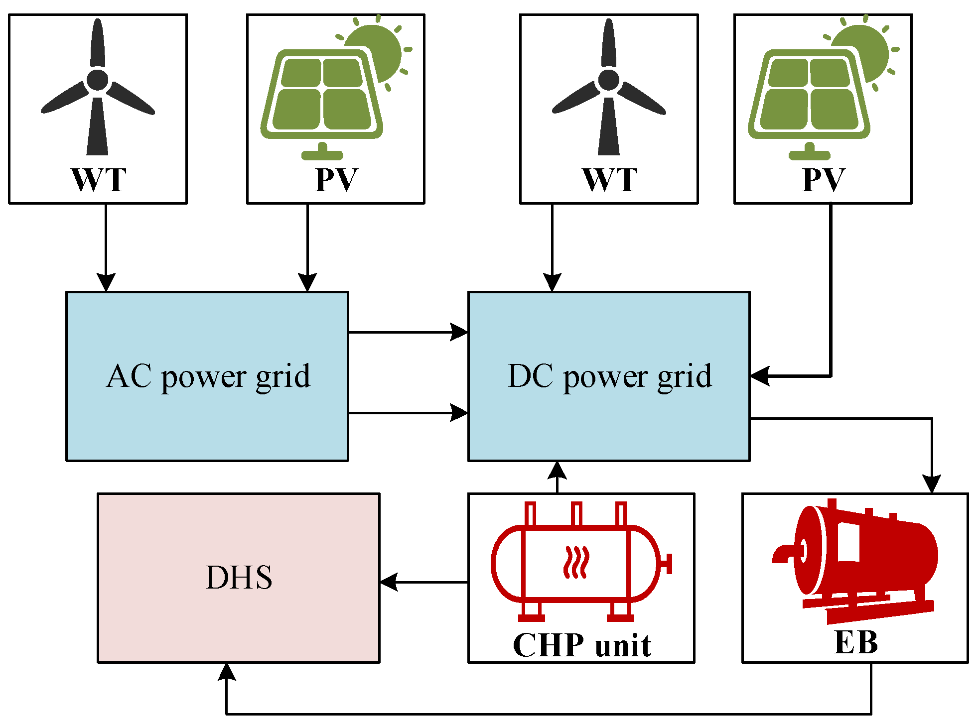
2. Model of AC/DC Power System Considering Thermal Dynamics

Figure 1 illustrates the schematic of the AC/DC power system with the DHS and renewable integration. As shown in the figure, the system consists of three subsystems: the AC power system, the DC power system, and the DHS. WTs and PVs are integrated into both the AC and DC power systems. The DHS is connected to the DC power system through the combined heat and power (CHP) unit and the electric boiler (EB). This allows for bidirectional transfer of electric and thermal power between the power system and the DHS. Hence, this section primarily focuses on the comprehensive modeling of the AC/DC power system, the DHS, and the coupling units.

2.1. AC/DC Power System

The power system model serves as the fundamental framework for economic dispatch by employing the AC power flow equations. These equations effectively depict the power flow balance at the electric buses and branches [11], as illustrated below.

$$\begin{array}{l}{P}_{WT,i}+P_{PV,i}+P_{G,i}-P_{L,i}=\\ \hspace{1em}\hspace{1em}{U}_i{\displaystyle \sum _j{U}_j(G_{ij}\cos {\theta }_{ij}+B_{ij}\sin {\theta }_{ij})}\hspace{1em}i,j\in {\mathsf{\Theta }}_{AC}^e\end{array}$$

(1)

$$\begin{array}{l}{Q}_{WT,i}+Q_{PV,i}+Q_{G,i}-Q_{L,i}=\\ \hspace{1em}\hspace{1em}\hspace{1em}\hspace{1em}\hspace{1em}\hspace{1em}{U}_i{\displaystyle \sum _j{U}_j(G_{ij}\sin {\theta }_{ij}-B_{ij}\cos {\theta }_{ij})}\hspace{1em}i,j\in {\mathsf{\Theta }}_{AC}^e\end{array}$$

(2)

$$P_{l,ij}=U_i{U}_j(G_{ij}\cos {\theta }_{ij}+B_{ij}\sin {\theta }_{ij})-G_{ij}{U}_i^2\hspace{1em}i,j\in {\mathsf{\Theta }}_{AC}^e$$

(3)

$$Q_{l,ij}=U_i{U}_j(G_{ij}\sin {\theta }_{ij}-B_{ij}\cos {\theta }_{ij})+B_{ij}{U}_i^2\hspace{1em}i,j\in {\mathsf{\Theta }}_{AC}^e$$

(4)

In the AC power system, ${\mathsf{\Theta }}_{AC}^e$ represents the set of buses; P_G and Q_G denote the active and reactive power generation, respectively; P_L and Q_L represent the active and reactive power consumption, respectively; U and θ refer to the voltage magnitude and phase angle, respectively; G_ij and B_ij correspond to the real and imaginary components of the admittance between buses i and j, respectively; P_WT and Q_WT represent the active and reactive output of the WT, respectively; and P_PV and Q_PV represent the active and reactive output of the PV, respectively.

By expanding sinθ_ij and cosθ_ij using Taylor series and retaining the linear and quadratic terms, the following formula can be derived for the AC power system [12].

$$\sin {\theta }_{ij}\approx {\theta }_{ij}, \cos {\theta }_{ij}\approx 1-\frac{{\theta }_{ij}^2}{2}\hspace{1em}i,j\in {\mathsf{\Theta }}_{AC}^e$$

(5)

Taking into account that the voltage magnitudes of electric buses are approximately 1.0 p.u., the following formulas can be simplified:

$$U_i{U}_j{\theta }_{ij}\approx {\theta }_{ij},\hspace{1em}{U}_i{U}_j{\theta }_{ij}^2\approx {\theta }_{ij}^2\hspace{1em}i,j\in {\mathsf{\Theta }}_{AC}^e$$

(6)

By substituting Equations (5) and (6) into Equations (3) and (4), the branch power flow equations are reformulated as [12]:

$$P_{l,ij}=G_{ij}\frac{U_i^2-U_j^2}{2}-B_{ij}{\theta }_{ij}+P_{l,ij}^{loss}\hspace{1em}i,j\in {\mathsf{\Theta }}_{AC}^e$$

(7)

$$Q_{l,ij}=-B_{ij}\frac{U_i^2-U_j^2}{2}-G_{ij}{\theta }_{ij}+Q_{l,ij}^{loss}\hspace{1em}i,j\in {\mathsf{\Theta }}_{AC}^e$$

(8)

$$P_{l,ij}^{loss}=G_{ij}\frac{{\theta }_{ij}^2+U_{ij}^2}{2},Q_{l,ij}^{loss}=B_{ij}\frac{{\theta }_{ij}^2+U_{ij}^2}{2}\hspace{1em}i,j\in {\mathsf{\Theta }}_{AC}^e$$

(9)

where $P_{l,ij}^{loss}$ and $Q_{l,ij}^{loss}$ are the active and reactive branch power loss between buses i and j, respectively.

By substituting Equations (7)–(9) into Equations (1) and (2), the power balance at the electric buses can be expressed as:

$$P_{WT,i}+P_{PV,i}+P_{G,i}-P_{L,i}={\displaystyle \sum _{i,j}{P}_{l,ij}}+{\displaystyle \sum _{i,j}{G}_{ij}{U}_i^2}\hspace{1em}i,j\in {\mathsf{\Theta }}_{AC}^e$$

(10)

$$Q_{WT,i}+Q_{PV,i}+Q_{G,i}-Q_{L,i}={\displaystyle \sum _{i,j}{Q}_{l,ij}}-{\displaystyle \sum _{i,j}{B}_{ij}{U}_i^2}\hspace{1em}i,j\in {\mathsf{\Theta }}_{AC}^e$$

(11)

The model of the DC power system follows a similar structure to that of the AC power system, with the distinction that phase angles and reactive power terms are disregarded [10,12,19]. Based on Equations (7)–(11), the branch power flow equation for the DC power system is expressed as:

$$P_{l,ij}=G_{ij}\frac{U_i^2-U_j^2}{2}+G_{ij}\frac{U_{ij}^2}{2}\hspace{1em}i,j\in {\mathsf{\Theta }}_{DC}^e$$

(12)

2.2. Heating System

The DHS comprises two symmetric networks, namely the supply network and the return network. In the DHS, the heating source initially generates thermal power to heat the water. Subsequently, the high-temperature water is conveyed through the supply pipelines and utilized by the heating loads. After transferring the thermal power, the high-temperature water in the supply network cools down and circulates back into the return network, returning from the heating loads to the heating sources. Consequently, the variable distribution within the DHS is jointly determined by the hydraulic and thermal states [20].

This paper focuses on the DHS operating in quality regulation mode, wherein the supply temperature is continuously adjusted to meet consumer demands while the mass flow rates remain fixed. This mode is widely adopted in various regions such as China, Northern Europe, and Russia due to its simpler operation and more stable hydraulic states [21,22]. In this context, our primary focus is directed towards the thermal aspects of the DHS model, as depicted in the following equations.

$${\varphi }_i=C_w{m}_i\left(T_{i,t}^s-T_{i,t}^s\right)\hspace{1em}i\in {\mathsf{\Theta }}^h\cup {\mathsf{\Phi }}^h$$

(13)

$$\frac{\partial T_i^s}{\partial t}+v_i\frac{\partial T_i^s}{\partial x}+\frac{v_i}{C_w{m}_i{\lambda }_i}{T}_i^s=0\hspace{1em}i\in {\mathsf{\Phi }}^h$$

(14)

$$\frac{\partial T_i^r}{\partial t}+v_i\frac{\partial T_i^r}{\partial x}+\frac{v_i}{C_w{m}_i{\lambda }_i}{T}_i^r=0\hspace{1em}i\in {\mathsf{\Phi }}^h$$

(15)

$$T_i^s{\displaystyle \sum _{b\in {\mathsf{\Phi }}_{s,i}^h}{m}_b={\displaystyle \sum _{k\in {\mathsf{\Phi }}_{e,i}^h}{m}_k{T}_{k,\mathrm{o}}^s}}\hspace{1em}i\in {\mathsf{\Theta }}^h$$

(16)

$$T_i^r{\displaystyle \sum _{b\in {\mathsf{\Phi }}_{s,i}^h}{m}_b={\displaystyle \sum _{k\in {\mathsf{\Phi }}_{e,i}^h}{m}_k{T}_{k,\mathrm{o}}^r}}\hspace{1em}i\in {\mathsf{\Theta }}^h$$

(17)

$$T_{b,\mathrm{i}}^s=T_k^s\hspace{1em}b\in {\mathsf{\Phi }}_{s,k}^h,k\in {\mathsf{\Theta }}^h$$

(18)

$$T_{b,\mathrm{i}}^r=T_k^r\hspace{1em}b\in {\mathsf{\Phi }}_{s,k}^h,k\in {\mathsf{\Theta }}^h$$

(19)

In the mentioned equations, Θ^h and Φ^h represent the sets of the nodes and pipes in the DHS, respectively; ϕ represents the thermal power; C_w represents the specific heat capacity of the hot water; λ represents the pipe thermal resistance in the DHS; and m represents the mass flow rate. Furthermore, ${\mathsf{\Phi }}_{s,i}^h$ represents the set of pipes leaving from node i; ${\mathsf{\Phi }}_{e,i}^h$ represents the set of pipes ending at node i; $T_i^s$ and $T_i^r$ represent the supply and return temperature of node i, respectively; and $T_{b,\mathrm{i}}^s$ and $T_{b,\mathrm{i}}^r$ represent the inlet temperature of pipe b in the supply and return networks, respectively. Similarly, $T_{b,\mathrm{o}}^s$ and $T_{b,\mathrm{o}}^r$ represent the outlet temperature of pipe b in the supply and return networks, respectively.

In the given equations, Equation (13) represents the node model in the DHS. Equations (14), (16) and (18) correspond to the thermal model in the supply network. On the other hand, Equations (15), (17) and (19) represent the thermal model in the return network. Specifically, Equations (14) and (15) describe the temperature distribution along the pipe, representing the pipe temperature transportation equations; Equations (16) and (17) depict the energy conservation at the nodes, serving as the node temperature mixture equations. Lastly, Equations (18) and (19) are topological equations that ensure consistency between the node and pipe temperatures.

2.3. Coupling Unit

In this paper, the coupling between the DHS and the DC power system involves the widely used extraction CHP unit and the EB. The extraction CHP unit cogenerates the electric and thermal power. The feasible region is employed to characterize the range of output thermal power and electric power output of the CHP unit, as presented below [20].

$$\left\{\begin{array}{l}0\le P_{chp}\le P_{chp,\max }^{},\\ 0\le {\varphi }_{chp}\le {\varphi }_{chp,\max }^{}\\ {\alpha }_{chp1}{\varphi }_{chp}\le P_{chp}\le P_{chp,\max }-{\alpha }_{chp2}{\varphi }_{chp}\end{array}\right.$$

(20)

In Equation (20), P_chp and ϕ_chp denote the electric power output and thermal power output of the CHP unit, respectively; P_chp,max and ϕ_chp,max represent the electric power and thermal power capacities of the CHP unit, respectively; and α_chp1 and α_chp2 represent the electric–thermal ratios of the CHP unit, respectively. The EB consumes electric power to generate thermal power and their relationship is described by efficiency, as illustrated below.

$${\varphi }_{eb}={\alpha }_{eb}{P}_{eb}$$

(21)

where P_eb represents the consumed electric power of the EB and ϕ_eb represents the output thermal power of the EB.

3. Economic Dispatch Method of AC/DC Power System

Building upon the models introduced in Section 2, this section introduces the economic dispatch method for the AC/DC power system incorporating the DHS and renewable energy integration.

3.1. Objective Function

The objective function of this paper is twofold: to minimize operating costs and maximize renewable energy consumption. Hence, the objective function can be formulated as follows:

$$C=\min {\displaystyle \sum _{t\in \mathrm{\Gamma }}\left(C_{P,t}+C_{\varphi ,t}+C_{WT,t}+C_{PV,t}\right)}$$

(22)

where Γ represents the time label to be optimized, i.e., Γ = {1, 2, 3, …., 24}; C_P represents the operating costs in the AC/DC power system; C_ϕ represents the operating costs in the DHS; C_WT represents the operating costs of the WT, encompassing maintenance costs and penalties for abandonment; and C_PV represents the operating costs of the PV, including the maintenance cost and the penalty cost for abandonment.

To elaborate, the operating cost of the electric power generation in the AC/DC power system can be expressed as follows [15]:

$$C_{P,t}{\displaystyle \sum _{i\in {\mathsf{\Theta }}_G^e\cup {\mathsf{\Theta }}_{DC}^e}\left({\beta }_{1,i}{P}_{G,i,t}^2+{\beta }_{2,i}{P}_{G,i,t}+{\beta }_{3,i}\right)}$$

(23)

where ${\mathsf{\Theta }}_G^e$ represents the set of generator buses in the AC/DC power system, including the traditional generators and the extraction CHP units; β₁–β₃ are the cost coefficients of the electric power generation.

The operating cost of the thermal power generation in the DHS is expressed as:

$$C_{\varphi ,t}={\displaystyle \sum _{i\in {\mathsf{\Theta }}^{chp}}\left({\eta }_{1,i}{\varphi }_{chp,i,t}^2+{\eta }_{2,i}{\varphi }_{chp,i,t}+{\eta }_{3,i}\right)}$$

(24)

where Θ^chp represents the set of CHP units and η₁-η₃ are the constant coefficients of the CHP units’ cost for heating purposes.

The operating costs of the WT and PV are expressed as:

$$C_{WT,t}={\displaystyle \sum _{i\in {\mathsf{\Theta }}^{WT}}\left({\alpha }_{WT,i}{P}_{WT,i,t}+{\mu }_{WT}\left(P_{WT,i,t,\max }-P_{WT,i,t}\right)\right)}$$

(25)

$$C_{PV,t}={\displaystyle \sum _{i\in {\mathsf{\Theta }}^{PV}}\left({\alpha }_{PV,i}{P}_{PV,i,t}+{\mu }_{PV}\left(P_{PV,i,t,\max }-P_{PV,i,t}\right)\right)}$$

(26)

where Θ^PV and Θ^WT represent the sets of the buses connected with PVs and WTs, respectively; α_PV and α_WT represent the unit cost for the maintenance of the PVs and WTs, respectively; P_PV,i,t,max and P_WT,i,t,max represent the maximum active power output of the ith PV and WT at t, respectively; and μ_PV and μ_WT represent the unit penalty for the abandonment of the PVs and WTs, respectively.

3.2. Constraints from Power System Side

The constraints in the AC/DC power system contain the security constraints and the capacity constraints of the bidirectional converter between the AC power system and the DC power system. Their detailed expressions are provided below.

$$\left\{\begin{array}{l}{U}_{i,\min }^{}\le U_i\le U_{i,\max }^{}\\ U_{j,\min }^{}\le U_j\le U_{j,\max }^{}\end{array}\right.\hspace{1em}i\in {\mathsf{\Theta }}_{AC}^e,j\in {\mathsf{\Theta }}_{DC}^e$$

(27)

$$-\frac{\pi }{2}\le {\theta }_i\le \frac{\pi }{2}\hspace{1em}i\in {\mathsf{\Theta }}_{AC}^e$$

(28)

$$\left\{\begin{array}{l}{P}_{l,ij}^2+Q_{l,ij}^2\le S_{l,ij,\max }^2\hspace{1em}\hspace{1em}\hspace{1em}\hspace{1em}i,j\in {\mathsf{\Theta }}_{AC}^e\\ -P_{l,mn,\max }^{}\le P_{l,mn}^{}\le P_{l,mn,\max }^{}\hspace{1em}m,n\in {\mathsf{\Theta }}_{DC}^e\end{array}\right.$$

(29)

$$\left\{\begin{array}{l}{P}_{G,i,\min }\le P_{G,i}\le P_{G,i,\max }\hspace{1em}i\in {\mathsf{\Theta }}_{AC}^e\\ P_{G,j,\min }\le P_{G,j}\le P_{G,j,\max }\hspace{1em}j\in {\mathsf{\Theta }}_{DC}^e\end{array}\right.$$

(30)

$$Q_{G,i,\min }\le Q_{G,i}\le Q_{G,i,\max }\hspace{1em}i\in {\mathsf{\Theta }}_{AC}^e$$

(31)

$$-P_{l,ij,\max }\le P_{l,ij}\le P_{l,ij,\max }\hspace{1em}i\in {\mathsf{\Theta }}_{AC}^e,j\in {\mathsf{\Theta }}_{DC}^e$$

(32)

where U_min and U_max represent the minimum and maximum limits of the voltage magnitude, respectively; S_l,ij,max represents the maximum apparent branch power flow between buses i and j; P_G,min and P_G,max represent the minimum and maximum limits of the active power output of the generator, respectively; Q_G,min and Q_G,max represent the minimum and maximum limits of the reactive power output of the generator, respectively; and P_l,ij,max represents the maximum interactive active power between the AC power system and the DC power system.

In the above equations, Equations (27) and (28) represent the voltage magnitude and phase angle constraints, respectively; Equation (29) represents the branch power flow constraint; Equations (30) and (31) represent the active and reactive power capacity constraints of the generators, respectively; and Equation (32) represents the interactive constraints between the AC and DC power systems, which is determined by the capacity of bidirectional converter.

3.3. Constraints from Heating System Side

Given the challenges of directly incorporating the partial differential equations (PDEs) in Equations (14) and (15) into the optimization process, this paper adopts the fully analytical method (FAM) in [20,22] to formulate the operational constraints in the DHS. The analytical solutions of Equations (14) and (15) are expressed as:

$$\begin{array}{l}{T}_i^s\left(x,t\right)={\phi }_i^s\left(x-vt\right)K_{h1,i}\left[\mathsf{\delta }\left(t\right)-\mathsf{\delta }\left(t-\frac{x}{v}\right)\right]\\ \hspace{1em}\hspace{1em}+{\psi }_i^s\left(t-\frac{x}{v}\right)K_{h2,i}\mathsf{\delta }\left(t-\frac{x}{v}\right)\hspace{1em}0\le x\le L,i\in {\mathsf{\Phi }}^h\end{array}$$

(33)

$$\begin{array}{l}{T}_i^r\left(x,t\right)={\phi }_i^r\left(x-vt\right)K_{h1,i}\left[\mathsf{\delta }\left(t\right)-\mathsf{\delta }\left(t-\frac{x}{v}\right)\right]\\ \hspace{1em}\hspace{1em}+{\psi }_i^r\left(t-\frac{x}{v}\right)K_{h2,i}\mathsf{\delta }\left(t-\frac{x}{v}\right)\hspace{1em}0\le x\le L,i\in {\mathsf{\Phi }}^h\end{array}$$

(34)

In the above equations, φ^s(x) and ψ^s(t) represent the initial and boundary conditions in the supply network, respectively. Similarly, φ^r(x) and ψ^r(t) represent the initial and boundary conditions in the return network, respectively. The function δ(t) is equal to 1 if t is greater than 0 and 0 otherwise; L represents the pipe length; K_h1 and K_h2 represent the transfer coefficients of the initial and boundary conditions, which are consistent in the supply and return networks. The detailed expressions of K_h1 and K_h2 are provided below.

$$K_{h1,i}=e^{\frac{-v_{i}t}{C_w{m}_i{\lambda }_i}}, K_{h2,i}=e^{\frac{-x}{C_w{m}_i{\lambda }_i}}\hspace{1em}i\in {\mathsf{\Phi }}^h$$

(35)

In addition to the equality constraints in Section 2.2, the operation of DHS should also take into account the following constraints to ensure the satisfaction of consumers’ comfort requirements.

$$T_{i,\min }^s\le T_{i,t}^s\le T_{i,\max }^s,\hspace{1em}{T}_{i,\min }^r\le T_{i,t}^r\le T_{i,\max }^r\hspace{1em}i\in {\mathsf{\Theta }}^h$$

(36)

where $T_{min}^s$ and $T_{max}^s$ denote the minimum and maximum limits of the node supply temperature, and $T_{min}^r$ and $T_{max}^r$ denote the minimum and maximum limits of the node return temperature.

3.4. Constraints from Coupling Units Side

Besides the feasible region constraints of the CHP unit in Section 2.3, the operation of the EB should also adhere to its capacity constraints, as presented below.

$$P_{eb,\min }\le P_{eb}\le P_{eb,\max }$$

(37)

3.5. Constraints from Renewable Energy Source Side

The operating constraints of the WTs and PVs are [18]:

$$0\le P_{WT,i,t}\le P_{WT,i,t,\max }\hspace{1em}i\in {\mathsf{\Theta }}^{WT}$$

(38)

$$0\le P_{PV,i,t}\le P_{PV,i,t,\max }\hspace{1em}i\in {\mathsf{\Theta }}^{PV}$$

(39)

$$-P_{WT,i,t}\frac{\sqrt{1-k_{WT1,i}^2}}{k_{WT1,i}}\le Q_{WT,i,t}\le P_{WT,i,t}\frac{\sqrt{1-k_{WT1,i}^2}}{k_{WT1,i}}\hspace{1em}i\in {\mathsf{\Theta }}^{WT}$$

(40)

$$-P_{PV,i,t}\frac{\sqrt{1-k_{PV1,i}^2}}{k_{PV1,i}}\le Q_{PV,i,t}\le P_{PV,i,t}\frac{\sqrt{1-k_{PV1,i}^2}}{k_{PV1,i}}\hspace{1em}i\in {\mathsf{\Theta }}^{PV}$$

(41)

$$\sqrt{P_{PV,i,t}^2+Q_{PV,i,t}^2}\le k_{PV2,i}{S}_{PV,i}$$

(42)

$$\sqrt{P_{WT,i,t}^2+Q_{WT,i,t}^2}\le k_{WT2,i}{S}_{WT,i}$$

(43)

where P_PV,t,max and P_WT,t,max represent the maximum power output of the PV and WT at t, respectively; Q_PV,t and Q_WT,t represent the reactive power output of the PV and WT at t, respectively; k_PV1 and k_WT1 represent the minimum power factor of the PV and the WT, respectively; S_PV and S_WT represent the power capacity of the PV and WT, respectively; and k_PV2 and k_WT2 represent the maximum power factor of the PV and the WT, respectively.

In the above equations, Equations (38) and (39) represent the active power constraints of the PV and WT, where the renewables’ consumption is influenced by the abandonment; Equations (40) and (41) represent the reactive power constraints of the PV and WT, where the active and reactive power of renewables are related; Equations (42) and (43) represent the capacity constraints.

4. Case Study

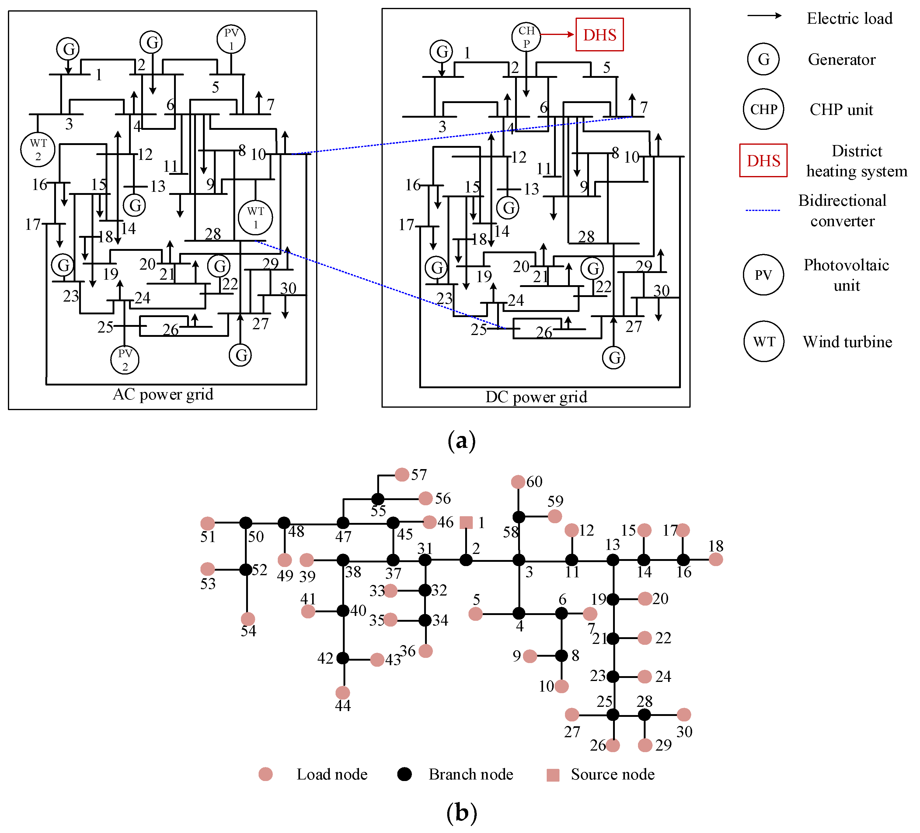
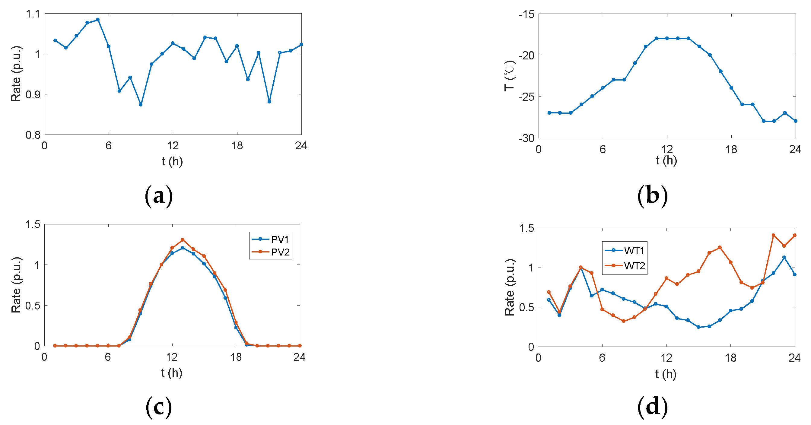
4.1. System Description

To evaluate the effectiveness of the proposed economic dispatch method, numerical simulations are conducted in an AC/DC power system with DHS, PV, and WT integration, as depicted in Figure 2. The AC and DC power systems share the same structure, which is derived from the IEEE 30-bus test system [7]. Buses 10 and 28 in the AC power system are connected to buses 7 and 26 in the DC power system through the bidirectional converters, respectively. All the data are the same as those in the IEEE 30-bus test system. Furthermore, a real-world 60-node HS in China is coupled with the DC power system through a CHP unit at bus 2, as illustrated in Figure 2b. In the AC power system, two PVs are integrated at buses 5 and 25, while two WTs are integrated at buses 3 and 10.

The variations in electric load, ambient temperature, maximum active power output of the PV units, and WTs are provided in Figure 3. The basic electric load distribution is the same as that in IEEE 30-bus test system; the basic PV’s and WT’s output is 5 MW. Both ambient temperature and electric load variation rates are given as known conditions, along with the maximum active power output of the PV units and WTs. All the simulations are performed on a PC with Intel i7 and 8 GB RAM and coded by Matlab 2021b. The economic dispatch problem is solved using IPOPT, which is widely used commercial software for large-scale nonlinear optimization problems. The simulation period is 24 h, with a time interval of 1 h.

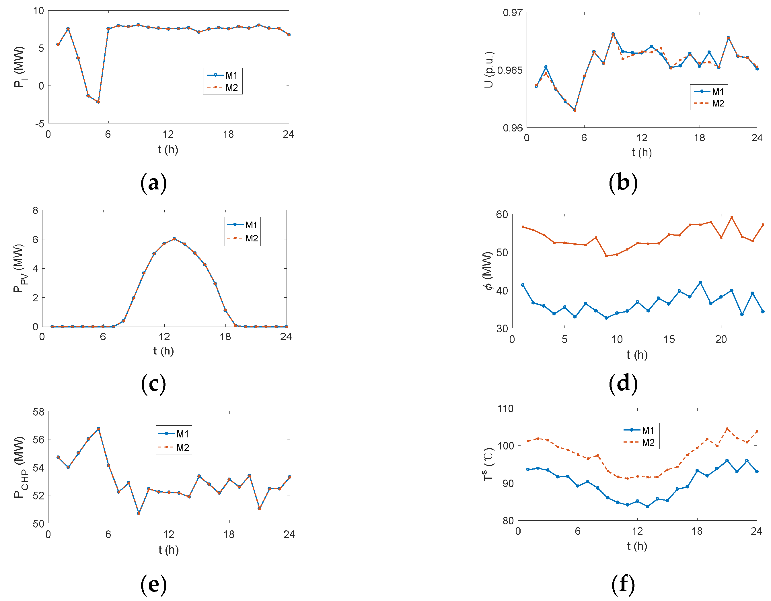
4.2. Verification of Thermal Dynamics

In this section, the effectiveness of the proposed optimization model is verified by comparing it with two other models: (M1) AC/DC power system model with the FAM for the DHS (method proposed in this paper) and (M2) AC/DC power system model with the node method (NM) for the DHS [21]. The results are summarized in Figure 4 and

Table 1. Results comparison between M1 and M2.

Model	Cp/USD	Cϕ/USD	CWT/USD	CPV/USD	C/USD	Time/s
M1	26,761	2093	599.13	304.22	29,757.35	74
M2	26,761	3484	599.13	304.22	31,148.35	129

.

According to Table 1, the optimization results for M1 and M2 are nearly identical, with the main differences observed in the results for the DHS and DC power system. From the perspective of operational cost, the costs associated with power generation, renewable maintenance, and abandonment are similar in both models. However, there is a significant difference in the cost of DHS operation. This difference arises due to the different modeling methods employed for the DHS in M1 and M2.

In the designed conditions, the time interval is much larger than the maximum time delay of the DHS. Consequently, the initial condition does not impose constraints on the early-stage optimization in the NM, leading to approximation errors that scale with the time interval. On the other hand, the FAM avoids introducing additional errors when transforming PDEs into algebraic equations. In the FAM, the early-stage operation is determined by the initial condition and the CHP unit only needs to maintain a lower output to ensure security. Therefore, the output thermal power of the CHP unit is lower, as shown in Figure 4d. However, the electric output of the CHP unit can still be adjusted within a large range and the AC/DC power system is only slightly affected, as shown in Figure 4e. As a result, the state distribution in the AC/DC power system and the renewables in the two models are similar, as shown in Figure 4a–c, which further indicates the superiority of the FAM in terms of accuracy.

In terms of efficiency, the solution times for M1 and M2 are 74 s and 129 s, respectively, highlighting the superior efficiency of the FAM for economic dispatch for the power system with multi-energy integration. This can be attributed to the avoidance of discretization and the associated variables in the FAM. Conversely, the discretization in the NM leads to a large number of discrete variables and equality constraints in the optimization model, making the problem more complex. Therefore, to achieve higher efficiency and accuracy, the subsequent simulations are performed based on M1.

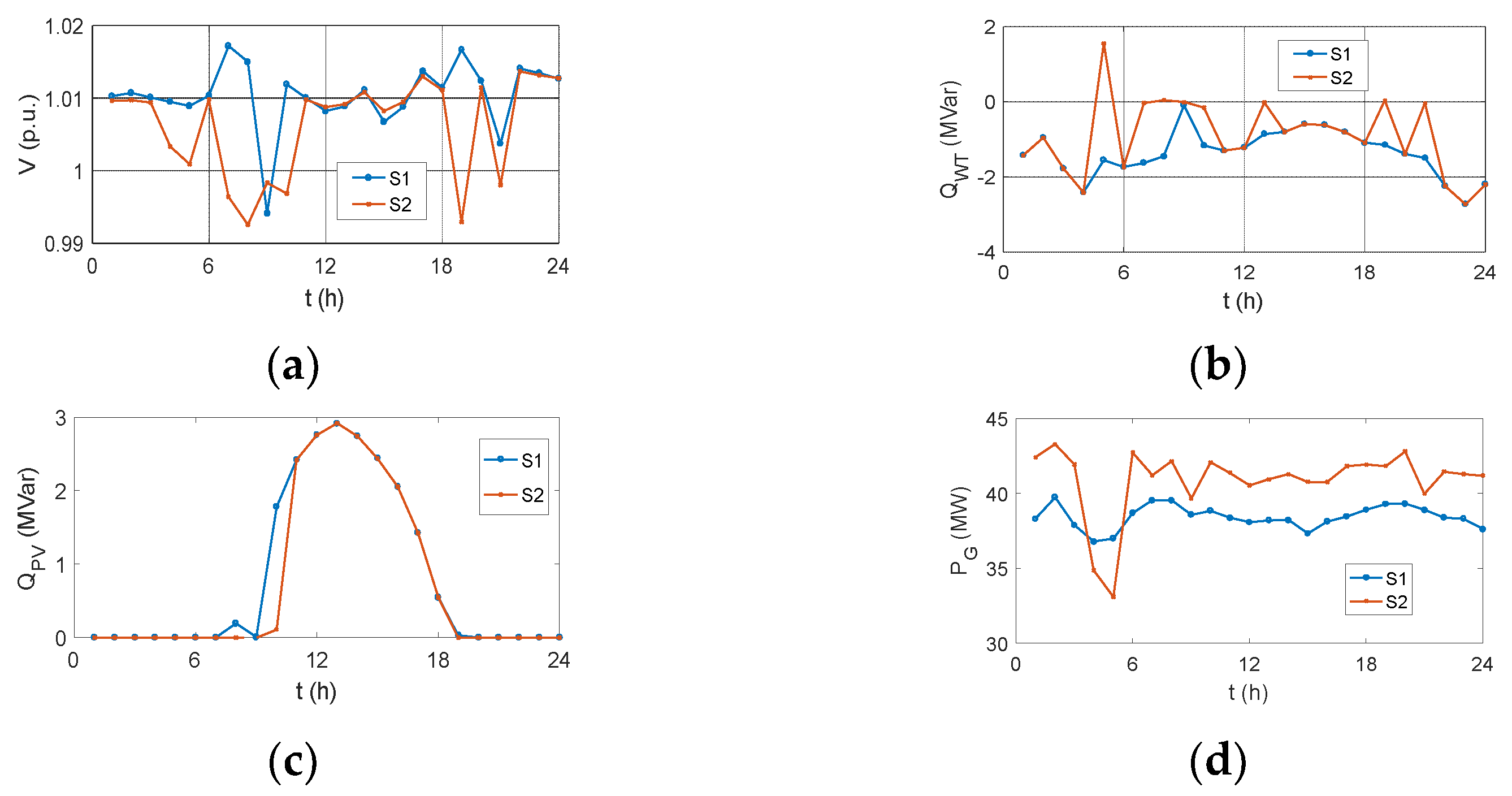
4.3. Influence of AC and DC Power System Interaction

In this section, we analyze the impact of AC/DC power system interaction on renewable consumption and operational cost through two scenarios.

In Scenario 1 (S1), we consider an AC/DC power system model and the FAM for the DHS. This scenario aligns with Model 1 (M1) in Section 4.2 and represents the proposed method in this paper.

In Scenario 2 (S2), we also utilize an AC/DC power system model [12,20] and FAM for DHS, but specifically exclude the interaction between the AC and DC power systems. The optimization period spans 24 h with a time interval of 1 h.

Table 2. Results comparison between S1 and S2.

Model	Cp/USD	Cϕ/USD	CWT/USD	CPV/USD	C/USD	Time/s
S1	26,761	2093	599.13	304.22	29,757.35	74
S2	26,869	2093	599.13	304.22	29,865.35	79

provides a summary of the solution time and operational costs for the different scenarios, while Figure 5 illustrates the optimized results.

Based on the results presented in Figure 5 and Table 2, we observe a slight difference in the optimized operational costs between the two scenarios. The dispatched results in the DHS varies. However, the variation is comparatively smaller compared with the feasible region; the electric power can still be adjusted in a certain region. Thus, the dispatched results in the power system are almost the same in different scenarios, causing the similar renewable energy output. Moreover, a more significant disparity emerges in the state distribution of the AC and DC power systems. The primary discrepancy arises from the generation cost. In S2, where the AC and DC power systems operate independently, there is no external power generation involved in the active–reactive power optimization. Conversely, in S1, the interaction between the AC and DC power systems introduces additional adjustable resources for power optimization beyond the optimization of internal generators. Consequently, the state distribution in S2 can be further optimized by considering the interactive power flow, resulting in an additional 0.4% reduction in the total operational cost. As the interactive capacity between the AC and DC power systems increases, it is expected that this improvement can be further enhanced.

Regarding the state distribution, Figure 5b demonstrates that, in S1, the WT at bus 10 primarily functions as a reactive power source and contributes to voltage regulation. However, in S2, the WT sometimes acts as a reactive power load. Consequently, the voltage level in S1 is higher compared to S2, as depicted in Figure 5a. Furthermore, based on the findings in Figure 4a, it is evident that the active power flow is transferred from the AC power system to the DC power system. As a result, the generators in S1 need to maintain a higher output to accommodate this power transfer. Conversely, in S2, the DC power system only needs to balance its internal load requirements, necessitating a lower output from the generators. This comparison is illustrated in Figure 4d.

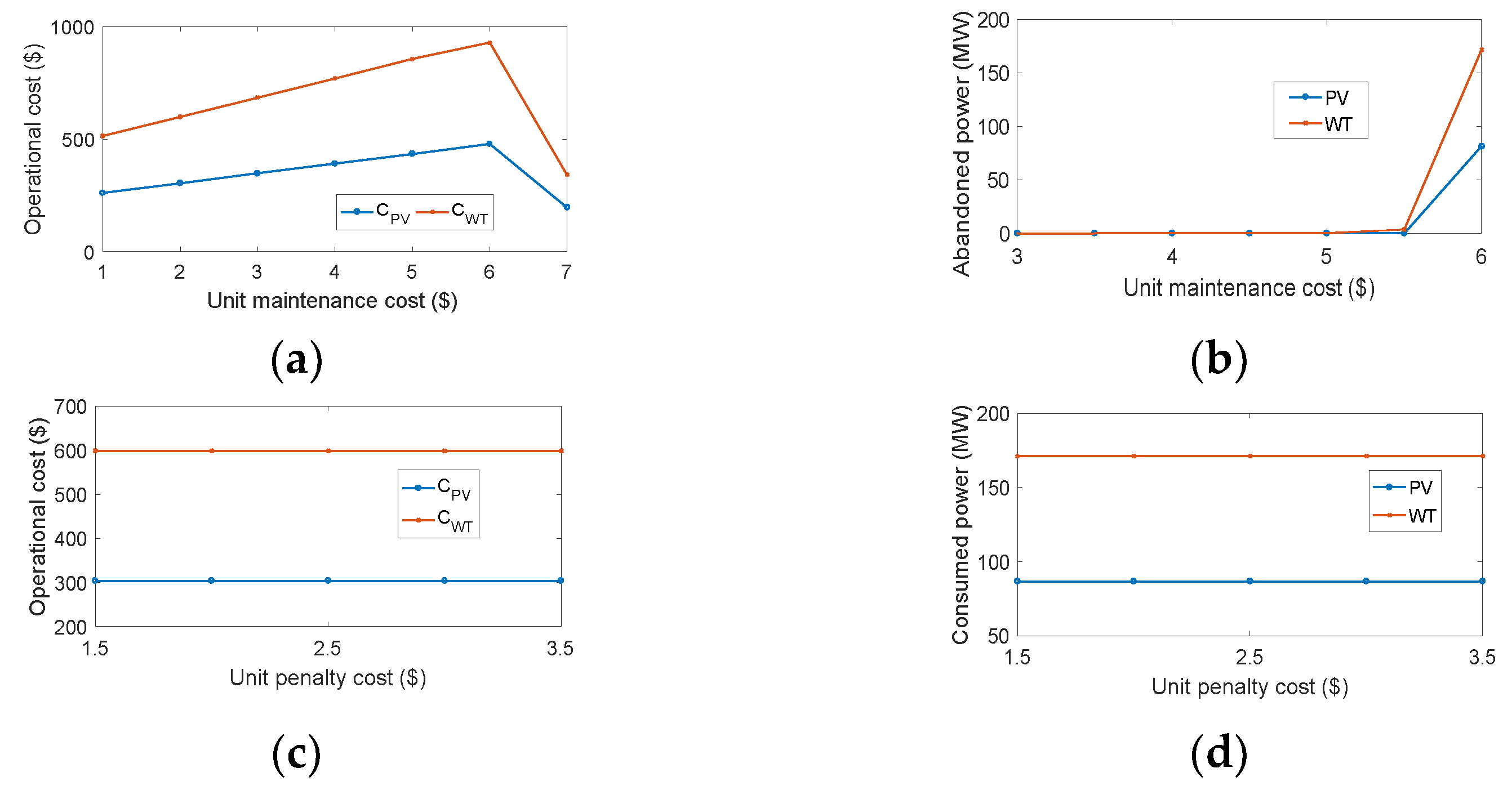
4.4. Influence of Unit Cost of Renewable Maintenance and Abandonment

In this section, we examine the impact of the unit cost of maintenance and abandonment for renewables on the operation of the AC/DC power system. The AC/DC power system model considering the DHS and renewable integration used in this section is our proposed method, and the various simulation results between different results are caused by different settings of unit cost of renewable maintenance and abandonment. Figure 6a,b illustrates the relationship between the total renewable consumption and the corresponding maintenance cost, with a constant unit penalty for abandonment.

The figure demonstrates that, initially, the operational cost scales proportionally with the unit cost of renewables’ maintenance. However, once the unit cost of maintenance reaches 6 USD/MW, the operator prefers to utilize traditional generators and accept the penalty associated with renewable abandonment. Consequently, the cost of utilizing renewables starts to decrease, as depicted in Figure 6a. Simultaneously, the abandoned renewable quantity remains at 0 until the unit cost of maintenance reaches 6 USD/MW, after which it increases sharply, as shown in Figure 6b.

Additionally, Figure 6c,d present the relationship between the total renewable consumption and the corresponding abandonment cost, assuming a constant unit cost of renewables’ maintenance. Notably, the operational costs and renewable consumption remain unchanged, regardless of the abandonment penalty. This can be attributed to the fact that the maintenance cost of renewables, set at 3 USD/MW, is lower than that of traditional generators. Therefore, the operator prefers to maximize the consumption of renewables to minimize the overall cost.

Overall, these findings indicate that the unit cost of maintenance and abandonment significantly impacts the operational decisions regarding renewable consumption and cost optimization in the AC/DC power system.

5. Conclusions

This paper has investigated the economic dispatch of the AC/DC power system, considering the integration of multi-energy sources and renewables. Throughout the study, the following key contributions have been made.

(1)

An improved DC power flow model and a fully analytical method is adopted to characterize the AC/DC power system considering DHS and renewable integration. The proposed model is more comprehensive and accurate.

(2)

A novel economic dispatch method for the coordinated operation of the active–reactive power, renewable energy, and the multi-energy flow is proposed, which fully explores the ability of the power system to promote renewable consumption and improve the operation economy.

The simulations conducted in the case study have validated the accuracy of the proposed model. The results have demonstrated that the interaction between the AC and DC power systems can enhance voltage levels, while the operational costs of renewables exert significant influences on the overall power system operation.

Looking ahead, future research efforts will be directed towards further advancing the modeling of the interaction between the AC and DC power systems. This will enable more comprehensive and refined economic dispatch in the AC/DC power system, thereby addressing the evolving complexities posed by the integration of renewable energy sources. Overall, the findings presented in this paper contribute to the understanding of economic dispatch in the AC/DC power system and pave the way for future advancements in the field.

References

1. Zhang, S.; Gu, W.; Zhang, X.-P.; Lu, H.; Yu, R.; Qiu, H.; Lu, S. Dynamic Modeling and Simulation of Integrated Electricity and Gas Systems. IEEE Trans. Smart Grid. 2023, 14, 1011–1026. [Google Scholar] [CrossRef]
2. Asensio, M.; Munoz-Delgado, G.; Contreras, J. Bi-Level Approach to Distribution Network and Renewable Energy Expansion Planning Considering Demand Response. IEEE Trans. Power Syst. 2017, 32, 4298–4309. [Google Scholar] [CrossRef]
3. Cruz, M.R.; Fitiwi, D.Z.; Santos, S.F.; Catalão, J.P. A comprehensive survey of flexibility options for supporting the low-carbon energy future. Renew. Sustain. Energy Rev. 2018, 97, 338–353. [Google Scholar] [CrossRef]
4. Mesanovic, A.; Munz, U.; Ebenbauer, C. Robust Optimal Power Flow for Mixed AC/DC Transmission Systems with Volatile Renewables. IEEE Trans. Power Syst. 2018, 33, 5171–5182. [Google Scholar] [CrossRef]
5. Zhou, M.; Zhai, J.; Li, G.; Ren, J. Distributed dispatch approach for bulk AC/DC hybrid systems with high wind power penetration. IEEE Trans. Power Syst. 2018, 33, 3325–3336. [Google Scholar] [CrossRef]
6. Ramsebner, J.; Haas, R.; Auer, H.; Ajanovic, A.; Gawlik, W.; Maier, C.; Nemec-Begluk, S.; Nacht, T.; Puchegger, M. From single to multi-energy and hybrid grids: Historic growth and future vision. Renew. Sustain. Energy Rev. 2021, 151, 111520. [Google Scholar] [CrossRef]
7. Zhang, S.; Gu, W.; Yao, S.; Lu, S.; Zhou, S.; Wu, Z. Partitional Decoupling Method for Fast Calculation of Energy Flow in a Large-Scale Heat and Electricity Integrated Energy System. IEEE Trans. Sustain. Energy 2020, 12, 501–513. [Google Scholar] [CrossRef]
8. Eajal, A.A.; Abdelwahed, M.A.; El-Saadany, E.F.; Ponnambalam, K. A unified approach to the power flow analysis of AC/DC hybrid microgrids. IEEE Trans. Sust. Energy 2016, 7, 1145–1158. [Google Scholar] [CrossRef]
9. Baradar, M.; Hesamzadeh, M.R.; Ghandhari, M. Second-Order Cone Programming for Optimal Power Flow in VSC-Type AC-DC Grids. IEEE Trans. Power Syst. 2013, 28, 4282–4291. [Google Scholar] [CrossRef]
10. Bahrami, S.; Therrien, F.; Wong, V.W.; Jatskevich, J. Semidefinite Relaxation of Optimal Power Flow for AC–DC Grids. IEEE Trans. Power Syst. 2017, 32, 289–304. [Google Scholar] [CrossRef]
11. Feng, W.; Tjernberg, L.B.; Mannikoff, A.; Bergman, A. A new approach for benefit evaluation of multi-terminal VSC-HVDC using a proposed mixed AC/DC optimal power flow. IEEE Trans. Power Deliv. 2014, 29, 432–443. [Google Scholar] [CrossRef]
12. Yang, Z.; Zhong, H.; Bose, A.; Zheng, T.; Xia, Q.; Kang, C. A Linearized OPF Model with Reactive Power and Voltage Magnitude: A Pathway to Improve the MW-Only DC OPF. IEEE Trans. Power Syst. 2017, 33, 1734–1745. [Google Scholar] [CrossRef]
13. Xu, F.; Tu, M.; Li, L.; Zhang, Y.; Leng, Y.; Chang, L. Scheduling model and solution of integrated power generation in power grid for clean energy accommodation. Autom. Electr. Power Systems 2019, 43, 185–193. [Google Scholar]
14. Li, Z.; Wu, L.; Xu, Y.; Wang, L.; Yang, N. Distributed tri-layer risk-averse stochastic game approach for energy trading among multi-energy microgrids. Appl. Energy 2023, 331, 185–193. [Google Scholar] [CrossRef]
15. Yu, J.; Dai, W.; Li, W.; Liu, X.; Liu, J. Optimal Reactive Power Flow of Interconnected Power System Based on Static Equivalent Method Using Border PMU Measurements. IEEE Trans. Power Syst. 2018, 33, 421–429. [Google Scholar] [CrossRef]
16. Zhang, H.; Zhang, S. A new strategy of HVDC operation for maximizing renewable energy accommodation. In Proceedings of the 2017 IEEE Power & Energy Society General Meeting, Chicago, IL, USA, 16–20 July 2017; pp. 1–6. [Google Scholar]
17. Zhang, X.; Tomsovic, K.; Dimitrovski, A. Security Constrained Multi-Stage Transmission Expansion Planning Considering a Continuously Variable Series Reactor. IEEE Trans. Power Syst. 2017, 32, 4442–4450. [Google Scholar] [CrossRef]
18. Jiang, T.; Dong, X.; Zhang, R.; Li, X.; Chen, H.; Li, G. Active-reactive power scheduling of integrated electricity-gas network with multi-microgrids. Front. Energy 2022, 17, 251–265. [Google Scholar] [CrossRef]
19. Zhang, H.; Qiu, X.; Zhou, S.; Liu, M.; Zhao, Y. Coordinated active-reactive optimization model for IEGES considering reactive power support by gas-fired turbine. Electr. Drive 2021, 51, 52–58. [Google Scholar]
20. Zhang, S.; Gu, W.; Zhang, X.-P.; Lu, H.; Lu, S.; Yu, R.; Qiu, H. Fully analytical model of heating networks for integrated energy systems. Appl. Energy 2022, 327, 120081. [Google Scholar] [CrossRef]
21. Li, Z.; Xu, Y.; Wang, P.; Xiao, G. Coordinated preparation and recovery of a post-disaster multi-energy distribution system considering thermal inertia and diverse uncertainties. Appl. Energy 2023, 336, 120736. [Google Scholar] [CrossRef]
22. Zhang, S.; Gu, W.; Wang, J.; Zhang, X.-P.; Meng, X.; Lu, S.; Pan, G.; Ding, S. Steady-state Security Region of Integrated Energy System Considering Thermal Dynamics. IEEE Trans. Power Syst. 2023, 1–15. [Google Scholar] [CrossRef]
23. Wu, Z.; Wang, Y.; You, S.; Zhang, H.; Zheng, X.; Guo, J.; Wei, S. Thermo-economic analysis of composite district heating substation with absorption heat pump. Appl. Therm. Eng. 2019, 166, 114659. [Google Scholar] [CrossRef]
24. Wang, Z.; Huang, W.; Cai, X. Security region of integrated heat and electricity system considering thermal dynamics. Front. Energy Res. 2022, 10. [Google Scholar] [CrossRef]
Figure 1. Diagram of AC/DC power system.
Processes 11 02522 g001
Figure 2. Sketches of systems in case study. (a) Sketch of the AC/DC power system. (b) Sketch of the 60-node DHS [23,24].
Processes 11 02522 g002
Figure 3. Variation rate in case study. (a) Electric load rate. (b) Ambient temperature. (c) PV units’ output rate. (d) WTs’ output rate [24].
Processes 11 02522 g003
Figure 4. Optimization comparisons between two models. (a) Pl,28,25 in AC/DC power system; (b) U5 in DC power system; (c) PPV at bus 5 in AC power grid; (d) ϕchp; (e) Pchp; (f) Ts at node 1.
Processes 11 02522 g004
Figure 5. Optimization comparisons between two scenarios. (a) U12 in AC power system; (b) QWT at bus 10 in AC power system; (c) QPV at bus 25 in AC power system; (d) PG at bus 1 in DC power system.
Processes 11 02522 g005
Figure 6. Influence of the renewables’ maintenance and penalty costs. (a) Operational cost with μPV/WT. (b) Abandoned renewables with μPV/WT. (c) Operational cost with αPV/WT. (d) Consumed renewables with αPV/WT.
Processes 11 02522 g006