New Technology and Method for Monitoring the Status of Power Systems to Improve Power Quality—A Case Study

Abstract

The identification and analysis of harmonics, frequency, and transient events are essential today. It is necessary to have available data relating to harmonics, frequency, and transient events to understand power systems and their proper control and analysis. Power quality monitoring is the first step in identifying power quality disturbances and reducing them and, as a result, improving the performance of the power system. In this paper, while presenting different methods for measuring these quantities, we have made some corrections to them. These reforms have been obtained through the analysis of power network signals. Finally, we introduce a new monitoring system capable of measuring harmonics, frequency, and transient events in the network. In addition, these values are provided for online and offline calculations of harmonics, frequency, and transient events. In this paper, two new and practical methods of the “algebraic method” are used to calculate network harmonics and wavelet transform to calculate transient modes in the network. Furthermore, the proposed monitoring system is able to reduce the amount of data-storage memory. The results of the simulations performed in this article show the superiority of using the new method presented for online and offline monitoring of power quality in electric power systems.

1. Introduction

The complexity of power grids has increased rapidly in recent decades. To know the different conditions governing the power grid, we must have the ability to measure its electrical quantities [1]. For this purpose, many measurement methods have been provided. The important point, in this case, is to provide the possibility of fast and online analysis of network quantities and harmonics in the power grid [2]. Accurately determining the frequency of the power grid today has become more difficult because of the presence of harmonics and other noises. Because it is difficult to maintain the dynamic balance of power systems in the current conditions that are expanding day by day, the frequency fluctuates around the nominal frequency. In addition, these frequency fluctuations are closely related to the dynamic states of the power grid. Therefore, real-time monitoring and measurement of the power grid frequency is also very important. This importance increases especially with the addition of harmonics to the power grid [3,4]. One of the main issues for industrial factories is how to deal with power grid disturbances. Power quality problems determine the degree of sensitivity of measurement equipment and provide valuable results.. This importance is due to the fact that some disturbances (such as a voltage drop of more than 30% in a short period of time) cause an interruption in the operation of controllers and relays, which makes the importance of qualitative analysis of power systems clearer [5]. In order to improve power quality, sources of error and disturbance should be identified and controlled. This action can be completed by sequentially performing error detection, recording the location and time of error occurrence, and classifying the errors. For this purpose, it is necessary to place suitable sensors on the network lines and identify the data received from them using suitable tools in real time [6]. In order to achieve this purpose, a powerful mathematical analysis tool is needed to simultaneously provide different analyses of the quality issues of the power system both in the time domain and in the frequency domain.

Among the factors that increase the importance of studying harmonics in the power network are the following: increasing the application of power electronics devices that have voltage and currents with non-linear characteristics and cause harmonics in the power network; increasing the shunt capacitor banks to correct the power factor and regulate the voltage range also increases the level of harmonics; and reducing the equipment design margin, which means that the equipment becomes more sensitive to voltage and current harmonics, harmonics have adverse effects on power network equipment and loads.

Harmonic disturbances usually appear in frequencies other than the main frequency of the network (but not always), and they often result from the non-linear operation of the mentioned factors in a permanent state and cause the collapse of the network. Here, the collapse of the network means the creation of unacceptable conditions for its network voltages and currents [7]. This definition is able to include all the errors and wrong operations and unwanted torques created in the shaft of electric machines. Except in very exceptional cases, common measuring devices and methods are not able to detect the number of harmonics or their different effects on the power system [8].

In this research, after reviewing the previous articles in this field, we present the statement of the proposed strategy.

This paper, considering the problems of power quality monitoring, especially in the online field, presents a new plan to solve these problems using the new algebraic method and wavelet transform.

Two methods are provided to identify transient states: One is performed using the derivative of the signal, and the other is conducted with the help of a new signal-processing technique called wavelet transform (which has been “used recently”). Finally, a monitoring system is proposed that is capable of identifying harmonics, frequency, and transient modes for real-time and offline analysis.

In order to be able to analyze the signal information offline, it is necessary to provide the possibility of storing this information in the memory. In this case, it is necessary to compress this information before saving. Some methods for compressing transients and steady states are mentioned. By applying these methods, information is compressed more than 40 times. In this system, with the new compression technique, the amount of memory needed to store the monitored data (for offline analysis) has been greatly reduced.

1.1. Background

In [9], the authors presented the frequency by calculating the phase voltage in quasi-steady and rotating frames with the DFT technique and regression relations. Because of the use of the DFT technique, this algorithm is inherently insensitive to network harmonics but is vulnerable to noise. Moreover, in this method, a wide measurement window is needed when measuring small frequency changes.

In [10], they used the Kalman filter to measure the frequency, and the method they used was able to remove the noise well, but it could not adequately consider the performance of harmonics.

In [11], the authors calculated the power grid frequency using the least-squares technique. However, their method was sensitive to both noise and network harmonics.

In [12], the frequency was measured using DSP and quadratic sampling data. In this paper, the authors removed the harmonics and the DC component of the grid voltage using a median filter.

In [13], the author defined the instantaneous frequency as the angular velocity of the spatial phasor of the voltage. He obtained good results, but the technique he used was very complicated.

In [14], the description of power quality monitoring (PQM) and the examination of the four main methods of PQM placement, which include monitor access area, coverage and packaging, graph theory, and multivariate regression, were discussed. In addition, the concepts, advantages, and disadvantages of each method were discussed.

Various methods have been presented in this field, including discrete Fourier transform (DFT) and fast Fourier transform (FFT). One of the main reasons for paying special attention to the FFT technique is its lesser need for computing devices. This feature is obtained by removing the additional coefficients of the differential equation of the signal under analysis. However, there are limitations in this method. One of is causing disruptions in the proper selection of data windows. One of these limitations is leakage. Leakage occurs when the data window used for the technique FFT does not contain a precise interval of integers of frequency cycles. Because this method depends on the information windows of the signal under monitoring, due to the inevitable changes in the signal frequency, the problem of leakage will therefore always exist in this method [15].

In addition, the FFT technique has inherent limitations in terms of resolution. Today, improvements have been made to the FFT technique that have improved the mentioned issues to a great extent. Among them, it is possible to mention the selection of information windows based on the detection of crossing the zero level of the signal. Although the use of zero-level detection methods is simple and completely reliable (even for low-level noise pollution conditions), if the range of high-order harmonics of the signal is significant, the accuracy of this method is significantly reduced. Another way to evaluate the monitored signal is to use Taylor series techniques. This method also suffers from the same limitations that existed in detecting the crossing of the zero level [16,17].

There are also some methods that use the FFT technique as a starting point to estimate the phase of the main harmonic, and then the frequency of the main harmonic is calculated based on the change in phase angle shifting. This method is successful only when the changes in the main frequency are insignificant. Otherwise, as mentioned earlier, the leakage problem causes a gross error in the initial values of the central harmonic phase obtained from the technique FFT. These methods have also been improved by the least squares algorithm or using the Kalman filter. In most common methods, the main harmonic is the primary basis. Therefore, if there are many other harmonics in the signal under analysis, these harmonics can affect the results of these methods [18].

The latest method of monitoring electrical quantities uses non-linear methods to follow the signal under monitoring. Using the Newton iteration method and combining it with the least square method is one of these non-linear methods. Nevertheless, this method is computationally intensive, and therefore, several processors must be used in parallel to perform real-time analysis. Artificial neural networks can be used to increase the speed of calculations. It should be remembered that the use of neural networks in monitoring harmonics is not a new concept. This method can provide accurate results of the conditions of network quantities, even if complete information about these quantities is not available [19].

But the new method presented in this article is the algebraic method which will be explained below. While this method is straightforward, it also solves many of the disadvantages of the standard DFT method. Also, in this article, the DFT method and the algebraic method mentioned, have been turned into reversible methods. Hence, their calculation speed is equal to the speed of the minimum gradient method solved with the help of Hopfield neural network.

To analyze transient states, Riberio was one of the first to use WT. He realized that the WT is easily able to separate the transient states and the primary states of the power network signals from each other, with the most minor parameters and the most accuracy, and he identifies them [20]. Later, people like Galli, Heydt, etc., used different types of WT for different cases of power network analysis. Even today, there are many articles about the different use cases of WT in the power network.

1.2. The Weaknesses of Previous Research and the Importance and Necessity of Research

In this section, the weaknesses of the proposed methods in previous many articles are explained. Classical artificial intelligence in previous articles in this field does not give importance to the aspects of system development (how knowledge structures are created and their changes over time). Through monitoring power quality disturbances, it is possible to examine the details of the disturbances and determine solutions to overcome the system’s power quality problems. The main part of power quality monitoring, which is very important and effective, is the identification and classification of power disturbance signals and requires signal processing techniques and machine learning tools (intelligent tools) [21,22]. Today, many studies have been published to classify power quality disorders. Each article has achieved different accuracies by using a particular diagnosis structure. The reality is that each diagnosis structure may have the desired answer for specific conditions and data. Therefore, comprehensive and efficient monitoring needs an automatic and intelligent framework to make the best decision among the candidate structures when necessary, according to the set goal [23]. The main problem in this field is the lack of comprehensiveness of the diagnosis system and not making a proper and timely decision in determining the structure of the optimal diagnosis. In the systems presented in the reference articles, the need for adaptability and flexibility to changing environmental conditions and changing the characteristics of the data in the database has not been considered. In many previous studies, there is no feature selection section (data mining) to improve the operation of the detection system. The performance of classification tools depends on several internal parameters, which have been set by trial and error in many previous articles. In many practical applications in this field, the accuracy and efficiency of existing methods are not suitable against different noise conditions and should be improved. In some articles, attempts have been made to improve the performance of these systems by using noise removal methods and adding new steps in the structure of the noise detection system, but these methods have not been well received due to their complexity and large number of calculations. And this research has led to new and advanced signal processing algorithms that are inherently robust to noise. In general, it can be said that in many previous studies, only the performance of an offline monitoring system has been investigated [24,25].

2. Frequency Monitoring Methods

In this section, several methods for measuring frequency are presented.

2.1. The Modified Technique of Crossing the Zero Level

The sampled voltage waveform can be formulated as follows [26,27]:

$$v\left(k\right)=v\left(kT\right)={\displaystyle \sum _{n=1}^{\infty }{V}_n\cos \left(n{\omega }_{0}kT+{\delta }_n\left(kT\right)\right)}$$

(1)

The data window $V\left[k\right]$ for M consecutive sample is defined as follows:

$$V\left[k\right]={\left[v\left(k+1\right),v\left(k+2\right),\cdots ,v\left(k+M\right),\right]}^T$$

(2)

The time to open the informational window is optional. The polynomial of degree Lth of $p_l\left(t\right)$ is assumed as follows [28]:

$$p_l\left(t\right)=a_0+a_{1}t+a_2{t}^2+\cdots +a_l{t}^l={\displaystyle \sum _{j=1}^l{a}_j{t}^j}$$

(3)

If each of the mentioned sentences is equal to the voltage at the moment t, and it can be written as:

$$\left[\begin{array}{l}1\left(k+1\right)T{\left(k+1\right)}^2{T}^2 \cdots {\left(k+1\right)}^l{T}^l\\ 1\left(k+2\right)T{\left(k+2\right)}^2{T}^2 \cdots {\left(k+2\right)}^l{T}^l\\ \hspace{1em}\hspace{1em}\cdots \\ 1\left(k+M\right)T{\left(k+M\right)}^2{T}^2 \cdots {\left(k+M\right)}^l{T}^l\end{array}\right]\left[\begin{array}{l}{a}_0\\ a_1\\ ⋮\\ a_l\end{array}\right]=V\left[k\right]$$

(4)

or as:

$$K\cdot a=V\left[k\right]\Rightarrow a={\left(K^{T}K\right)}^{-1}{K}^{T}V\left[k\right]$$

(5)

In this way, the voltage waveform can be calculated as a polynomial of degree l, in terms of the time variable and in the distance k to k + M. This means that:

$$v\left(t\right)=a_0+a_{1}t+a_2{t}^2+\cdots +a_l{t}^l\hspace{1em}for\hspace{1em}k\le t\le k+M$$

(6)

Usually, “l” is considered to be at most 3. In this case, for each M + 1 sample, V(t) is approximated by a new third-order function. The moment of crossing the zero level is between two sequences in which the sign changes. If these sequences are denoted by m and m + 1, then the relation (6) can be written as follows:

$$\begin{gathered} v\left(t\right)=a_0+a_{1}t+a_2{t}^2+\cdots +a_l{t}^l; \\ for m-\left[\frac{M+1}{2}\right]\le t\le \left(m-\left[\frac{M+1}{2}\right]\right)+M-1 \end{gathered}$$

(7)

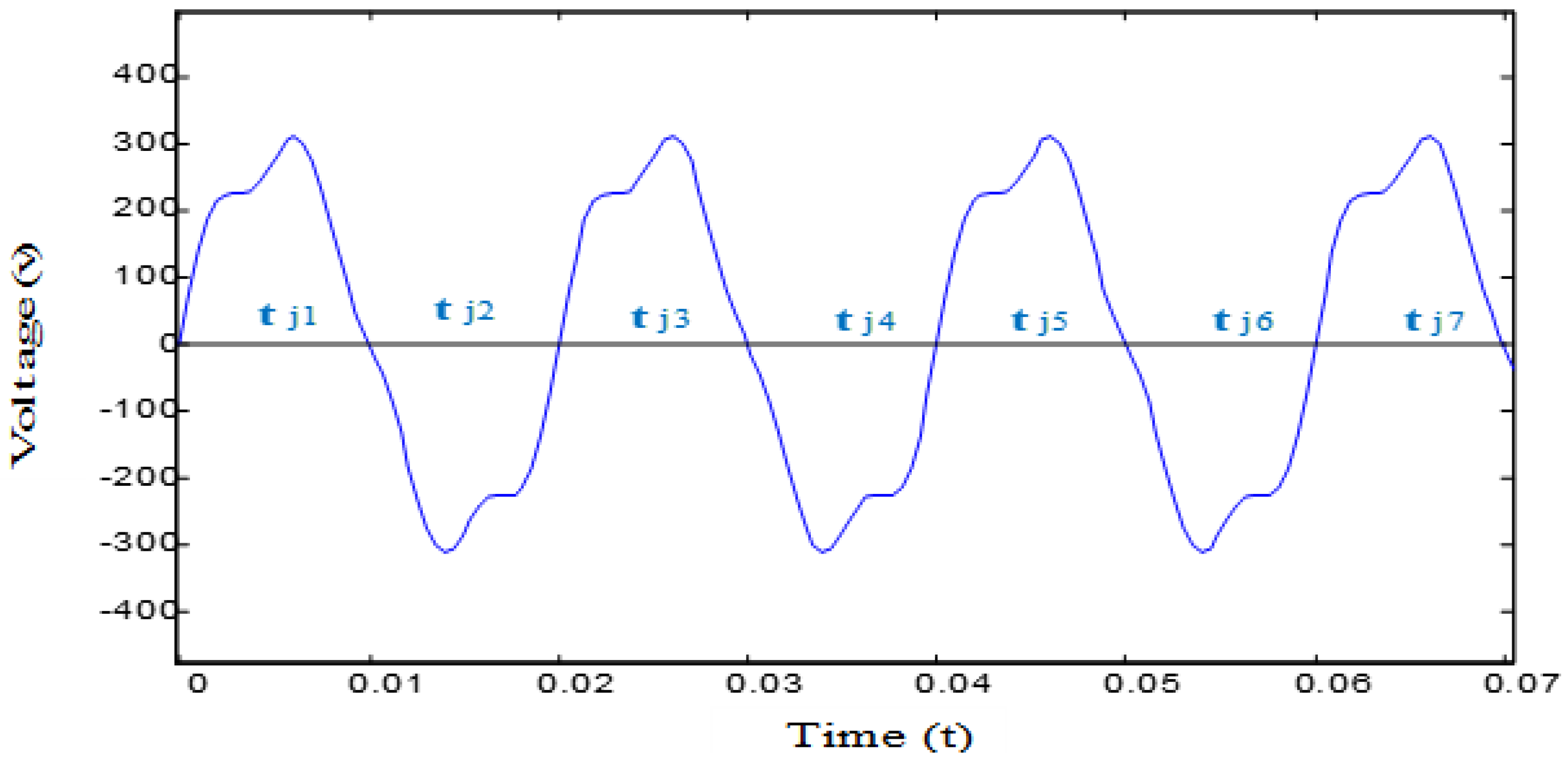
Now, if V(t) = 0 is solved for Equation (7), the time the curve crosses the zero level is calculated. In the same way, we calculate all the points crossing the zero level of the signal and call them in $\cdots ,t_{j_2},t_{j_1}$ in order, as in Figure 1:

Therefore, the period of the sampled signal in the Jth cycle is:

$$T_j=t_j-t_{j-2}\hspace{1em}for\hspace{1em}j\ge 3$$

(8)

Also, the frequency of this signal in the Jth cycle is calculated from the following equation:

$$f_j=\frac{1}{t_j-t_{j-2}}\hspace{1em}for\hspace{1em}j\ge 3$$

(9)

As seen in the above figure, it can be proved that the calculated frequency for almost “periodic” signals depends on the value of the DC level. Furthermore, if the waveform of the signal has a significant difference from one period to another, before calculating the crossing point of the zero level, the value of the DC level calculated in the previous period should be subtracted from the relation of the primary wave, and then the crossing point of the level zero measured the resulting signal, which is free of DC component.

2.2. DFT Method with Polynomial Approximation

The sampled voltage waveform can be formulated as follows [29]:

$$v\left(k\right)=v\left(kT\right)={\displaystyle \sum _{n=1}^{\infty }{V}_n\cos \left(n{\omega }_{0}kT+{\delta }_n\left(kT\right)\right)}$$

(10)

The data window $V\left[k\right]$ for M consecutive sample is defined as follows:

$$V\left[k\right]={\left[v\left(k+1\right),v\left(k+2\right),\cdots ,v\left(k+M\right),\right]}^T$$

(11)

The real and imaginary parts of the voltage phasor from the discrete Fourier transform relation are as follows:

$$\begin{array}{l}\Re \left\{{\tilde{V}}_1\left[k\right]\right\}=V_1\cos {\delta }_1=\frac{2}{N}{\displaystyle \sum _{j=1}^{N}v\left[k+j\right]\cos \left(\frac{2\left(k+1\right)\pi }{N}\right)}\\ \Im \left\{{\tilde{V}}_1\left[k\right]\right\}=V_1\cos {\delta }_1=\frac{2}{N}{\displaystyle \sum _{j=1}^{N}v\left[k+j\right]\sin \left(\frac{2\left(k+1\right)\pi }{N}\right)}\\ \Rightarrow {\tilde{V}}_1=V_1{e}^{j{\delta }_1} \end{array}$$

(12)

The mentioned method can be considered as a harmonic filter. If the phasor voltages of all three phases are available, the positive sequence phasor can be calculated from them follows:

$${\tilde{V}}_1\left[k\right]={\tilde{V}}_{1a}\left[k\right]+\alpha {\tilde{V}}_{1b}\left[k\right]+{\alpha }^2{\tilde{V}}_{1c}\left[k\right],\left(\alpha =e^{j2\pi /3}\right)$$

(13)

To calculate, $\delta \left[k\right]$, we consider it as the argument of ${\tilde{V}}_1\left[k\right]$ and consider a sliding data window as follows:

$$D\left[k\right]={\left[\delta \left[k+1\right]\delta \left[k+2\right]\cdots \delta \left[k+M\right]\right]}^T$$

(14)

Now, inside this window, the positive sequence phasor argument function of the voltage is approximated by a polynomial of the Lth degree.

$$\delta \left(t\right)=a_0+a_{1}t+\cdots +a_l{t}^l={\displaystyle \sum _{j=1}^l{a}_j{t}^j}$$

(15)

In this way, the instantaneous frequency of the voltage, which is the instantaneous derivative of its argument, can be calculated:

$$f\left(t\right)=\frac{1}{2\pi }\frac{d\delta \left(t\right)}{dt}=\frac{1}{2\pi }\left(a_1+2a_{2}t+\cdots +a_l{t}^{l-1}\right)$$

(16)

The discrete form of the relation (16) can also be written as follows:

$$f\left(k\right)=f\left(k\Delta t\right)=\frac{1}{2\pi }{\displaystyle \sum _{j=0}^{l-1}j{a}_j{\left(k\Delta t\right)}^{j-1}}$$

(17)

The frequency at the end of each data window should be calculated consecutively.

$$f\left[k+M\right]=\frac{1}{2\pi }{\displaystyle \sum _{j=0}^{l-1}j{a}_j{\left(\left[k+M\right]\Delta t\right)}^{j-1}}$$

(18)

It can be seen that the realization of the mentioned method in real time is straightforward. In this method, the DFT technique protects against harmonics, and the least square technique protects the system against noise. Therefore, noise and harmonics cannot have a great effect on the calculated frequency value. Nevertheless, it has a complex calculation method.

3. Power System Monitoring

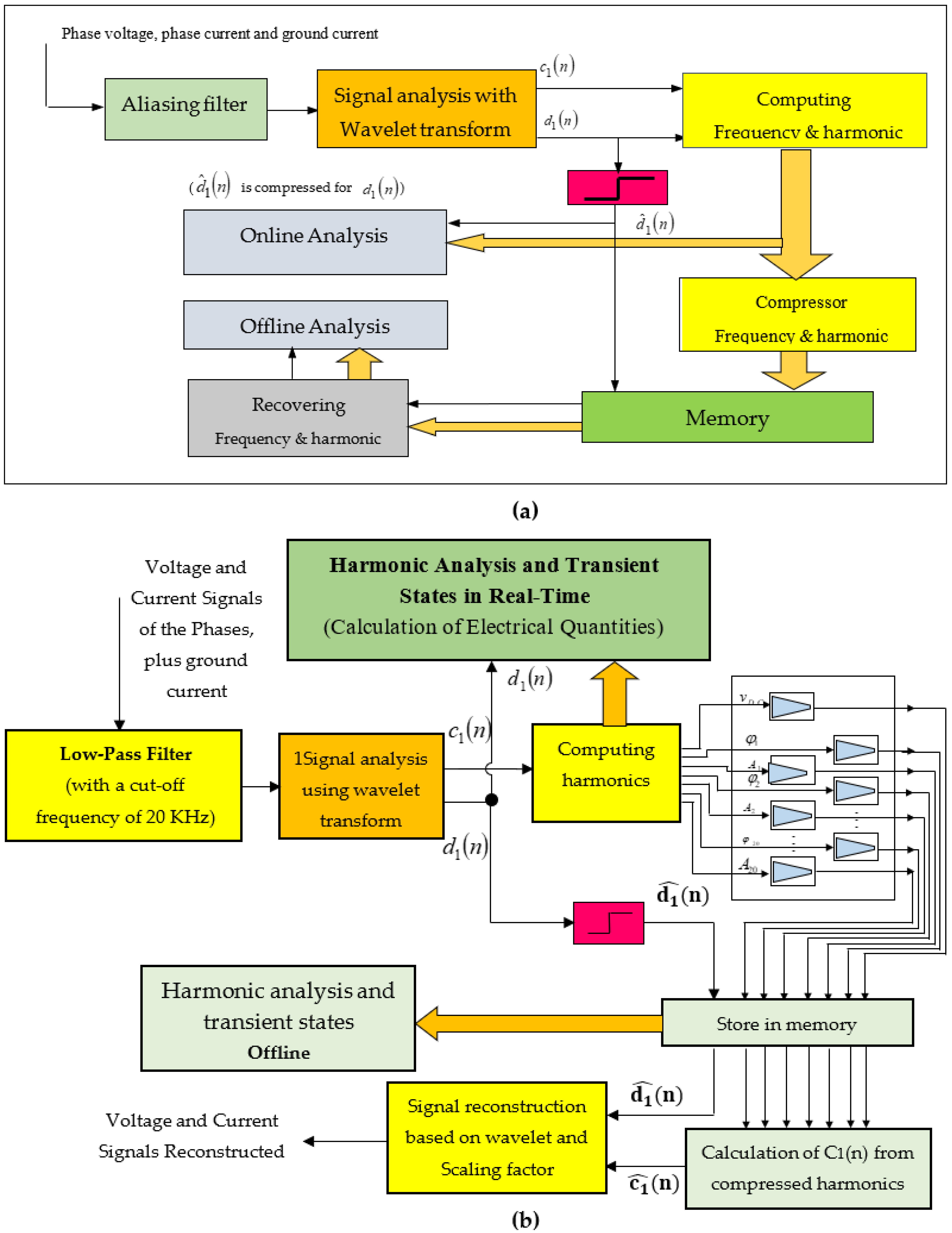
In this section, a new method for online and offline monitoring is presented using the mentioned methods for identifying transient states and harmonics. The basis of work in the aforementioned monitoring above system is as follows: First, the signal is passed through a low-pass filter with a cut-off frequency of 10 kHz to solve the aliasing problem. Then, it is sampled with a sampling frequency of 24 kHz (ensuring compliance with Nyquist’s theorem). Later, a wavelet stage is taken from the resulting discrete signal. The harmonics of the power network (in steady state) are always limited to less than the 20th order, and therefore, only samples of the signal are used to calculate the harmonics, and the distance between them is equal to 0.02/41 s [30]. In this system, the harmonics and the primary harmonic frequency are calculated in real time via the reversible algebraic method. Also, to identify transient states, two methods are presented here. Depending on the accuracy and sensitivity of the system, any of them can be used. For offline analysis, the monitoring system can compress and store the harmonics and transient states of the signal with a new technique (which will be explained below). The presented method in signal compression, in addition to being highly accurate, can significantly compress any original signal. The block diagram of the mentioned monitoring system is shown in Figure 2 and consists of the following components:

• Aliasing filter for removing aliasing problem.
• Sampler; with 24 kHz sampling, for sure of observing the Nyquist theorem.
• Subsystem WT with one level.
• Subsystem computation frequency and harmonic with zero crossing method and algebraic method.
• Frequency and harmonic compressor with the new method.
• Transient values (wavelet factor) compressor.
• Memory to store compressed variables (frequency, harmonic and transient values).
• A subsystem that includes recovery frequency and harmonic and transient values, with new methods and remarking signal monitoring.

3.1. Description of the System Scaling

3.1.1. Signal Analysis by Wavelet

The sampled signal is analyzed via the wavelet transform into the wavelet factor of the first level ($d_1$) and the scale factor of the first level ($c_1$).

3.1.2. Harmonic Calculation

The scaling factor of the first level is the parts of the low-frequency spectrum of the monitored signal. In other words, this coefficient includes the steady state of the waveform. Assuming that the harmonics of the signals are limited to the 20th order, it is possible to obtain the DC value and the amplitude and phase of the monitored signals with 41 samples of it in one period using the algebraic method.

Figure 3 shows sampled voltage signal, scaling factor ($c_1$), and wavelet factor ($d_1$), respectively. Let us suppose the signal $v\left(t\right)$ is calculated as shown below:

$$\begin{array}{l}v\left(t\right)=60+40\sin \left(2\pi \left(3\times 50\right)\hspace{0.17em}t\right)\hspace{0.17em}\\ +200p\left(t\right)\sin \left(2\pi \left(50\times 50\right)\hspace{0.17em}t\right)\end{array}$$

(19)

where: $p\left(t\right)=u\left(t-0.01\right)-u\left(t-0.011\right)$, and $u\left(t\right)$ is a unit function.

3.1.3. Algebraic Method for Calculation of Harmonic

The scaling factor $\left(c_1\right)$ shows a low-frequency spectrum of the monitoring signal. In other words, this coefficient shows the steady state of the monitoring signal. In this case, we can calculate the DC magnitude and phase harmonics of the monitoring signal with 41 samplings in one period. First, the momentary frequency is calculated by detected the zero crossing of $c_1$, and then the DC value, magnitude, and phase of harmonics are calculated via the algebraic method. The algebraic method, which has been presented for the time first in this paper, is confirmed based on solving of the algebraic equations obtained through the sampling of $c_1$ (when that rating frequency is constant) [30]. Thus, for this reason, we have called it the algebraic method, and we describe it in the following section. The waveform of the power network voltage in the presence of network harmonics can be written as follows:

$$v(k)=v_0+{\displaystyle \sum _{n\hspace{0.17em}=\hspace{0.17em}1}^N\left[a_n\hspace{0.17em}\cos \left(2\hspace{0.17em}\pi \hspace{0.17em}n\hspace{0.17em}f\hspace{0.17em}{T}_S\hspace{0.17em}k\right)+b_n\hspace{0.17em}\sin \left(2\hspace{0.17em}\pi \hspace{0.17em}n\hspace{0.17em}f\hspace{0.17em}{T}_S\hspace{0.17em}k\right)\right]}$$

(20)

In this equation, $f,\hspace{0.17em}k,\hspace{0.17em}v\left(k\right)$ are known. Thus, $\cos \left(2\hspace{0.17em}\pi \hspace{0.17em}n\hspace{0.17em}f\hspace{0.17em}{T}_S\hspace{0.17em}k\right)\hspace{0.17em},\hspace{0.17em}\sin \left(2\hspace{0.17em}\pi \hspace{0.17em}n\hspace{0.17em}f\hspace{0.17em}{T}_S\hspace{0.17em}k\right)$ are also known. We want calculate $a_n,\hspace{0.17em}{b}_n\hspace{0.17em}and\hspace{0.17em}{v}_{DC}$ [31]. It is observed that number of unknowns is $2N+1$ and that $N$ is the number of harmonics (or the last order harmonic in voltage). Because $\cos \left(2\hspace{0.17em}\pi \hspace{0.17em}n\hspace{0.17em}f\hspace{0.17em}{T}_S\hspace{0.17em}k\right)$ and $\sin \left(2\hspace{0.17em}\pi \hspace{0.17em}n\hspace{0.17em}f\hspace{0.17em}{T}_S\hspace{0.17em}k\right)$ are known, thus, Equation (21) can be classed as a linear equation on the basis of $a_n,\hspace{0.17em}{b}_n\hspace{0.17em}and\hspace{0.17em}{v}_{DC}$ variables. Thus, we can write the algebraic equation system with $2N+1$ unknowns and $2N+1$ linear equations for $2N+1$ samples of $v\left(t\right)$, in the form below:

$$V=A\hspace{0.17em}X$$

(21)

where

$$V=\left[\begin{array}{l}v\left(1\right)\\ v\left(2\right)\\ \hspace{0.17em}\hspace{0.17em}⋮\\ v\left(M\right)\end{array}\right]\hspace{0.17em}\hspace{0.17em}\hspace{0.17em},X=\left[\begin{array}{l}{v}_{DC}\\ a_1\\ \hspace{0.17em}\hspace{0.17em}⋮\\ a_n\\ b_1\\ \hspace{0.17em}\hspace{0.17em}⋮\\ b_n\end{array}\right], \begin{array}{l}v\left(k\right)=v\left(T_{S}k\right)\hspace{0.17em}\hspace{0.17em},\left(for\hspace{0.17em}k=1,\dots ,M\right)\\ and\hspace{0.17em}\hspace{0.17em}\hspace{0.17em}\hspace{0.17em}\hspace{0.17em}M=2N+1\end{array}$$

(22)

$$A_1=\left[\begin{array}{l}1\hspace{0.17em}\cos \left(2\pi f\left(1T_S\right)\right)\hspace{0.17em}\cdots \hspace{0.17em}\cos \left(2\pi f\left(1T_S\right)\right)\\ 1\hspace{0.17em}\cos \left(2\pi f\left(2T_S\right)\right)\hspace{0.17em}\cdots \hspace{0.17em}\cos \left(2\pi f\left(2T_S\right)\right)\\ \hspace{0.17em}\hspace{0.17em}\hspace{0.17em}\hspace{0.17em}\hspace{0.17em}\hspace{0.17em}\hspace{0.17em}\hspace{0.17em}\hspace{0.17em}\hspace{0.17em}\hspace{0.17em}\hspace{0.17em}\hspace{0.17em}\hspace{0.17em}\hspace{0.17em}\hspace{0.17em}\hspace{0.17em}\hspace{0.17em}\hspace{0.17em}\hspace{0.17em}\hspace{0.17em}⋮\\ 1\hspace{0.17em}\cos \left(2\pi f\left(M{T}_S\right)\right)\hspace{0.17em}\cdots \hspace{0.17em}\cos \left(2\pi f\left(M{T}_S\right)\right)\end{array}\right]$$

(23)

and

$$\begin{array}{l}{A}_2=\left[\begin{array}{l}\sin \left(2\pi f\left(1T_S\right)\right)\hspace{0.17em}\cdots \hspace{0.17em}\sin \left(2\pi f\left(1T_S\right)\right)\\ \sin \left(2\pi f\left(2T_S\right)\right)\hspace{0.17em}\cdots \hspace{0.17em}\sin \left(2\pi f\left(2T_S\right)\right)\\ \hspace{0.17em}\hspace{0.17em}\hspace{0.17em}\hspace{0.17em}\hspace{0.17em}\hspace{0.17em}\hspace{0.17em}\hspace{0.17em}\hspace{0.17em}\hspace{0.17em}\hspace{0.17em}\hspace{0.17em}\hspace{0.17em}\hspace{0.17em}\hspace{0.17em}\hspace{0.17em}\hspace{0.17em}\hspace{0.17em}\hspace{0.17em}\hspace{0.17em}⋮\\ \sin \left(2\pi f\left(M{T}_S\right)\right)\hspace{0.17em}\cdots \hspace{0.17em}\sin \left(2\pi f\left(M{T}_S\right)\right)\end{array}\right]\\ A=\left[A_1\hspace{0.17em},\hspace{0.17em}{A}_2\right]\end{array}$$

(24)

Because $A$ is constant, $A^{-1}$ is also constant. Thus, it is enough to just calculate $A$ one time and then $A^{-1}$, for solving Equation (1) [32,33].

$$\hspace{0.17em}\hspace{0.17em}\hspace{0.17em}\left[\begin{array}{l}{v}_{DC}\\ a_1\\ \hspace{0.17em}\hspace{0.17em}⋮\\ a_n\\ b_1\\ \hspace{0.17em}\hspace{0.17em}⋮\\ b_n\end{array}\right]=A^{-1}\hspace{0.17em}\left[\begin{array}{l}v\left(1\right)\\ v\left(2\right)\\ \hspace{0.17em}\hspace{0.17em}\hspace{0.17em}⋮\hspace{0.17em}\hspace{0.17em}\\ \hspace{0.17em}\hspace{0.17em}\hspace{0.17em}⋮\\ \hspace{0.17em}\hspace{0.17em}\hspace{0.17em}⋮\\ \hspace{0.17em}\hspace{0.17em}\hspace{0.17em}⋮\hspace{0.17em}\\ v\left(M\right)\end{array}\right]$$

(25)

3.1.4. Recursive Algebraic Method

If $A^{-1}$ is written in the form below:

$$A^{-1}={\left[c_{i,j}\right]}_{2N+1,2N+1}\hspace{0.17em}\hspace{0.17em},\hspace{0.17em}\left(i,j=1,\cdots ,2N+1\right)$$

(26)

then from Equations (25) and (26), we have:

$$v_{DC}={\displaystyle \sum _{j=1}^{2N+1}{c}_{1,j}\hspace{0.17em}v\left(j\right)}\hspace{0.17em}\hspace{0.17em}\hspace{0.17em}$$

(27)

$$a_n={\displaystyle \sum _{j=1}^{2N+1}{c}_{n+1,j}\hspace{0.17em}v\left(j\right)}\hspace{0.17em}$$

(28)

$$b_n={\displaystyle \sum _{j=1}^{2N+1}{c}_{N+n+1,j}\hspace{0.17em}v\left(j\right)}\hspace{0.17em}$$

(29)

It is observed that for calculating $a_n,\hspace{0.17em}{b}_n$, and $\hspace{0.17em}{v}_{DC}$, it is required that we have completed one period of signal monitoring, and then it is necessary to perform a high volume of calculating for $a_n,\hspace{0.17em}{b}_n$, and $\hspace{0.17em}{v}_{DC}$. The reason for this is because for each variable, it is necessary to perform $2N+1$ sum operations and $2N+1$ multiple operations, and also, the number of variables is $2N+1$. In total, ${\left(2N+1\right)}^2$ operations of multiplication and addition should be performed. A method is presented here that divides these calculations among samplings. The method of performing the work is as follows: if the period we calculate the harmonics is the kth period, we can write [34]:

$$v_{DC}^k\left(j+1\right)=v_{DC}^k\left(j\right)+c_{1,j}\hspace{0.17em}v\left(j\right)$$

(30)

$$a_n^k\left(j+1\right)=a_n^k\left(j\right)+c_{n+1,j}\hspace{0.17em}v\left(j\right)$$

(31)

$$b_n^k\left(j+1\right)=b_n^k\left(j\right)+c_{N+n+1,j}\hspace{0.17em}v\left(j\right)$$

(32)

In the above relationships, $k$ is the period number, $i$ is the sample number in the kth period, n is the harmonics number, and N is the total number of harmonics. The number of samples in each period starts from one, and the initial values of the variables are one at the beginning of each period; this means that $v_{DC}^k\left(1\right)=a_n^k\left(1\right)=b_n^k\left(1\right)=0$.

It can be seen that after the 2N + 1 sample or after going through a period, the harmonics and the DC value of the signal are calculated [35]. Then, the sampling number $i$ is equal to zero, and one is added to the value of k (period number) so that the amount of harmonics in the next period is calculated in the same way. In this method, because the value of the variables in each sampling stage (in any period) depends on the value of the variable in the previous sampling stage (of the same period), it is called the recursive method.

3.1.5. Simulation of Algebraic Method

To show the ability of the algebraic method, we consider the voltage of the power system in the form below [36]:

$$\begin{array}{l}v\left(t\right)=60+300e^{-2t}\sin \left(2\pi 50\hspace{0.17em}t\right)+40\sin \left(2\pi \left(3\times 50\right)\hspace{0.17em}t\right)\hspace{0.17em}\\ +200p\left(t\right)\sin \left(2\pi \left(50\times 50\right)\hspace{0.17em}t\right)\end{array}$$

(33)

where $p\left(t\right)=u\left(t-0.01\right)-u\left(t-0.011\right)$. Moreover, $u\left(t\right)$ is a unit function.

The following figures show the simulation of voltage variables with the above relationship. The algorithm of the algebraic method is shown in Figure 4.

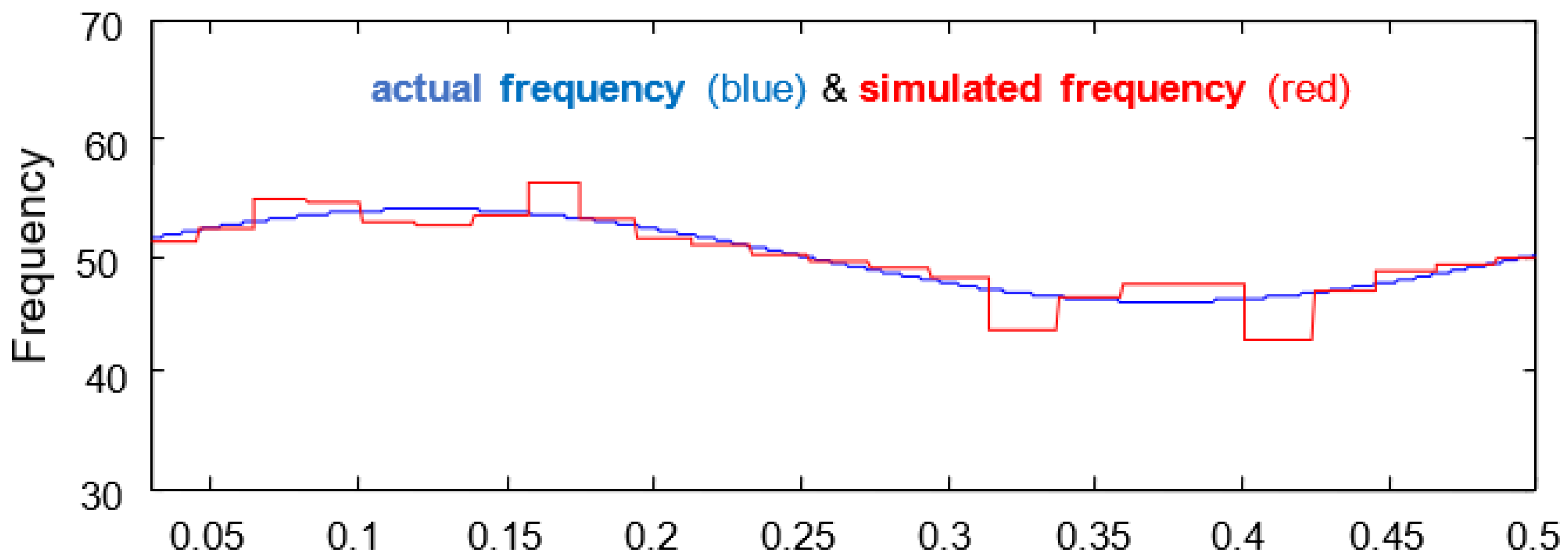
Figure 5 show the frequency of the first harmonic, the blue waveform is the actual frequency of the first harmonic, and the waveform of the frequency calculated by the algebraic method.

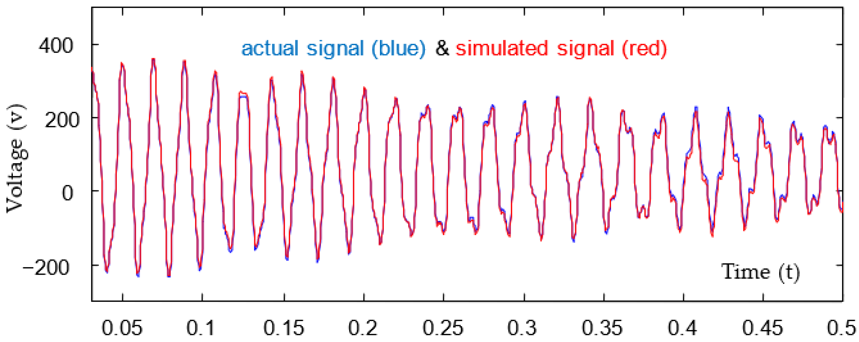
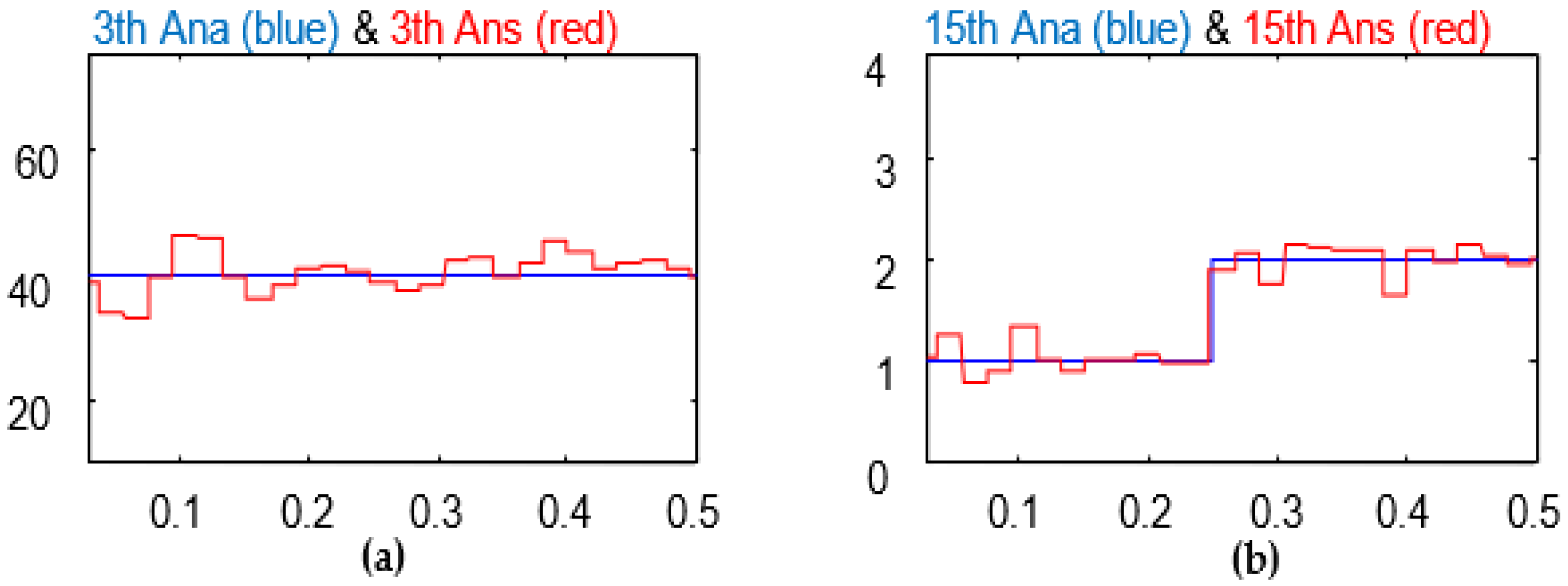
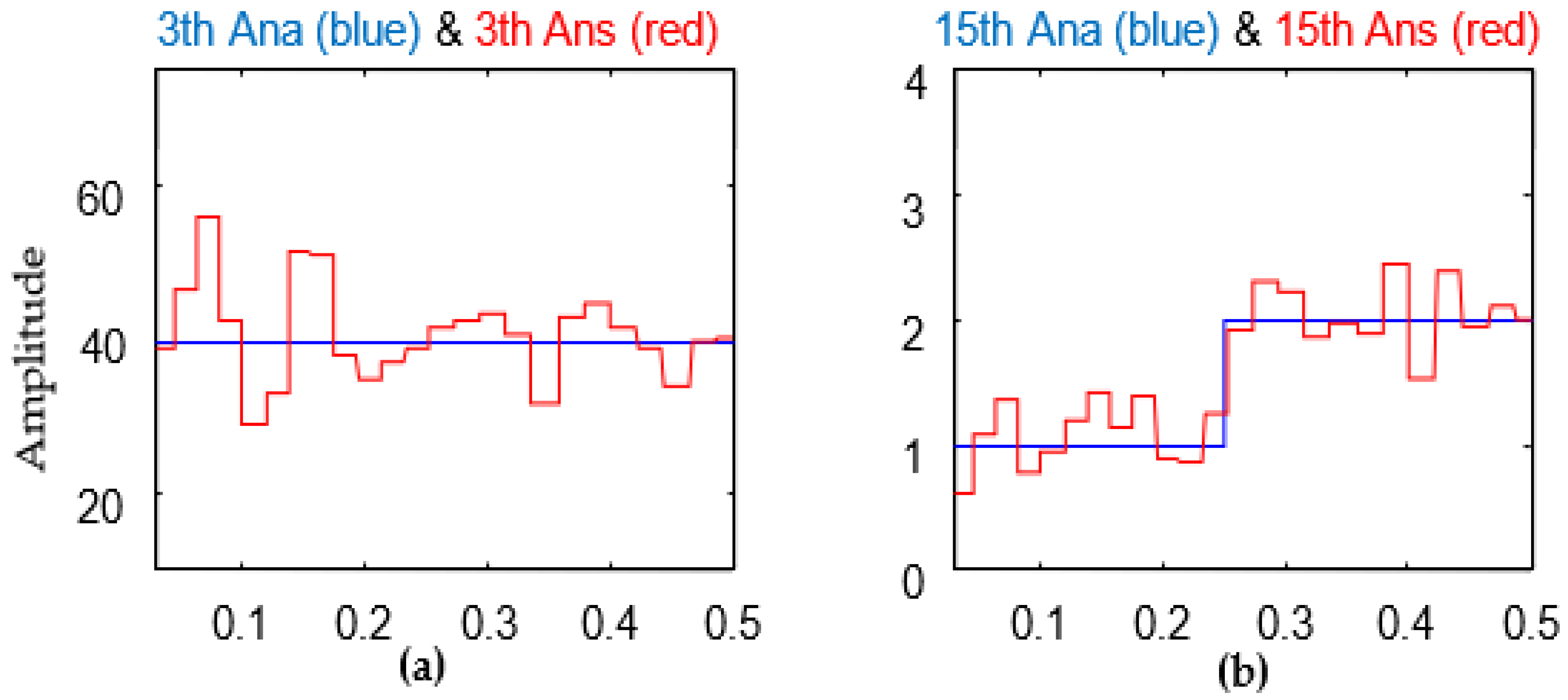
Figure 6 shows the voltage waveform simulated by algebraic method and its actual value. Figure 7a and Figure 7b show the amplitude and phase of the first harmonics, respectively. Figure 8a and Figure 8b also show the range of the third and fifteenth harmonics, respectively. The algorithm of the DFT method for calculating harmonics is shown in Figure 9.

3.1.6. Simulation for DFT Method

In order to demonstrate the capability of the DFT method, the voltage of the power network is considered as follows [37]:

$$v\left(t\right)=v_{DC}+{\displaystyle \sum _{n\hspace{0.17em}\hspace{0.17em}=\hspace{0.17em}\hspace{0.17em}1}^{20}{A}_n\hspace{0.17em}\sin \left(2\pi \hspace{0.17em}nf\hspace{0.17em}t+{\varphi }_{\hspace{0.17em}n}\right)}$$

(34)

where

$$A_n=\{\begin{array}{l}300\hspace{0.17em}{e}^{-\hspace{0.17em}2\hspace{0.17em}t}\hspace{0.17em}\hspace{0.17em},\hspace{0.17em}n=1\\ 40\hspace{0.17em}\hspace{0.17em}\hspace{0.17em}\hspace{0.17em}\hspace{0.17em}\hspace{0.17em}\hspace{0.17em}\hspace{0.17em}\hspace{0.17em},\hspace{0.17em}n=3\\ u\left(t\right)+u\left(t-0.25\right)\hspace{0.17em}\hspace{0.17em}\hspace{0.17em}\hspace{0.17em}\hspace{0.17em}\hspace{0.17em}\hspace{0.17em},\hspace{0.17em}n=15\\ 0\hspace{0.17em}\hspace{0.17em}\hspace{0.17em}\hspace{0.17em}\hspace{0.17em}\hspace{0.17em}\hspace{0.17em}\hspace{0.17em}\hspace{0.17em}\hspace{0.17em},\hspace{0.17em}\hspace{0.17em}Otherwise\hspace{0.17em}\hspace{0.17em}\end{array}\begin{array}{l}{v}_{, DC}=60\hspace{0.17em}\hspace{0.17em}\hspace{0.17em}\hspace{0.17em}\hspace{0.17em}\hspace{0.17em}\hspace{0.17em},\hspace{0.17em}f=50\\ {\varphi }_{\hspace{0.17em}n}=\{\begin{array}{l}-2\hspace{0.17em}\cos \left(2\pi \hspace{0.17em}2\hspace{0.17em}t\right)\hspace{0.17em}\hspace{0.17em}\hspace{0.17em}\hspace{0.17em}\hspace{0.17em}\hspace{0.17em}\hspace{0.17em}\hspace{0.17em},\hspace{0.17em}n=1\\ \\ \hspace{0.17em}0\hspace{0.17em}\hspace{0.17em}\hspace{0.17em}\hspace{0.17em}\hspace{0.17em}\hspace{0.17em}\hspace{0.17em}\hspace{0.17em}\hspace{0.17em}\hspace{0.17em}\hspace{0.17em}\hspace{0.17em}\hspace{0.17em}\hspace{0.17em}\hspace{0.17em}\hspace{0.17em}\hspace{0.17em}\hspace{0.17em}\hspace{0.17em}\hspace{0.17em}\hspace{0.17em}\hspace{0.17em}\hspace{0.17em},\hspace{0.17em}n\ne 1\end{array}\end{array}$$

The variability of the first harmonic phase (fundamental) causes the variability of the first frequency of the signal. In this case, the first harmonic frequency is:

$$f_1=\frac{1}{2\pi }\frac{d}{d\hspace{0.17em}t}\left(2\pi \hspace{0.17em}f\hspace{0.17em}t+\hspace{0.17em}{\varphi }_{\hspace{0.17em}1}\right)=f\hspace{0.17em}+4\hspace{0.17em}\sin \left(2\pi \hspace{0.17em}2\hspace{0.17em}t\right)$$

(35)

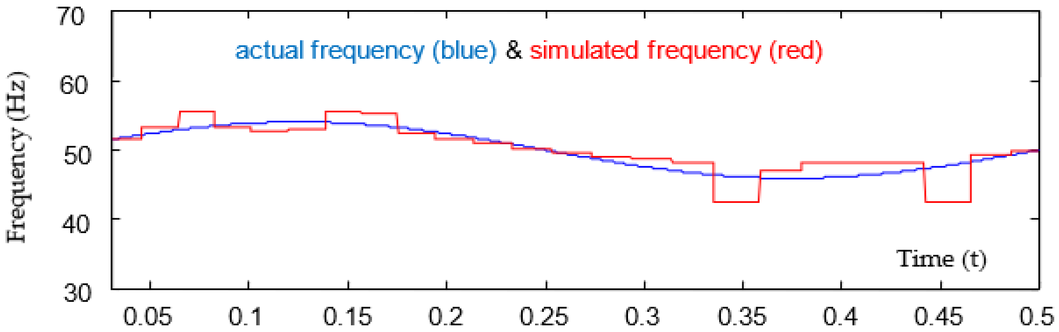
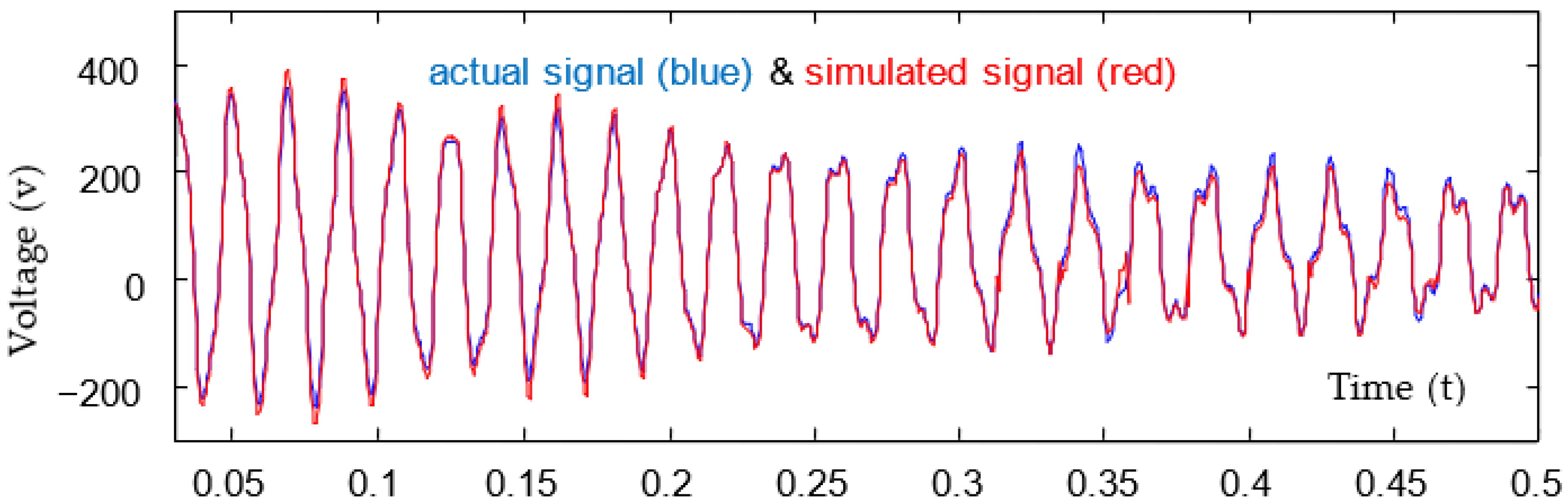
Figure 10 shows the frequency of the first harmonic, the blue waveform is the actual frequency of the first harmonic, and the waveform of the frequency calculated by the DFT method. Figure 11 shows the voltage waveform simulated by DFT method and its actual value. Figure 12a,b show the amplitude and phase of the first harmonics, respectively. Figure 13a,b also show the amplitude of third and fifteenth harmonics, respectively.

One of the drawbacks of the DFT method is the leakage in the spectrum. This effect occurs due to the windowing of the signal under analysis in the time domain and corresponds to the Fourier transform of that window. Figure 14 shows the windowing of the signal in the time domain. As we know, convolutional in the frequency domain means integration over all components of the frequency spectrum. Furthermore, this means the influence of adjacent spectra in the harmonics to be calculated. In other words, spectral energy leaks from one frequency to another due to windowing. The following can be mentioned as ways to reduce this effect: (1) increasing the window’s width by increasing the number of DFT points inside this window; (2) using appropriate window functions; (3) removing large intermittent components before windowing [38].

3.1.7. Comparison of the Algebraic Method with the Dynamic Gradient Method

In the algebraic method, for 2N + 1 samples during a period, N harmonics and the DC value of the waveform can be obtained entirely (analytically). However, this possibility does not exist in the least squares method; in other words, to increase the accuracy in this method, the number of samples should be increased [39]. In terms of speed, it can be seen that if we convert these methods into reversibility, their speeds will ultimately be the same. It should be noted that it is possible to calculate the instantaneous frequency for the least squares method. However, this possibility is not directly possible for the algebraic method [40].

3.2. Compression Monitored Variables

For making offline analysis available, we must be able to store the frequency, $v_{DC}$ magnitude, harmonics (steady values), and transient modes, and for the maximum decreasing of memory values, we must compress them. For this proposal, we present a method for compressing transient values and a new method for compressing steady values [41].

3.2.1. Compression of Transient Modes

Transient modes are characterized by the first level of wavelet factor ($d_1\left(n\right)$). To save this level, we pass it through a limiter. If we show the limiting output in terms of input ($d_1$) as (${\widehat{d}}_1$) (according to Figure 15), then we will have:

$${\widehat{d}}_1\left(n\right)=\{\begin{array}{l}{d}_1\left(n\right)\hspace{0.17em}\hspace{0.17em},\hspace{0.17em}\left|d_1\left(n\right)\right|\ge \eta \\ 0 \hspace{0.17em}\hspace{0.17em}\hspace{0.17em}\hspace{0.17em}\hspace{0.17em}\hspace{0.17em}\hspace{0.17em},\hspace{0.17em}\left|d_1\left(n\right)\right|<\eta \end{array}$$

(36)

Thus when the amount of $d_1$ is smaller than specific values, ${\widehat{d}}_1$ will be zero, and otherwise ${\widehat{d}}_1=d_1$. In this manner, in additionally performed compression, the disturbance of $d_1$, which has a high-frequency spectrum, is also omitted [42].

3.2.2. Compression of DC Value and Amplitude and Phase of Signal Harmonics

DC value, amplitude, and phase of signal harmonics are steady-state parts of the signal, and usually, its changes are smooth and predictable. The consecutive values for these variables are the values obtained for them in their corresponding consecutive periods. Because the changes in these signals are slow, we therefore approximate the signal with a third-degree function. In order for this approximation to be more accurate, the coefficients of this function (third-order function) are recalculated based on the restrictions mentioned later. The least square technique is used to approximate the signal. That technique is also solved via the reversible algebraic method [43].

Assume $a\left(k\right)$ (in Figure 16) is the magnitude of any harmonics that we intend to compact. For this purpose, first, we divide it into different areas. Then, we approximate each of these areas using the third-degree function. To specify these time ranges, we apply the following restrictions [43]. These constraints are considered so that, while minimizing the third-order function with the waveform, the amount of compression is also maximized. It should be noted that the more extensive the selected spatial range, the more significant the amount of compression, which will be discussed in detail in the next section.

The constraints based on which the coefficients of the third-degree function change are as follows:

(a)

One of the other places where the coefficients of the third-order function should change is the place where, firstly, the derivative of the signal changes its sign, and secondly, the absolute value of the difference in the signal value at that place is greater than a particular value, i.e., [44]:

$$\begin{array}{l}\hspace{0.17em}if\hspace{0.17em}\hspace{0.17em}\hspace{0.17em}\dot{a}\left(k\right)=\frac{a\left(k\right)-a\left(k-1\right)}{\Delta k}\hspace{0.17em}\hspace{0.17em}\hspace{0.17em}\\ \hspace{0.17em}then\hspace{0.17em}\hspace{0.17em}\hspace{0.17em}\{\begin{array}{l}1:\hspace{0.17em}\hspace{0.17em}\dot{a}\left(k\right)\cdot \dot{a}\left(k-1\right)<0\\ 2:\hspace{0.17em}a\left(k\right)-a\left(k_m\left(m-1\right)\right)>\eta \end{array}\end{array}$$

(37)

In Equation (37), $m,k_m$ are the number of internal approximations and the end of the previous range, in $m$ intervals, respectively.

(b)

The interval of the period, from the end of previous interval $\left(m-1\right)$, is more significant than another specific amount $L$; namely:

$$l=k-k_m\left(m-1\right)\ge L$$

(38)

3.3. Approximation of the Signal under Compression

As said before, to calculate the coefficients in each period (m = 1000), we try to minimize the square of the error of the third-degree function and the signal under compression. For this purpose, we use an analytical method and make it reversible so that the calculations are divided between the periods. Suppose the signal under compression is a(k) in period m. This signal is approximated by the following third-degree function in the mentioned range [45].

$$p\left(l\right)=a_3\hspace{0.17em}{l}^3+a_2\hspace{0.17em}{l}^2+a_1\hspace{0.17em}l+a_0$$

(39)

In this case, the squared error of the signal under compression and the third-degree function in this range is:

$$E\left(l\right)=a\left(l-km\left(m-1\right)\right)-p\left(l\right)\hspace{0.17em}\hspace{0.17em}\hspace{0.17em}\hspace{0.17em}\Rightarrow \hspace{0.17em}\hspace{0.17em}\hspace{0.17em}\hspace{0.17em}\hspace{0.17em}\hspace{0.17em}\hspace{0.17em}{e}^2={\displaystyle \sum _{l}E\left(l\right)}\hspace{0.17em}$$

(40)

For simplicity, in the following, we consider $a\left(l-km\left(m-1\right)\right)$ to be equal to $y\left(l\right)$. In order for $p\left(l\right)$ to be closer to $a\left(k\right)$, the function $e^2$ should be minimized.

Reversible Algebraic Method

To minimize $e^2$, its derivatives in terms of variables $a_0\hspace{0.17em}\hspace{0.17em},\hspace{0.17em}{a}_1\hspace{0.17em}\hspace{0.17em},\hspace{0.17em}{a}_2\hspace{0.17em}\hspace{0.17em},\hspace{0.17em}{a}_3$ can be set equal to zero. We have in this order [46]:

$$\begin{array}{lll}\frac{\partial \hspace{0.17em}{e}^2}{\partial \hspace{0.17em}{a}_3}=0& \Rightarrow 2\hspace{0.17em}E\hspace{0.17em}{l}^3=0& \Rightarrow a_3\hspace{0.17em}{\displaystyle \sum _l{l}^6}+a_2\hspace{0.17em}{\displaystyle \sum _l{l}^5}+a_1\hspace{0.17em}{\displaystyle \sum _l{l}^4}+a_0\hspace{0.17em}{\displaystyle \sum _l{l}^3}={\displaystyle \sum _{l}y\left(l\right)}\hspace{0.17em}{l}^3\\ \frac{\partial \hspace{0.17em}{e}^2}{\partial \hspace{0.17em}{a}_2}=0& \Rightarrow \hspace{0.17em}\hspace{0.17em}2\hspace{0.17em}E\hspace{0.17em}{l}^2=0& \Rightarrow a_3\hspace{0.17em}{\displaystyle \sum _l{l}^5}+a_2\hspace{0.17em}{\displaystyle \sum _l{l}^4}+a_1\hspace{0.17em}{\displaystyle \sum _l{l}^3}+a_0\hspace{0.17em}{\displaystyle \sum _l{l}^2}={\displaystyle \sum _{l}y\left(l\right)}\hspace{0.17em}{l}^2\\ \frac{\partial \hspace{0.17em}{e}^2}{\partial \hspace{0.17em}{a}_1}=0& \Rightarrow \hspace{0.17em}\hspace{0.17em}2\hspace{0.17em}E\hspace{0.17em}l=0& \Rightarrow a_3\hspace{0.17em}{\displaystyle \sum _l{l}^4}+a_2\hspace{0.17em}{\displaystyle \sum _l{l}^3}+a_1\hspace{0.17em}{\displaystyle \sum _l{l}^2}+a_0\hspace{0.17em}{\displaystyle \sum _{l}l}={\displaystyle \sum _{l}y\left(l\right)}\hspace{0.17em}l\\ \frac{\partial \hspace{0.17em}{e}^2}{\partial \hspace{0.17em}{a}_0}=0& \Rightarrow \hspace{0.17em}\hspace{0.17em}2\hspace{0.17em}E=0& \Rightarrow a_3\hspace{0.17em}{\displaystyle \sum _l{l}^3}+a_2\hspace{0.17em}{\displaystyle \sum _l{l}^2}+a_1\hspace{0.17em}{\displaystyle \sum _{l}l}+a_0\hspace{0.17em}{\displaystyle \sum _{l}1}={\displaystyle \sum _{l}y\left(l\right)}\hspace{0.17em}\end{array}$$

(41)

In this way, the following algebraic equation is obtained from Equation (6).

$$\left[\begin{array}{l}{a}_3\\ a_2\\ a_1\\ a_0\end{array}\right]={\left[\begin{array}{l}{A}_6\hspace{0.17em}\hspace{0.17em}{A}_5\hspace{0.17em}\hspace{0.17em}{A}_4\hspace{0.17em}\hspace{0.17em}{A}_3\\ A_5\hspace{0.17em}\hspace{0.17em}{A}_4\hspace{0.17em}\hspace{0.17em}{A}_3\hspace{0.17em}\hspace{0.17em}{A}_2\\ A_4\hspace{0.17em}\hspace{0.17em}{A}_3\hspace{0.17em}\hspace{0.17em}{A}_2\hspace{0.17em}\hspace{0.17em}{A}_1\\ A_3\hspace{0.17em}\hspace{0.17em}{A}_2\hspace{0.17em}\hspace{0.17em}{A}_1\hspace{0.17em}\hspace{0.17em}{A}_0\end{array}\right]}^{\hspace{0.17em}-1}\hspace{0.17em}\hspace{0.17em}\left[\begin{array}{l}{Y}_3\\ Y_2\\ Y_1\\ Y_0\end{array}\right]\hspace{0.17em}$$

(42)

The values of $A_j$, which is $\left(j=0\hspace{0.17em},\hspace{0.17em}\cdots \hspace{0.17em},\hspace{0.17em}6\right)$, and $Y_i$, which is $\left(i=0\hspace{0.17em},\hspace{0.17em}\cdots \hspace{0.17em},\hspace{0.17em}3\right)$, can be reversibly calculated [47]:

$$\begin{array}{l}{A}_j\left(l\right)=A_j\left(l-1\right)+l^j\\ Y_i\left(l\right)=Y_i\left(l-1\right)+y\left(l\right)\hspace{0.17em}{l}^i\end{array}$$

(43)

Thus, at the end of each range, we have:

$$\begin{array}{l}{A}_j=A_j\left(l\right)\\ Y_i=Y_i\left(l\right)\end{array}$$

(44)

This means that all the matrix elements of coefficients $\left(A_{4\hspace{0.17em}\times 4}\right)$ and vector $Y_{4 \times 1}$ are calculated until the end of each range. 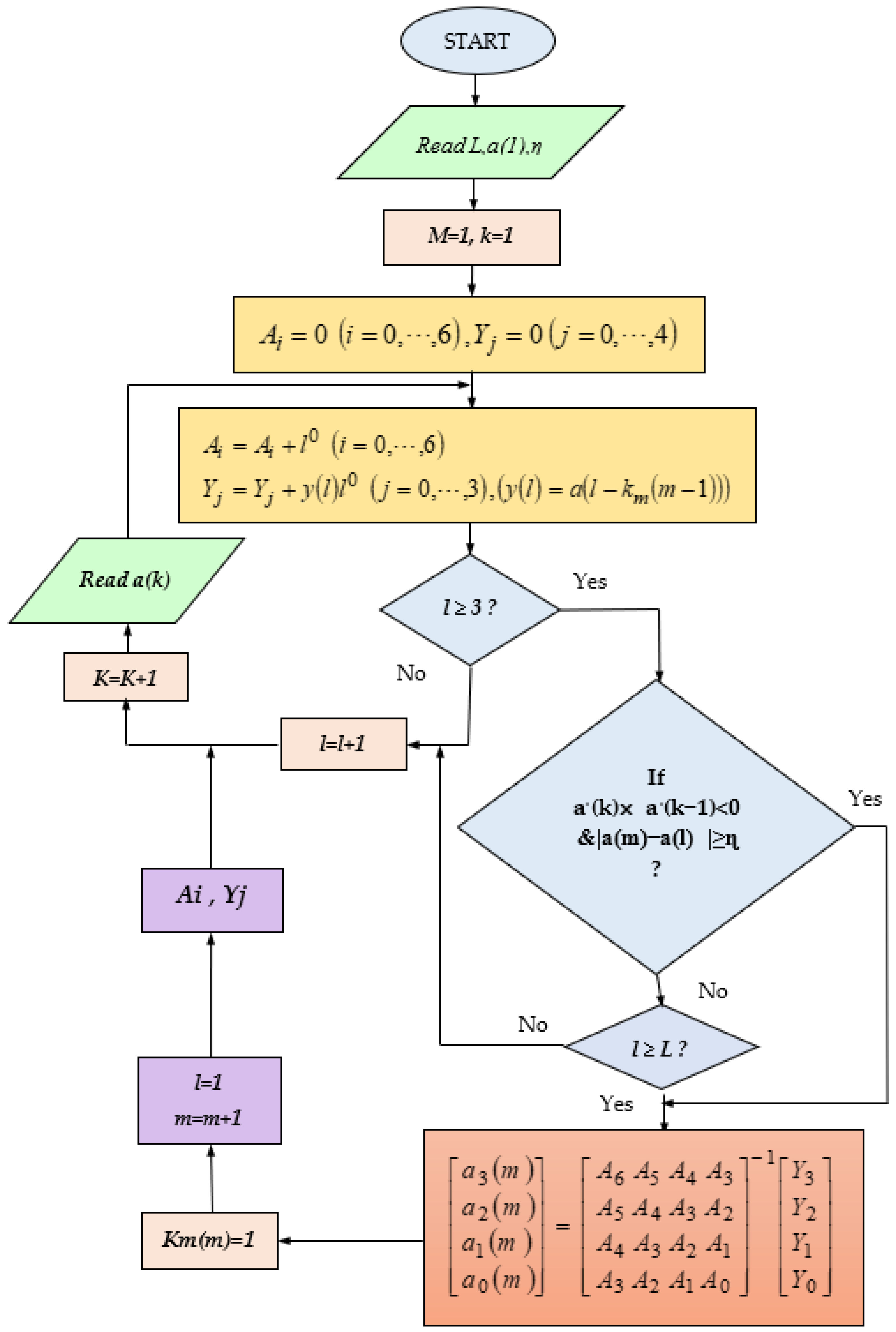Moreover, in the end, it becomes possible to calculate the variables $a_0\hspace{0.17em}\hspace{0.17em},\hspace{0.17em}{a}_1\hspace{0.17em}\hspace{0.17em},\hspace{0.17em}{a}_2\hspace{0.17em}\hspace{0.17em},\hspace{0.17em}{a}_3$ in much less time. In order to better understand the harmonics compression method, the process of compressing the harmonics permanent part is presented as an algorithm. The algorithm of the compression of steady-state harmonics is shown in Figure 17. In this algorithm, $a\left(k\right)$ is simulated by $a_0\left(m\right)+a_1\left(m\right)l+a_2\left(m\right)l^2+a_3\left(m\right)l^3$, and $y$ is $a\left(k-k_m\left(m-1\right)\right)$.

3.4. Amount of Compression

In this part, we want to examine the amount of compression via the mentioned system. The number of samples of the main signal is 24 thousand samples per second. This signal is divided into two parts, one of which represents the transient state (wavelet factor), and the other represents the steady state (scaling factor). Because we have assumed that the frequency spectrum (harmonics order) of the steady state of the power network signal is limited to the 20th harmonic, it is therefore necessary to take 41 × 50 = 2050 samples from the harmonic part of the signal to calculate the harmonics and the DC value. Alternatively, in other words, we use only samples 41 × 50 = 2050 s apart (in this case, the signal frequency is 50 Hz). But after calculating the harmonics, for each period of the signal, 41 values (20 harmonics size values, 20 harmonics phase values, and one for the DC value) are calculated. Therefore, there is no change in the amount of data before and after the harmonics measurement. So far, assuming that the length of transient states that have occurred is 1% on average for each second, then furthermore, the remaining 99% can be considered deleted after passing through the limiter; the number of data have been halved.

However, from the harmonics, the wavelet is taken first. Furthermore, its steady part is passed through the compression system explained in the previous section. If we consider the number of periods in each range to be 50 periods on average, we will have the following: the number of compression values in each range is 5. While the number of data in each limit is considered to be 50, it can be seen that the amount of compression is [48]:

$$\begin{array}{l}COM\stackrel{\Delta }{=}\frac{X_{Actual}}{X_{Compression}}\\ \hspace{0.17em}\hspace{0.17em}\hspace{0.17em}\hspace{0.17em}\hspace{0.17em}\hspace{0.17em}\hspace{0.17em}=\frac{(24000/50) \times 50}{(41 \times 5) + 0.02 \times (12000/50) \times 50}\approx 54\end{array}$$

(45)

where $X_{Actual},\hspace{0.17em}{X}_{Compression}$ are the amount of original signal data in a range and the amount of compressed signal data, respectively.

3.5. Harmonic Recovery

In this part, the values of harmonics are retrieved for different values. After receiving the time when the values of the harmonics are required for that moment, the order of the period in which this time is located is calculated.

$$k=\left[f\times t\right]+1$$

(46)

In the above relation, k is the order of the period, and $\left[f\times t\right]$ is the absolute value of the signal frequency and the time for which the harmonics are to be calculated. Then, the range of compression in which k is located is determined, namely [49]:

$$k_m\left(m-1\right)<k\le k_m\left(m\right)$$

(47)

$$m=1\hspace{0.17em},\hspace{0.17em}\hspace{0.17em}k=\left[f\times t\right]+1$$

(48)

$$l=k-k_m\left(m-1\right)$$

(49)

$$a\left(k\right)=a_0\left(m\right)+a_1\left(m\right)l+a_2\left(m\right)l^2+a_3\left(m\right)l^3$$

(50)

In this relation, $m,\hspace{0.17em}{k}_m$ are the number of the compression interval and the number of the last period that exist this interval, respectively. Harmonics in any interval are specified through calculation of $m,\hspace{0.17em}{k}_m$. The harmonics recovery algorithm is shows in Figure 18.

4. Simulation and Results

4.1. Real-Time and Offline Analysis of Power System

By obtaining the transient states and harmonics of the voltage and current of the power network phases, the quality of the power network can be analyzed, and necessary electrical quantities can be obtained. These quantities are as follows: the practical values of the voltage and currents of the power network, and the real and imaginary components of the apparent power of the network and also positive, negative, and neutral sequences in real time.

4.1.1. Finding the Location of the Fault by Derivation

Occurred faults are of high importance when they have significant effects on the main component of the power grid voltage. In this case, the fault occurrence time can be obtained by deriving the waveform of the main component of the signal. This is because if we represent this time with $t_{fault}$, then the difference between two samples before and after the error will be more significant than the difference between consecutive samples in typical moments. Therefore, the derivative will be significant at this moment. This means that:

$$\dot{x}\left(t_{fault}\right)\approx \frac{x\left(t_{fault}^{+}\right)-x\left(t_{fault}^{-}\right)}{\Delta \hspace{0.17em}t}$$

(51)

In this relation, $t_{fault}^{+}\hspace{0.17em}\hspace{0.17em}\hspace{0.17em},\hspace{0.17em}\hspace{0.17em}{t}_{fault}^{-}$ are, respectively, the sampling times before and after the occurrence of the fault.

However, the derivative of the sinusoidal signal (the main component of the voltage waveform) cannot always be determined when the fault occurs.

In Figure 19, the derivative of the signal at the fault location does not differ much from the derivative of the signal at ordinary moments. Therefore, the derivative of the signal cannot determine the occurrence of the fault.

However, in Figure 20, the derivative of the signal at the moment of the fault is significantly different from the derivative of the signal at normal moments. So, it is possible to determine the occurrence of the fault from the derivative of the signal.

It can be seen from the above figure that it is possible to determine the half period of the signal in which the fault occurred. In other words, this time is enclosed between two times in which the signal has the maximum value before the fault and the minimum value after the fault or vice versa (minimum before the fault and maximum after the fault).

It can be seen that in Figure 21, the fault occurred when the value of the sine function is close to zero. Therefore, the derivative of the function will be insignificant at this point.

However, in Figure 22, a fault has occurred in a place where the value of the sinusoidal function is close to one, regardless of its sign. Therefore, the value of the derivative of the signal at this moment is substantial.

4.1.2. Accurate Determination of the Fault Occurrence Time Using Wavelet Transform

As was said before, the first wavelet level of any signal can show the location of the fault in time and frequency.

After taking the wavelet transform (as shown in Figure 23), the wavelet coefficient represents the transient modes. Next, for Figure 24 and Figure 25, the wavelet coefficient and scale coefficient are shown.

For this case, it was observed that we could not obtain the location of the change in the monitored signal through derivation. Nevertheless, in part (c) of the above figure, it can be seen that the location of the change in the signal under study can be easily found. This part actually shows the waveform of wavelet’s factor.

4.2. Offline Analysis of the Power Network

Considering that the provided monitoring system is able to store harmonics and transient states, they can therefore be used for offline analysis such as statistical harmonics analysis.

4.3. Simulation of Compression Steady Values

Normally, the waveform of the harmonics and DC value is sinuous or exponential. Thus, we use the presented algorithm for steady compression over these waveforms.

(a)

Exponential waveform: If $a\left(k\right)$ is considered as follows:

$$a\left(k\right)=200e^{-0.02\hspace{0.17em}k}$$

(52)

then for $k=1,\cdots ,100$, we can show $a\left(k\right)$, and the simulation is as shown in Figure 26.

(b)

Sinuous waveform: If $a\left(k\right)$ is considered as follows:

$$a\left(k\right)=\sin \left(0.02\pi \hspace{0.17em}k\right)$$

(53)

then for $k=1,\cdots ,100$, we can show $a\left(k\right)$, and the simulation is as shown in Figure 27.

5. Comparison Results with Other Papers

In order to check the quality of the proposed method, a comparison has been made between the results of this study and the results of the articles in

Table 1. The accuracy results of the proposed method in the classification of power quality disturbances in comparison with previous articles.

Some of the Power Quality Studies		Number of Features	Classification Accuracy (%)
References			Noiseless	40 dB	30 dB	20 dB	Overall
[5]		7	99.65	99.4	99.2	87	96.62
[8]		17	99.78	--	99.41	97.79	97.93
[11]		8	99.76	99.57	96.98	84.86	96.22
[13]		5	--	99.46	99.11	94	98.08
[18]		12	99.88	94.64	93.85	89.92	91.8
[32]		14	--	92.64	--	93.19	94.16
[38]		16	99.55	99.54	99.21	94.91	98.31
This paper	Online Scheme	6	99.66	99.33	99.33	98.77	99.38
	Offline Scheme	6	99.77	99.44	99.66	99.44	99.66

in terms of the percentage of classification accuracy and the dimensions of the feature vector. This comparison shows that the classification algorithms presented in this research have high immunity despite the high noise. Also, the overall accuracy in this research is higher than all the mentioned articles. Therefore, the proposed detection structures perform best in noisy conditions without using denoising algorithms, and power quality disturbances can be detected without the complexity of performing noise steps and calculations with an appropriate accuracy.

It should be noted that for the better understanding of the readers and to help the related research in the future, parts of the written computer program are given in Appendix A.

6. Conclusions

In recent times, the non-linear loads in power networks have increased, so the identification of harmonics is critical. Because of this, in order to analyze the network with such loads, the number of harmonics must be known. One of the important parameters in controlling and studying the stability of power systems is the power grid frequency. Therefore, it is necessary to determine its momentary changes; in other words, it should be possible to measure it momentarily.

In this paper, we present a monitoring system that is able to calculate frequency, harmonics, and DC value and transient events. In this research, different methods of frequency and harmonics have been presented and compared to each other. DFT method, algebraic method, and least square method are the three main methods of calculating harmonics and calculating frequency. Techniques to improve these methods have been provided. Based on the comparison, the reversible algebraic method is superior to the others, while being simpler to implement, with high accuracy and speed. Therefore, this method has been used in the monitoring system.

In order to diagnose faults and study their effects on a power network, transient states must be identified. For this purpose, the mathematical technique of signal processing called wavelet transform is used today. We have also used this method to identify the faults that occurred in a power network. In addition to displaying signals in time and frequency domains, a wavelet can display them with the least coefficients. This is because their coefficients rapidly tend to zero with an increase in their levels if the mother wavelet function is selected.

The provided monitoring system provides harmonics and transients for real-time and offline analysis. To perform offline analysis, the measured values must be stored. Obviously, if these measured data are stored directly, they will occupy a significant amount of memory. To reduce the memory usage, it is necessary to compress the measured values before being stored. The provided monitoring system can multiply the data obtained from the measurement by a new and unique method up to 40 times (while maintaining maximum accuracy).

The simulation results obtained in this article show that this structure and approach are superior to other approaches used in recent years in the discussion of monitoring power quality disturbances.

Due to the introduction of a new processing technique (wavelet transform), which is used to analyze transient states from different points of view that were briefly mentioned, the suggestion that can be made here is to study and complete each of these methods. In particular, these items include the following:

-

Studying and improving the exact location of the fault between two parts of the power network, in which it is possible to accurately measure the quantities of the power network (voltage and current).

-

Finding the most suitable mother wavelet function, which has maximum compatibility with power network signals.

-

The development of methods for finding high-impedance faults by wavelet transform.

-

The development and improvement of detecting the location of the short circuit fault and identifying its type with the help of wavelet transform.

-

Studying the effects of lightning on the transmission system and power distribution system and their equipment.

-

Improving compression methods and the provided monitoring system.

-

The use of neural and fuzzy networks and a genetic algorithm in different parts of the techniques used in the monitoring system.

References

- Rao, S.N.V.B.; Kumar, Y.V.P.; Pradeep, D.J.; Reddy, C.P.; Flah, A.; Kraiem, H.; Al-Asad, J.F. Power quality improvement in renewable-energy-based microgrid clusters using fuzzy space vector PWM controlled inverter. Sustainability 2022, 14, 4663. [Google Scholar] [CrossRef]
- Eslami, A.; Negnevitskyet, M.; Franklin, E.; Lyden, S. Review of AI applications in harmonic analysis in power systems. Renew. Sustain. Energy Rev. 2022, 154, 111897. [Google Scholar] [CrossRef]
- Zhang, Y.; Shi, X.; Zhang, H.; Cao, Y.; Terzija, V. Review on deep learning applications in frequency analysis and control of modern power system. Int. J. Electr. Power Energy Syst. 2022, 136, 107744. [Google Scholar] [CrossRef]
- Rahiman, Z.; Dhandapani, L.; Natarajan, R.C.; Vallikannan, P.; Palanisamy, S.; Chenniappan, S. Power Quality Conditioners in Smart Power System. In Artificial Intelligence-Based Smart Power Systems; Wiley-IEEE Press: Hoboken, NJ, USA, 2023; pp. 233–258. [Google Scholar]
- Sivaraman, P.; Sharmeela, C.; Balaji, S.; Sanjeevikumar, P.; Elango, S. Power Quality Monitoring of Low Voltage Distribution System Toward Smart Distribution Grid Through IoT. In IoT, Machine Learning and Blockchain Technologies for Renewable Energy and Modern Hybrid Power Systems; River Publishers: Abingdon, UK, 2023; pp. 61–77. [Google Scholar]
- Begovic, M.M.; Djuric, P.M.; Dunlap, S.; Phadke, A.G. Frequency Traking in Power Networks in the Presence of Harmonics. IEEE Trans. Power Deliv. 1993, 8, 480–486. [Google Scholar] [CrossRef]
- Phadke, A.G.; Thorp, J.S.; Adamiak, M.G. A New Measurement for Technique Voltage Phasores, Local System Frequency, and Rate of Change of Frequency. IEEE Trans. Power Appar. Syst. 1983, PAS-102, 1025–1038. [Google Scholar] [CrossRef]
- George, T.A.; Bone, D. Harmonic Power Flow Determination Using the FFT transform. IEEE Trans. Power Deliv. 1991, 6, 530–535. [Google Scholar] [CrossRef]
- Narasimhulu, N.; Awasthy, M.; de Prado, R.P.; Divakarachari, P.B.; Himabindu, N. Analysis and Impacts of Grid Integrated Photo-Voltaic and Electric Vehicle on Power Quality Issues. Energies 2023, 16, 714. [Google Scholar] [CrossRef]
- Heydet, G.T.; Galli, A.W. Transient Power Quality Analyzed Using wavelets. IEEE Trans. Power Deliv. 1997, 12, 908–915. [Google Scholar] [CrossRef]
- Eristi, H.; Demir, Y. A new algorithm for automatic classification of power quality events based on wavelet transform and SVM. Expert Syst. Appl. 2010, 37, 4094–4102. [Google Scholar] [CrossRef]
- Liang, K.; Xiao, H.; Du, Y.; Lu, C.; Shen, M. A real-time monitoring system for fruit and vegetable cold chain logistics based on Internet of things technology. Jiangsu J. Agric. Sci. 2018, 43, 519–521. [Google Scholar]
- Nanda, P.; Panigrahi, C.K.; Dasgupta, A. Phasor estimation and modelling techniques of PMU-a review. Energy Procedia 2017, 109, 64–77. [Google Scholar] [CrossRef]
- Xu, S.; Leng, X. Design of Real-Time Power Quality Monitoring System for Active Distribution Network Based on Computer Monitoring. J. Phys. Conf. Ser. 2021, 1992, 032127. [Google Scholar] [CrossRef]
- Banuelos-Cabral, E.S.; Nuno-Ayón, J.J.; Sotelo-Castanon, J.; Naredo, J.L. Extended vector fitting for subharmonics, harmonics, interharmonics, and supraharmonics estimation in electrical systems. Electr. Power Syst. Res. 2023, 224, 109664. [Google Scholar] [CrossRef]
- Kirikkaleli, D.; Adebayo, T.S. Do public-private partnerships in energy and renewable energy consumption matter for consumption-based carbon dioxide emissions in India? Environ. Sci. Pollut. Res. 2021, 28, 30139–30152. [Google Scholar] [CrossRef] [PubMed]
- Heydt, G.T.; Fjeld, P.S.; Liu, C.C.; Pierce, D.; Tu, L.; Hensley, G. Application of the Windowed FFT to Electrical Power Quality Assessment. IEEE Trans. Power Deliv. 1999, 144, 1411–1416. [Google Scholar] [CrossRef]
- Mallala, B.; Venkata, P.V.; Palle, K. Analysis of Power Quality Issues and Mitigation Techniques Using HACO Algorithm. In International Conference on Intelligent Sustainable Systems; Springer Nature: Singapore, 2023. [Google Scholar] [CrossRef]
- Zadehbagheri, M.; Payedar, A. The feasibility study of using space vector modulation inverters in two-level of integrated photovoltaic system. TELKOMNIKA Indones. J. Electr. Eng. 2015, 14, 205–214. [Google Scholar] [CrossRef]
- Huang, S.-J.; Hsieh, C.-T. High-Impedance Fault detection Utilizing a Morlet Wavelet Transform Approach. IEEE Trans. Power Deliv. 1999, 14, 1401–1410. [Google Scholar] [CrossRef]
- Zheng, T.; Makram, E.B.; Girgis, A.A. Power System Transient and Hormonic Studies Using Transform. IEEE Trans. Power Deliv. 1999, 9, 1461–1468. [Google Scholar] [CrossRef]
- Balasubbareddy, M.; Venkata Prasad, P.; Palle, K. Power Quality Conditioner with Fuzzy Logic Controller. In Information and Communication Technology for Competitive Strategies (ICTCS 2022); Kaiser, M.S., Xie, J., Rathore, V.S., Eds.; Lecture Notes in Networks and Systems; Springer: Singapore, 2023; Volume 615. [Google Scholar] [CrossRef]
- Abbasi, A.R. Fault detection and diagnosis in power transformers: A comprehensive review and classification of publications and methods. Electr. Power Syst. Res. 2022, 209, 107990. [Google Scholar] [CrossRef]
- Karami, M.; Zadehbagheri, M.; Kiani, M.J.; Nejatian, S. Retailer energy management of electric energy by combining demand response and hydrogen storage systems, renewable sources and electric vehicles. Int. J. Hydrogen Energy 2023, 48, 18775–18794. [Google Scholar] [CrossRef]
- Zahedi, A. A review of drivers, benefits, and challenges in integrating renewable energy sources into electricity grid. Renew. Sustain. Energy Rev. 2011, 15, 4775–4779. [Google Scholar] [CrossRef]
- Gayatri, M.T.L.; Parimi, A.M.; Kumar, A.V.P. Utilization of Unified Power Quality Conditioner for Voltage Sag/Swell Mitigation in Microgrid. In Proceedings of the 2016 Biennial International Conference on Power and Energy Systems: Towards Sustainable Energy (PESTSE), Bengaluru, India, 21–23 January 2016. [Google Scholar]
- Chavhan, S.T.; Bhattar, C.; Koli, P.V.; Rathod, V.S. Application of STATCOM for power quality improvement of grid integrated wind mill. In Proceedings of the International Conference on (ISCO) Intelligent Systems and Control, Coimbatore, India, 9–10 January 2015. [Google Scholar]
- Wang, L.; Vo, Q.-S.; Prokhorov, A.V. Stability improvement of a multimachine power system connected with a large-scale hybrid windphotovoltaic farm using a supercapacitor. IEEE Trans. Ind. Appl. 2018, 54, 50–60. [Google Scholar] [CrossRef]
- Ashraf, N.; Abbas, G.; Ullah, N.; Al-Ahmadi, A.A.; Raza, A.; Farooq, U.; Jamil, M. Investigation of the Power Quality Concerns of Input Current in SinglePhase Frequency Step-Down Converter. Appl. Sci. 2022, 12, 3663. [Google Scholar] [CrossRef]
- Ravi, T.; Kumar, K.S. Analysis, monitoring, and mitigation of power quality disturbances in a distributed generation system. Front. Energy Res. 2022, 10, 989474. [Google Scholar] [CrossRef]
- Zadehbagheri, M.; Ildarabadi, R.; Nejad, M.B.; Sutikno, T. A new structure of dynamic voltage restorer based on asymmetrical γ-source inverters to compensate voltage disturbances in power distribution networks. Int. J. Power Electron. Drive Systems 2017, 8, 344–359. [Google Scholar] [CrossRef]
- Daneshfar, F.; Bevrani, H. Load– frequency control: A GA-based multiagent reinforcement learning. IET Gener. Transm. Distrib. 2010, 4, 13–26. [Google Scholar] [CrossRef]
- Al-Sharafi, A.; Sahin, A.Z.; Ayar, T.; Yilbas, B.S. Techno-economic analysis and optimization of solar and wind energy systems for power generation and hydrogen production in Saudi Arabia. Renew. Sustain. Energy Rev. 2017, 69, 33–49. [Google Scholar] [CrossRef]
- Zheng, J.; Engelhard, M.H.; Mei, D.; Jiao, S.; Polzin, B.J.; Zhang, J.-G.; Xu, W. Electrolyte additive enabled fast charging and stable cycling lithium metal batteries. Nat. Energy 2017, 2, 17012. [Google Scholar] [CrossRef]
- Hemmati, M.; Mirzaei, M.A.; Abapour, M.; Zare, K.; Mohammadi-ivatloo, B.; Mehrjerdi, H.; Marzband, M. Economic-environmental analysis of combined heat and power-based reconfigurable microgrid integrated with multiple energy storage and demand response program. Sustain. Cities Soc. 2021, 69, 102790. [Google Scholar] [CrossRef]
- Posada, J.O.G.; Rennie, A.J.R.; Villar, S.P.; Martins, V.L.; Marinaccio, J.; Barnes, A.; Glover, C.F.; Worsley, D.A.; Hall, P.J. Aqueous batteries as grid scale energy storage solutions. Renew. Sustain. Energy Rev. 2017, 68, 1174–1182. [Google Scholar] [CrossRef]
- Pena-Alzola, R.; Sebastian, R.; Quesada, J.; Colmenar, A. Review of flywheel based energy storage systems. In Proceedings of the 2011 International Conference on Power Engineering, Energy and Electrical Drives, Malaga, Spain, 11–13 May 2011. [Google Scholar]
- Wu, H.; Sun, K.; Li, Y.; Xing, Y. Fixed-Frequency PWM-Controlled Bidirectional Current-Fed Soft-Switching Series-Resonant Converter for Energy Storage Applications. IEEE Trans. Ind. Electron. 2017, 64, 6190–6201. [Google Scholar] [CrossRef]
- Burrus, C.S.; Ramesh; Gopinath, A.; Guo, H. Introduction to Wavelet and Wavelet Transforms; Printice Hall: Upper Saddle River, NJ, USA, 1998. [Google Scholar]
- Li, Y.; Wang, C.; Li, G.; Wang, J.; Zhao, D.; Chen, C. Improving operational flexibility of integrated energy system with uncertain renewable generations considering thermal inertia of buildings. Energy Convers. Manag. 2020, 207, 112526. [Google Scholar] [CrossRef]
- Guo, Y.; Yang, Z.; Feng, S.; Hu, J. Complex power system status monitoring and evaluation using big data platform and machine learning algorithms: A review and a case study. Complexity 2018, 2018, 8496187. [Google Scholar] [CrossRef]
- Al-Khasawneh, M.A.; Bukhari, A.; Khasawneh, A.M. Effective of Smart Mathematical Model by Machine Learning Classifier on Big Data in Healthcare Fast Response. Comput. Math. Methods Med. 2022, 2022, 6927170. [Google Scholar] [CrossRef] [PubMed]
- Uyar, M.; Yildirim, S.; Gencoglu, M.T. An effective wavelet-based feature extraction method for classification of power quality disturbance signals. Electr. Power Syst. Res. 2008, 78, 1747–1755. [Google Scholar] [CrossRef]
- Rodríguez, A.; Aguado, J.A.; Martín, F.; Lopez, J.J.; Munoz, F.; Ruiz, J.E. Rule-based classification of power quality disturbances using S-transform. Electr. Power Syst. Res. 2012, 86, 113–121. [Google Scholar] [CrossRef]
- Olabi, A.G.; Onumaegbu, C.; Wilberforce, T.; Ramadan, M.; Abdelkareem, M.A.; Al-Alami, A.H. Critical review of energy storage systems. Energy 2021, 214, 118987. [Google Scholar] [CrossRef]
- Wei, P.; Abid, M.; Adun, H.; Awoh, D.K.; Cai, D.; Zaini, J.H.; Bamisile, O. Progress in Energy Storage Technologies and Methods for Renewable Energy Systems Application. Appl. Sci. 2023, 13, 5626. [Google Scholar] [CrossRef]
- Kanakadhurga, D.; Prabaharan, N. Demand side management in microgrid: A critical review of key issues and recent trends. Renew. Sustain. Energy Rev. 2022, 156, 111915. [Google Scholar] [CrossRef]
- Mathiesen, B.V.; Lund, H.; Connolly, D.; Wenzel, H.; Østergaard, P.A.; Möller, B.; Nielsen, S.; Ridjan, I.; Karnøe, P.; Sperling, K.; et al. Smart Energy Systems for coherent 100% renewable energy and transport solutions. Appl. Energy 2015, 145, 139–154. [Google Scholar] [CrossRef]
- Barthelemy, H.; Weber, M.; Barbier, F. Hydrogen storage: Recent improvements and industrial perspectives. Int. J. Hydrogen Energy 2017, 42, 7254–7262. [Google Scholar] [CrossRef]
Figure 1.
System voltage waveform.
Figure 2.
Monitoring system: (a) simplified block diagram; (b) simulated structure.
Figure 3.
Voltage signal, scaling factor, and wavelet factor for voltage signal.
Figure 4.
Algorithm of the algebraic method.
Figure 5.
Simulation of the first harmonic frequency (actual and simulated signals).
Figure 6.
Simulation of voltage V(t) (algebraic method).
Figure 7.
(a) First harmonic amplitude; (b) first harmonic phase in rad/(blue curves are actual, and red curves are simulated).
Figure 8.
(a) 3rd harmonic amplitude; (b) 15th harmonic amplitude (blue curves are actual, and red curves are simulated) (algebraic method).
Figure 9.
Algorithm of DFT method for calculating harmonics.
Figure 10.
Simulation of the frequency of the first harmonic (DFT Method).
Figure 11.
The actual value (blue) and the simulated value (red) of the voltage waveform.
Figure 12.
(a) Amplitude of the first harmonic (b) Phase of the first harmonic in terms of radians (the blue curves are actual, and the red curves are simulated).
Figure 13.
(a) 3rd harmonic amplitude; (b) 15th harmonic amplitude (blue curves are actual, and red curves are simulated).
Figure 14.
Windowing of by in the time.
Figure 15.
Limiter for wavelet factor ().
Figure 16.
Waveform under compressing.
Figure 17.
Algorithm of recursive algebraic method for steady-state approximation.
Figure 18.
Harmonics recovery algorithm.
Figure 19.
The waveform of the signal when the fault.
Figure 20.
The waveform of the signal when the fault occurs.
Figure 21.
The fault occurred when the size of the derivative of the signal is minimum at that moment. (a) The signal itself; (b) the derivative of the signal.
Figure 22.
The fault occurred when the size of the derivative of the signal at that moment is maximum. (a) The signal itself; (b) the derivative of the signal.
Figure 23.
Wavelet transform of the signal under analysis.
Figure 24.
The fault occurred when the size of the derivative of the signal is minimum at that moment. (a) Signal itself; (b) scaling factor; (c) wavelet factor.
Figure 25.
The fault occurred when the size of the derivative of the signal is maximum at that moment. (a) Signal itself; (b) scaling factor; (c) wavelet factor.
Figure 26.
(a) Actual and simulated signals. (b) Absolute error between actual and simulated signals.
Figure 27.