Evaluation of Fracture Volume and Complexity of Tight Oil Wells Based on Flowback Data

Abstract

For tight reservoirs, horizontal wells and multi-stage fracturing can generate a complex fracture network that realizes economic and effective development. The volume and complexity of the fracture network are of great significance to accurately predicting the productivity of tight oil wells. In this work, a mathematical model of a multiphase flow is proposed to evaluate the stimulation effect based on the early flowback data. The model showing the early slope of the material balance time (MBT) and production balance pressure (RNP) can help estimate the effective stimulated volume of the horizontal well. The linear flow region can be determined from the slope of the log–log plot of the MBT versus RNP curve, which equals 1. The method is verified by commercial simulation software, and the calculated stimulated volume is consistent with the statistical results of simulation results. Results also show that the flow pattern of the fracture–matrix system can be judged by the slope of the flowback characteristic curve in the early stage of flowback, and then the complexity of the fracture network can also be obtained. The proposed method can provide an avenue to evaluate the fracturing work using the flowback data quickly.

1. Introduction

After the hydraulic fracturing of horizontal wells, the fracturing fluid flows back before production starts. It is generally believed that the retention of fracturing fluid in the formation will cause damage that reduces the formation’s permeability. However, if the flowback is too rapid after fracturing, proppants can flow back and this causes the closure of the generated fracture network, which in turn reduces the well’s productivity.

Currently, the total flowback rate of fracturing fluid in a tight oil reservoir in the Mahu reservoirs is around 10–80% in the first year. It is generally believed that there are two directions for the imbibed fracturing fluid; it can be trapped in smaller pores due to the capillary force or in closed natural or hydraulic fractures. Considering that the flowback fluid fills the main and secondary fractures during hydraulic fracturing, information on the generated fracture network is likely to be contained in the flowback data.

Numerical simulation methods for hydraulic fracturing have been continuously studied with the development of unconventional reservoirs. The calculation models have developed from the initial two-dimensional KGD model and PKN model to a quasi-three-dimensional model that combines KGD and PKN models while including the fracture toughness and leak-off of the fracturing fluid [1]. Models have further developed into full three-dimensional models that consider more realistic formation conditions [2]. The calculation models for hydraulic fractures have been continuously optimized, and the accuracy of the models has been continuously improved.

Several methods are commonly used for simulating hydraulic fractures, including the extended finite element method (XFEM), boundary element method (BEM), and discrete element method (DEM). Each of these calculation methods has its own advantages and disadvantages. Wang et al. investigated the numerical method and equivalent continuum approach (ECA) of fluid flow in the fractured porous media. The commonly used discrete fracture model (DFM) without upscaling needs full discretization of all fractures. It can capture each fracture accurately but will get in trouble with mesh partition and low computational efficiency, especially when a complex geometry is involved [3]. In addition, Wang et al. presented a numerical investigation of fluid flow in the heterogeneous porous media with a consideration of the flux connection of the fracture–cavity network. A hybrid-dimensional modeling approach combined with the dual fracture-pore model is presented [4]. The UFM simulation based on the boundary element method uses a fully coupled numerical method to solve the problem, which fully considers the heterogeneity of the reservoir, the anisotropy of stress, and the stress shadow effect, and can simulate complex fracture network shapes [5]. Not only can it simulate the mechanism of fracture propagation and proppant transport, but it can also effectively simulate the interaction between hydraulic fractures and natural fractures [6].

Scholars have conducted extensive studies on the issue of trapped hydraulic fracturing fluid. The fracturing fluid is distributed in the three-dimensional space surrounding the fractures, including the upper and lower reservoirs of the fractures and the reservoir spaces parallel to the fractures; due to the influence of gravity, the amount of fracturing fluid distributed below the fractures is greater than that above [7]. These can affect the material balance when estimating the volume of the generated fracture network. Furthermore, the reservoir may contain many natural fractures. These geological weak planes have significant differences in mechanical properties and matrix, and during hydraulic fracturing, the hydraulic fractures intersect with the natural fractures in a complex manner. Pagels et al. developed the retention area of the fracturing fluid and found that fracturing fluid would be retained in the natural fracture space that is not connected to the main fractures, as well as in the micro-pores of the formation that are penetrated by imbibition [8]. Cheng et al. found that as the capillary force increases, the amount of imbibition in the rock matrix and natural fractures increases [9]. The wider the natural fractures are, the more fracturing fluid is trapped inside; McClure et al. used numerical simulation to show that the stress field near the intersection of hydraulic fractures and natural fractures can cause fracture closure during fluid flowback, which trapped the fracturing fluid therein [10]. In addition to these disconnected spaces, the reservoir below the fractures affected by gravity may be another main space for fracturing fluid retention; Agrawal et al. used numerical simulation to prove that gravity has a significant impact on the flowback of fracturing fluid [7]; Parmar et al. established the effects of surface tension, gravity, and wettability on the flowback rate of fracturing fluid and found that gravity is the primary influencing factor for the retention of fracturing fluid [11].

Besides the influence of natural fractures and formation properties, researchers have found that the properties of hydraulic fractures themselves can also affect the flowback pattern of the fracturing fluid. Liu et al. found that the tortuosity of complex fractures can affect fluid flowback, mainly because the higher the tortuosity of the fracture is, the weaker is the effect of gravity and the stronger is the capillary imbibition into the rock matrix [12]. Water can invade the matrix adjacent to the complex fracture network, which is unable to flow back [13]. Song et al. found that the diversion ability of hydraulic fractures is the main factor affecting the flowback rate of the fracturing fluid; the poorer the fracture conductivity ability, the lower the flowback rate [14]. Warpinski et al. found that increasing the choke size can improve the flowback rate and enhance production [15]; they also found that the more complex the network of hydraulic fractures is, the higher the corresponding flowback rate is, and thus the complexity of the network of hydraulic fractures can be estimated based on the flowback rate of the fracturing fluid. Modeland et al. found that relatively soft reservoirs may cause proppant embedment, leading to a decrease in fracture conductivity ability and consequently affecting the flowback pattern of the fracturing fluid flowback [16]. Mayerhofer et al. analyzed microseismic data and found that complex fracture networks tend to form in shale reservoirs after hydraulic fracturing [17]. McClure et al. found that the connectivity of complex fracture networks can be reduced due to fracture closure, and therefore, the more complex the fracture network is, the lower the flowback rate is [18]. In addition, Yang et al. believed that the structure and connectivity of complex fracture networks also affect the flowback of fracturing fluid [19].

Together with the rapid development of unconventional reservoirs, researchers have proposed different analysis methods to evaluate the productivity of the horizontal well after hydraulic fracturing. Lee et al. established a trilinear flow model from the conventional bilinear flow model from the matrix through the hydraulic fracture and to the wellbore, and further used this model to study the influence of different fracture parameters on flowback and production curves [20]. Daviau et al. believed that pressure interference exists between fractures due to different fracturing times of multistage fractured horizontal wells, and that it is necessary to calculate multistage fractures separately and then add the inter-fracture interference [21]. Larsen et al. analyzed the flow stages of horizontal wells after hydraulic fracturing and divided them into four stages as follows; linear flow in the fracture, radial flow in the fracture, linear flow in the formation, and pseudo-radial flow [22]. Ozkan et al. optimized the theoretical model based on Lee’s trilinear flow model and analyzed its dynamic characteristics of pressure and productivity based on the solution results [23]. E. Stagorova et al. considered the significant difference in permeability between the formation near the fracture and the distant area and drew typical well-testing curves to analyze the production decline of a well [24].

In general, the flow process of fracturing fluid during flowback can be roughly divided into three stages. In the first stage, the flowing fluid in the fracture is a single-phase fracturing fluid, the pressure in the fracture is high, and the permeability of the fracture is much higher than that of the matrix. After production starts, the matrix flow can be ignored, and the flow in the fracture is considered to be linear. This stage lasts for a short time. In the second stage, the fracture system gradually depressurizes, and due to differences in fracture length and permeability, some fracturing fluids in certain fractures may still be in the linear flow stage, while other fractures may have completely back-flowed. This stage is a transitional period. In the third stage, the pressure in all fractures has propagated to the effective fracture boundary, and the entire fracture system appears to be in the linear flow stage from the matrix to the fracture surface. At this point, there is no supply in the formation for the single-phase fracturing fluid, and the flow enters the boundary-controlled flow stage. Because different-sized fractures exhibit a unified boundary response, the flow in this stage is regular and easy to identify.

In this work, a mathematical model of a multiphase flow is proposed to evaluate the stimulation effect based on the early flowback data. The model showing the early slope of the material balance time (MBT) and production balance pressure (RNP) can help distinguish different flow stages of the well and further estimate its effective stimulated volume.

2. Flowback Model

For the tight conglomerate reservoir in the Mahu area, the matrix permeability ranges from 0.05 to 42.40 mD with an average permeability of 3.45 mD, while the permeability of hydraulic fractures is usually several orders of magnitude larger, typically in the tens of thousands of millidarcies. Due to the long-term retention of fracturing fluid in the reservoir, it can cause reservoir damage. Therefore, after hydraulic fracturing, the well is opened for flowback as soon as possible to reduce the imbibition of the fracturing fluid into the deep reservoir. Most of the fracturing fluid is distributed in the fracture and around the fracture, resulting in higher pore pressure in the hydraulic fracture.

2.1. Model Assumptions

In the early stages of flowback, based on the difference in permeability and the distribution characteristics of the fracturing fluid, it can be assumed that all the fluids produced in the initial stage come from the fractures, and the fluid supply from the matrix can be ignored. Based on this assumption and for the sake of simplification in the calculation, it is further assumed that the average density of fluids in the wellbore, matrix, and fracture is the same; the pressures in the fracture, wellbore, and matrix are interconnected, and have similar pressure change rates. The compressibility of the fluid in the matrix is equal to that of the fluid in the fracture. The model also assumes that the reservoir has no bottom water and ignores the compressibility of the wellbore, and that the driving energy is only elastic energy. Schematic diagram of the model is shown in Figure 1.

2.2. Mass Balance Equation

Because the mobile formation water is ignored in the reservoir, the flowback of fracturing fluid relies on the elastic energy released by fluid volume expansion caused by the decline in formation pressure in the fractures and pore spaces. Assuming that the effective fracture and matrix are two independent flow systems, the total volume of liquid discharged by the elastic energy relying on rock and liquid within the entire effective fracture and pore volume is equal to the difference between the liquid volume flowing into the matrix by permeation and the liquid volume flowing out to the wellbore, as shown below:

$$q_m{\rho }_m{B}_m-q_s{\rho }_s{B}_s=\frac{d}{d_t}\left({\rho }_f{V}_f+{\rho }_{wb}{V}_{wb}\right)$$

(1)

$$\begin{array}{cc}{C}_f=\frac{1}{{\rho }_f}\frac{d{\rho }_f}{d{P}_f}& C_{wb}=\frac{1}{{\rho }_{wb}}\frac{d{\rho }_{wb}}{d{P}_{wb}}\end{array}$$

(2)

Substituting (2) for (1) and simplifying the equation can obtain the material balance as shown in (3):

$$q_m{\rho }_m{B}_m-q_s{\rho }_s{B}_s={\rho }_f\frac{d{V}_f}{d{P}_f}\frac{d{P}_f}{dt}+V_f{\rho }_f{C}_f\frac{d{P}_f}{dt}+V_{wb}{\rho }_{wb}{C}_{wb}\frac{d{P}_{wb}}{dt}$$

(3)

Consider the model assumptions as follows:

$$\left\{\begin{array}{l}{\rho }_s\approx {\rho }_{wb}\approx {\rho }_f\\ \frac{d{P}_{wb}}{dt}\approx \frac{d{P}_f}{dt}\approx \frac{d\overline{P}}{dt}\\ B_m=B_s=B\end{array}\right.$$

(4)

The material balance equation can be further simplified to (5):

$$\left(q_m-q_s\right)B=\left(\frac{d{V}_f}{d{P}_f}+V_f{C}_f+V_{wb}{C}_{wb}\right)\frac{d\overline{P}}{dt}$$

(5)

From this equation, it can be derived that

$$\frac{d\overline{P}}{dt}=\frac{\left(q_m-q_s\right)B}{C_{st}}$$

(6)

where

$$C_{st}=\frac{d{V}_f}{d{P}_f}+V_f{C}_f+V_{wb}{C}_{wb}$$

(7)

Therein, $q_m$ represents the liquid provided by the matrix; ${\rho }_m$ represents the density of the liquid in the matrix; $B_m$ represents the volume factor of fluid in the matrix; $q_s$ represents the wellhead flow rate; ${\rho }_s$ represents the wellhead liquid density; $B_s$ represents the wellhead liquid volume factor; ${\rho }_f$ represents the fluid density in the fracture; $V_f$ represents the fracture volume; ${\rho }_{wb}$ represents the fluid density in the wellbore; $V_{wb}$ represents the wellbore volume; $C_f$ represents the fracture compression factor; $P_f$ represents the pressure in the fracture; $C_{wb}$ represents the compression factor in the wellbore; $P_{wb}$ represents the pressure in the wellbore; $C_{st}$ represents the total compression factor. Detailed nomenclatures are in Appendix A.

2.3. Linear Flow Equation for Fractures

After hydraulic fracturing, a considerable amount of fracturing fluid not only remains in the fractures but also imbibes the rock matrix adjacent to the created fractures, where the imbibition rate is related to the rock porosity and permeability. Considering that during the flowback, the pressure of the fracturing fluid in fractures decreases rapidly, this drives the imbibed fracturing fluid in the matrix back into the fractures. Assuming that the permeability in the fracture is significantly larger than the rock, the pressure at different locations of fractures can be treated as equal during the flowback; furthermore, the flow of fracturing fluids in fractures can be treated as linear, as shown in Figure 2 below.

In one wing of the fracture, the pressure distribution during the boundary-controlled flow stage can be approximated as follows:

$$\left\{\begin{array}{c}\frac{{\mathsf{\partial }}^2{P}_f}{\mathsf{\partial }{x}^2}=\frac{{\varphi }_f{C}_t\mu }{K_f}\frac{\mathsf{\partial }{P}_f}{\mathsf{\partial }t}\\ {\left.\frac{\mathsf{\partial }{P}_f}{\mathsf{\partial }x}\right|}_{x=x_f}=0 \\ {\left.P_f\right|}_{x=R_w}=P_{wf} \end{array}\right.$$

(8)

where $x_f$ represents the half-length of the fracture and $K_f$ represents the fracture permeability.

2.4. Model Solution

By substituting the material balance equation into the linear flow equation, the following equation can be obtained:

$$\frac{{\mathsf{\partial }}^2{P}_f}{\mathsf{\partial }{x}^2}=-\frac{{\varphi }_f{C}_t\mu }{K_f}\frac{q_{s}B}{C_{st}}$$

(9)

Combined with the boundary conditions, it can be seen that the pressure distribution at each location of the fracture is as follows:

$$P_f\left(x,t\right)=P_{wf}-\frac{{\varphi }_f{C}_t\mu }{K_f}\frac{q_{s}B}{C_{st}}\left(\frac{x^2}{2}-x_{f}x\right)$$

(10)

Using the area-weighted average method, the average fluid pressure in the fracture can be expressed as follows:

$$\overline{P}\left(t\right)=\frac{{{\displaystyle \int }}_0^{x_f}{P}_f\cdot d{V}_f}{{{\displaystyle \int }}_0^{x_f}d{V}_f}$$

(11)

$$\overline{P}=P_{wf}+\frac{{\varphi }_f{C}_t\mu }{K_f}\frac{q_{s}B}{3C_{st}}{x}_f{}^2$$

(12)

Based on the assumption that the volume of fracturing fluid flowing from the matrix into the fracture is significantly smaller than the volume of fracturing fluid flowing out of the fracture (13), the initial fluid production can be determined using the total compressibility coefficient as shown in (14):

$$q_m\ll q_s$$

(13)

$$N_{P}B=-C_{st}\left(\overline{P}-P_i\right)$$

(14)

If

$$\begin{array}{cc}RNP=\frac{p_i-p_{wf}}{q_s}& MBT=\frac{N_p}{q_s}\end{array},$$

(15)

the average fluid pressure in the fracture can be simplified as follows:

$$RNP=\frac{B}{C_{st}}MBT+\frac{{\varphi }_f{C}_t\mu B}{3C_{st}{K}_f}{x}_f{}^2$$

(16)

From the above equation, it can be found that after the linear flow stage which is controlled by the boundary, the MBT–RNP curve is a straight line. Therefore, the slope “m” of the MBT–RNP curve can show the geometry information of the fracture:

$$\mathrm{m}=\frac{B}{C_{st}}=\frac{B}{\frac{d{V}_f}{d{P}_f}+V_f{C}_f+V_{wb}{C}_{wb}}=\frac{B}{V_f\left(C_w+C_f\right)+V_{wb}{C}_{wb}}$$

(17)

If we ignore the volume change in the wellbore, the volume of the fracture can be obtained using the slope of the MBT–RNP curve and the fracture compressibility coefficient as follows:

$$V_f=\frac{B}{m\left(C_w+C_f\right)}$$

(18)

We take the logarithm of both sides of Equation (18) and obtain the following equation:

$$lo{g}_{10}RNP=lo{g}_{10}\left(\frac{B}{C_{st}}MBT+\frac{{\varphi }_f{C}_t\mu B}{3C_{st}{K}_f}{x}_f{}^2\right)$$

(19)

$$lo{g}_{10}RNP=lo{g}_{10}MBT+lo{g}_{10}\left(\frac{B}{C_{st}}+\frac{1}{MBT}\frac{{\varphi }_f{C}_t\mu B}{3C_{st}{K}_f}{x}_f{}^2\right)$$

(20)

Let:

$$\begin{array}{cccc}\mathrm{Y}=lo{g}_{10}RNP& \mathrm{X}=lo{g}_{10}MBT& \mathrm{a}=\frac{B}{C_{st}}& \mathrm{b}=\frac{{\varphi }_f{C}_t\mu B}{3C_{st}{K}_f}{x}_f{}^2\end{array}$$

(21)

Then:

$$MBT={10}^X$$

(22)

$$Y=X+lo{g}_{10}\left(a+\frac{1}{{10}^X}b\right)$$

(23)

We take the derivative:

$$Y^{\prime }=1-\frac{1}{1+\frac{a}{b}{10}^X}$$

(24)

Therein, $\mu$ represents the liquid viscosity; ${\varphi }_f$ represents the fracture porosity; $R_w$ represents the wellbore radius; $C_t$ represents the total compression factor of matrix; $P_{wf}$ represents the flowing bottomhole pressure; $\overline{P}$ represents the average pressure; $N_P$ represents the cumulative volume of liquid; $P_i$ represents the initial pressure; $RNP$ represents the rate-normalized pressure; MBT represents the material–balance time; $C_w$ represents the compression factor of water; $V_m$ represents the matrix volume; L represents the cluster spacing; $P_m$ represents the matrix pressure.

From the above equation, it can be seen that as time increases, MBT increases, and the slope of the log₁₀MBT-log₁₀RNP curve increases and eventually approaches 1. Therefore, the linear flow stage controlled by the boundary can be identified by the slope of the log₁₀MBT-log₁₀RNP curve.

3. Validation of the Flowback Model

To validate the mathematical model proposed above, hydraulic fractures were uniformly generated using the Kinetix simulator. Fractures and the matrix were described using unstructured grids of various sizes. An INTERSECT simulator was then utilized to obtain the flowback rate and production rate of this fractured well. By injecting the same amount of fracturing fluid as during the fracturing, fluid invasion into the rock matrix adjacent to hydraulic fractures can be obtained. By further simulating the flowback and production process using the field operation scheme, flowback data can be obtained, from which the geometry of the created fracture network can be calculated using the proposed model, and compared with the model in the simulator.

3.1. Numerical Simulation Process

Numerical simulation on hydraulic fracturing, flowback, and production is conducted in Petrel, whose schedule is shown below.

(1) The geological model of the reservoir was established based on the well-logging interpretation data. Rock mechanical properties are calculated from well-loggings of Mahu-18 wells, which provide an important basis for horizontal well fracture and obtain geomechanical parameters such as Young’s modulus and Poisson’s ratio. The geological model of the reservoir is established by these data. Considering that only one well is fractured in the case, the structural and stress changes of the formation can be ignored, and thus a multi-layer geological model was established as shown in

Table 1. Reservoir Parameters in Numerical Simulation.

Layers	Thickness of Layers (m)	Layer Type	Pore Pressure (MPa)	Minimal Horizontal Stress (MPa)	Permeability (mD)	Porosity	Young’s Modulus (GPa)	Poisson’s Ratio	Oil Saturation
1	30	Barrier	56.34	75	0.012	2.10%	26.69	0.3	0%
2	20	Reservoir	56.75	65	0.675	3.46%	35	0.25	10%
3	10	Reservoir	57.01	65	0.675	3.46%	35	0.25	65%
4	20	Reservoir	57.27	65	0.675	3.46%	35	0.25	10%
5	30	Barrier	57.70	75	0.012	2.10%	26.69	0.3	0%

.

(2) Once the reservoir was established, the horizonal well was put into the model according to the hydraulic fracturing design. Key parameters used in this case are shown in

Table 2. Hydraulic Fracturing Parameters.

Well Length (m)	Clusters per Stage	Cluster Spacing (m)	Mesh of Proppant	Liquid-Proppant Ratio	Pumping Rate (m3/min)	Liquid Volume (m3)	Proppant Volume (m3)	Proppant Intensity (m3/m)
700	4	17.5	40/70	16	10	16,000	700	1.0

below.

(3) After hydraulic fracturing whose pumping schedule is shown in Appendix B, the dimensions of each fracture can be obtained as shown in Figure 3. Fractures do not uniformly propagate due to the stress shadow effect among fractures, and the average fracture length is 277.83 m in this case, as shown in

Table 3. Average Fracture Parameter.

Fracture Volume (m3)	Average Fracture Length (m)	Average Fracture Width (mm)	Average Fracture Height (m)	Average Fracture Conductivity (mD∙m)
3066	277.83	9.37	30.00	660.66

.

(4) After hydraulic fractures are generated, as shown above, unstructured grids are used for meshing all fractures in order to conduct the production simulation. After the fracturing simulation, the 3D fracture model is coarsened using unstructured grids, where grids around fractures are locally refined. Grids around each fracture are small enough to ensure the convergence of calculation, and they become larger towards the rock matrix to increase the calculation efficiency.

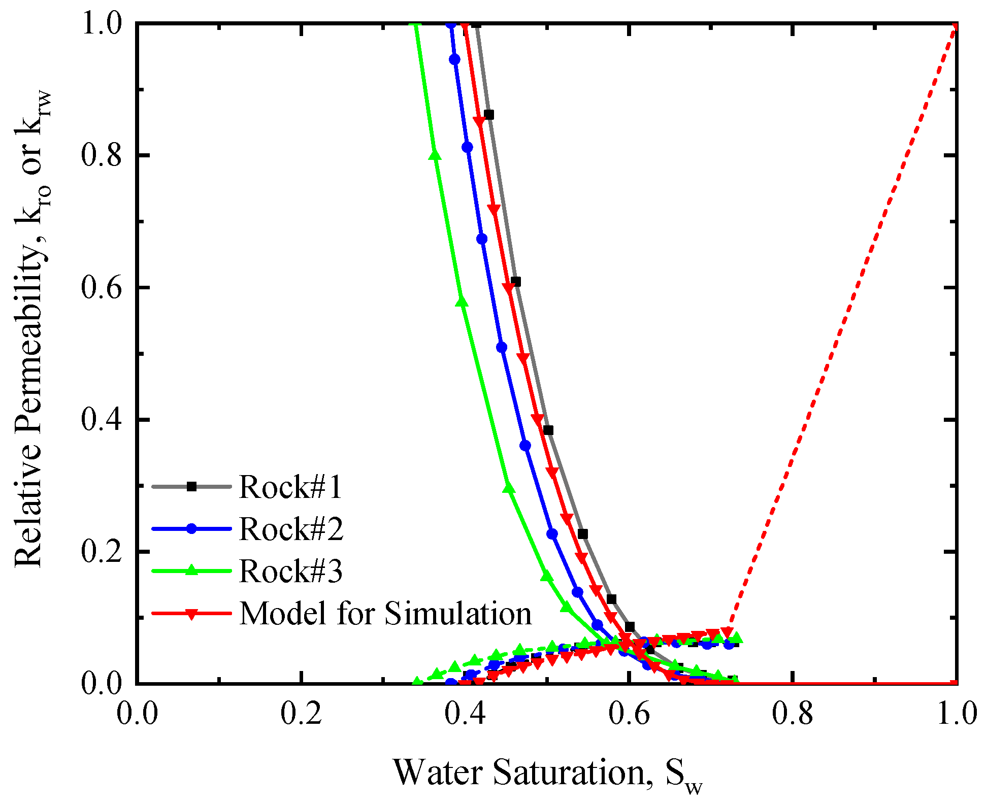
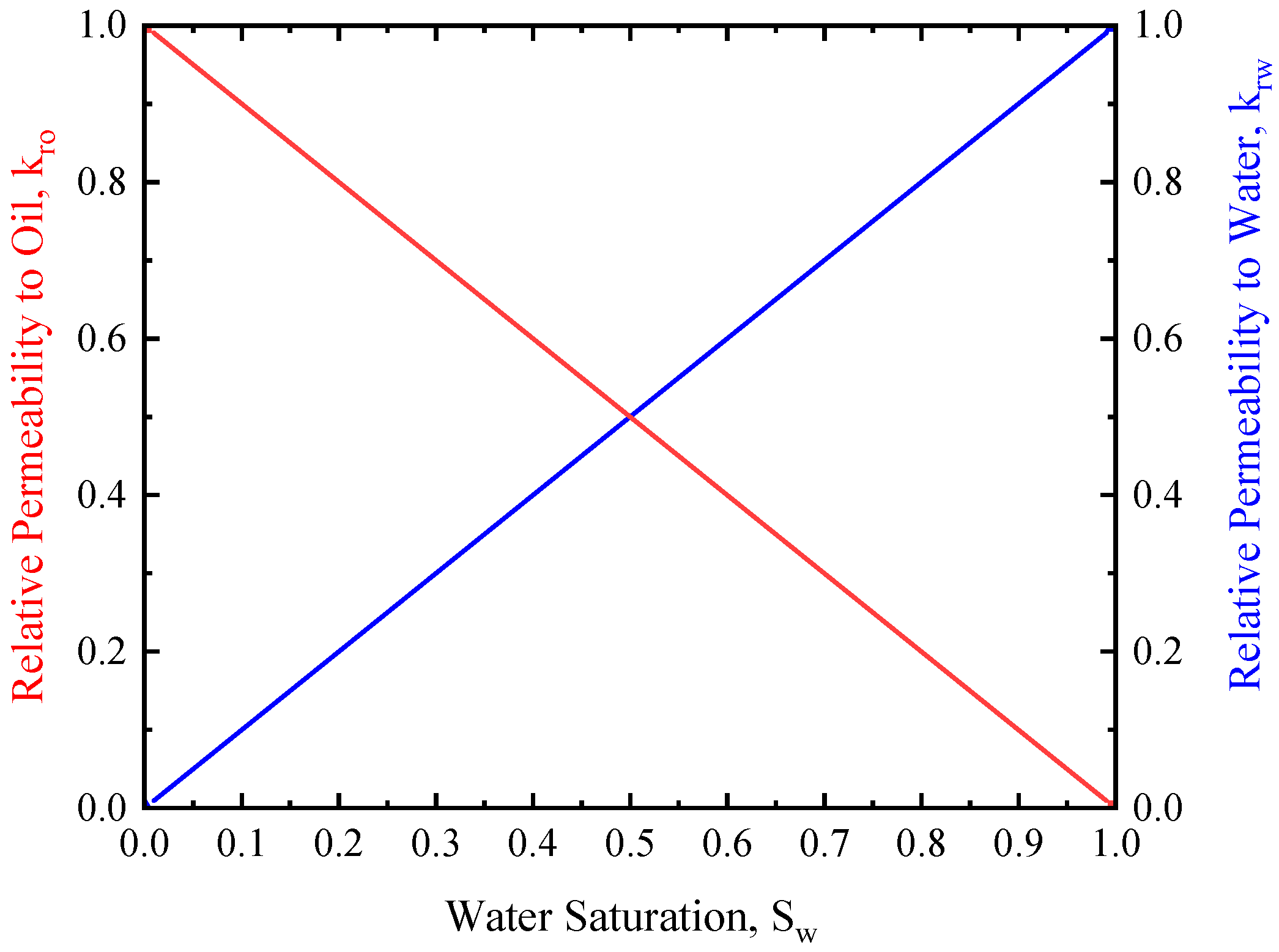
Different relative permeability curves were assigned to the fracture and rock matrix. Relative permeability curves of the rock matrix were measured using the reservoir core samples (Figure 4), while a pair of straight lines was used for hydraulic fractures (Figure 5). The measured relative permeability curves show a limited multiphase flow region for such a low-permeability rock, where the average residual water saturation is around 38%, and the average residual oil saturation is around 27%.

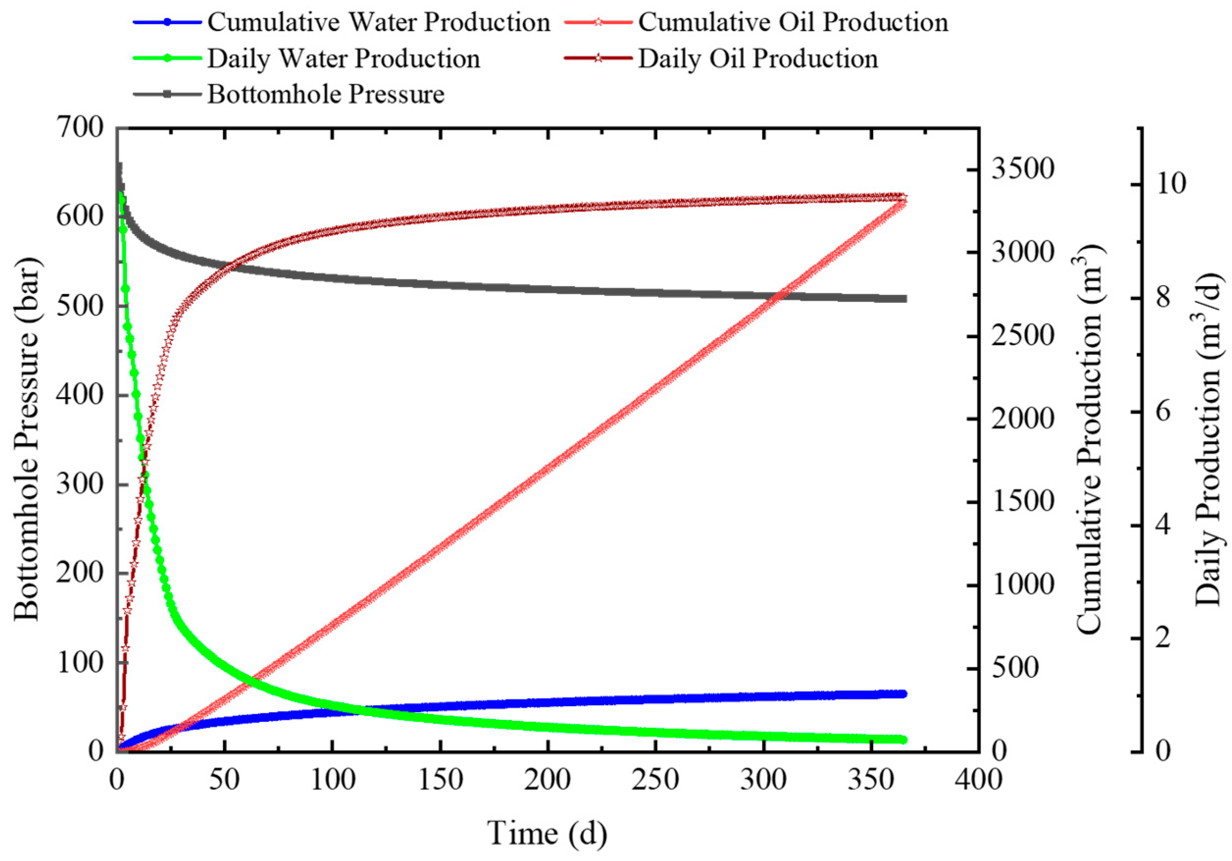
(5) During the production simulation, the production rate was kept at 50 m³/d until the bottom-hole pressure decayed to 35 MPa, after which the production was continued at a constant pressure mode. The calculated production data are shown in Figure 6. As shown in the Figure 6, the daily production of water (i.e., the fracturing fluid) is large in the first 15 days, which represents the main flowback region; in this region, flowback water is mainly from the propped fractures. As production continued, the daily water production decreased and daily oil production increased; after 10 days of production, the oil–water ratio increased beyond 1 in this simulation case.

3.2. Flowback Pattern of the Fracturing Fluid

Along with the production, the fracturing fluid flows back with the oil. Typically, the early flowback has a large water saturation and gradually decreases with time as shown above. Numerical simulation reveals two stages in the production; in the first stage, the flowback water mainly comes from hydraulic fractures, while in the second stage the flowback water mainly comes from the rock matrix. Flowback in the first stage shows the geometry and permeability of the fracture network, while flowback in the second stage shows the geometry and permeability of both the fracture network and the rock matrix.

(1)

Flowback Pattern of the Fracturing Fluid from Hydraulic Fractures

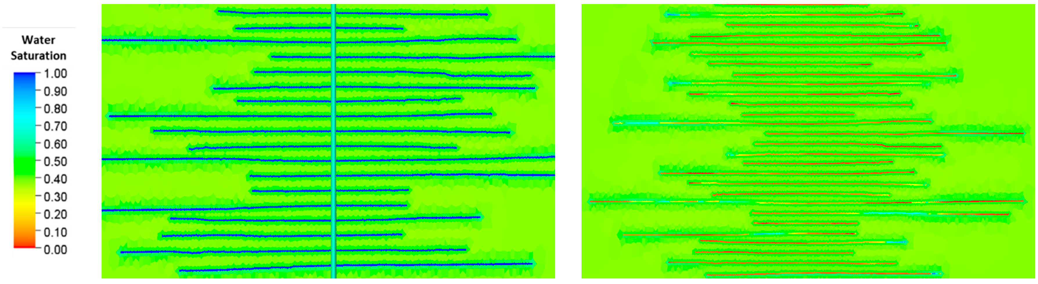
A simple double-wing fracture model is firstly used to understand water flowback after hydraulic fracturing. From the change in water saturation in different grids, it can be seen that after approximately 15 days, water saturation in the fracture drops quickly to around 0 (i.e., residual water saturation as shown in Figure 7), indicating that fracturing fluid in the fracture has almost completely flowed back. However, there is still a large amount of fracturing fluid waiting to flow back in the invaded region adjacent to the fracture.

Using the porosity and water saturation of the fracture grids, the reduction in the fracturing fluid in fractures during the flowback can be determined and compared with the cumulative produced water at the wellhead. During the early stage of flowback, the reduction in hydraulic fracturing fluid within the fracture is slightly less than the cumulative water production at the wellhead; this is because the pore pressure of fractures is larger than the matrix after fracturing, which drives water to imbibe the rock matrix adjacent to fractures. After 17 days of flowback, the cumulative water production at the wellhead exceeded the reduction in hydraulic fracturing fluid within the fracture, indicating that all of the hydraulic fracturing fluid within the fracture had flowed back. At this point, the volume of hydraulic fracturing fluid within the fracture remained relatively stable, and the hydraulic fracturing fluid at the wellhead was supplied by the surrounding invaded zone. As shown in Figure 8, the time point of significant difference between the two curves occurred between 10 and 11 days of flowback, indicating the transition period during which the surrounding invaded zone began to contribute to the flowback of the fracturing fluid.

When we plot the change in the flowback ratio in fractures (i.e., the daily reduction volume of fracturing fluid in fractures to the initial volume of fracturing fluid in fractures), it can be seen that the flowback ratio decreases almost linearly at the early stage but logarithmically at the later stage. These two stages are more obvious in the log–log plot as shown in Figure 9, where the first stage represents the linear flow of the flowback from fractures, and the later stage represents the flowback from the low-permeability rock matrix. The transition between the two stages lasts for several days.

(2)

Flowback Pattern of the Fracturing Fluid from the Invaded Rock Matrix

After 17 days of production, the amount of fracturing fluid in the fracture remains relatively stable. At this point, the flowback rate of the fracturing fluid from the invading region can be calculated, which is approximately equal to the daily water production rate observed at the wellhead. This stage of flowback continues for a long time. After another 100 days of production, the average daily water production at the wellhead is 18.25 m³/d, which can be considered as the return rate of the fracturing fluid from the invaded zone under the current production regime.

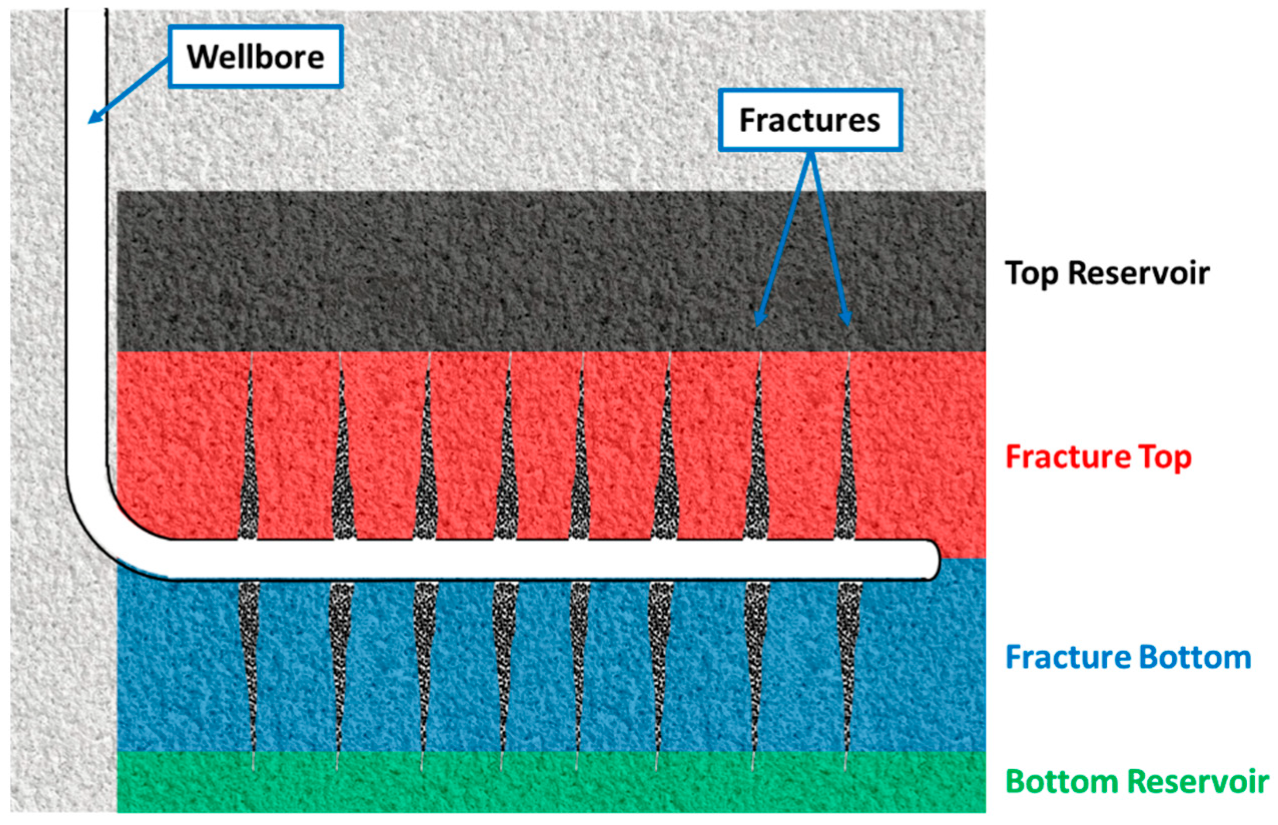
Vertically, the invaded zone where the fracturing fluid invades can be divided into four regions as shown in Figure 10: the reservoir above the fracture, the reservoir surrounding the upper half of the fracture, the reservoir surrounding the lower half of the fracture, and the reservoir below the fracture. Contributions of the fracturing fluid flowing back from these regions change with the production as shown in Figure 11. At the beginning of flowback and production, the fracturing fluid imbibes the reservoir rock due to the high pressure in the fractures, which leads to negative initial flowback rates in the top and bottom reservoir regions; due to gravity, the amount of fracturing fluid imbibing the bottom region of the reservoir is larger than that imbibing the top region of the reservoir. The specific difference is influenced by the reservoir’s permeability, the total amount of fracturing fluid, and pore pressure changes in fractures after hydraulic fractures. In this numerical simulation model, the amount of fracturing fluid that enters the reservoir below the fracture is tens of times larger than the amount that enters the reservoir above the fracture.

When the second flowback stage starts, the fracturing fluid mainly comes from the rock matrix, and imbibition of the fracturing fluid continues, especially in the lower reservoir region due to gravity. In the early period of this stage, the pressure in fractures and their adjacent regions is still high, and the capillary force also plays a role; thus, the fracturing fluid overcomes the gravity and stays in the reservoir above the fracture. However, in the later period of this stage, after the pressure and water saturation around the fracture decrease significantly, the fracturing fluid in the reservoir above the fractures gradually flows back (after 10 months).

3.3. Validation of Flowback Model for Single Cluster

To minimize the interference among fractures, a single-cluster fracturing simulation is conducted to validate the proposed flowback model. Figure 12 shows the changes in production and bottom-hole pressure of this single-cluster case.

The production data are normalized to obtain the rate-normalized pressure (RNP) and material-balance-time (MBT) as shown below:

$$RNP=\frac{p_i-p_{wf}}{q_s} MBT=\frac{N_p}{q_s}$$

After converting the data into MBT and RNP, a plot of the MBT–RNP curve (also known as the flowback characteristic curve) can be generated as shown in Figure 13. The MBT–RNP curve for a cluster shows a good linear trend in the later stages, as expected.

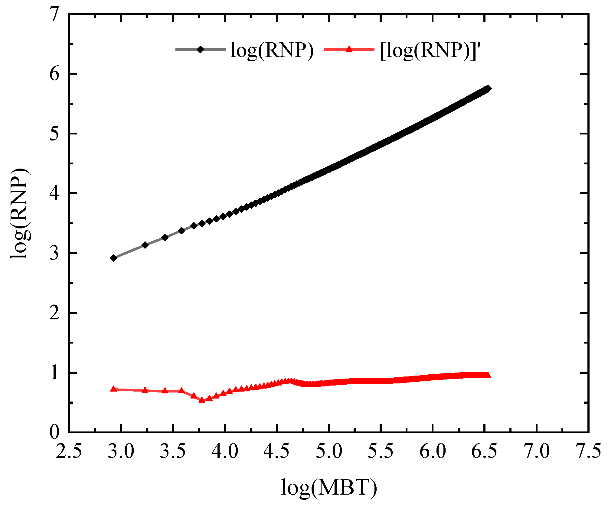
Taking the logarithm of both x and y axes, Figure 13 is converted to a plot of logMBT versus logRNP, as shown in Figure 14. The red curve in Figure 14 shows the change in the slope, which is slightly below 1 before 4.5, and plateaus at 1 thereafter. The slope below 1 is likely attributed to the closure of the fracture at the early stage; once the dimension of the fracture is stabilized, the flowback is a standard linear flow and the slope equals 1.

3.4. Validation of Flowback Model for the Entire Well

Figure 15 shows the flowback characteristic curve of the entire-well case that is calculated from Figure 6. Similar to the single-cluster case, the RNP increases almost linearly with the MBT while the slope changes only slightly at the early stage.

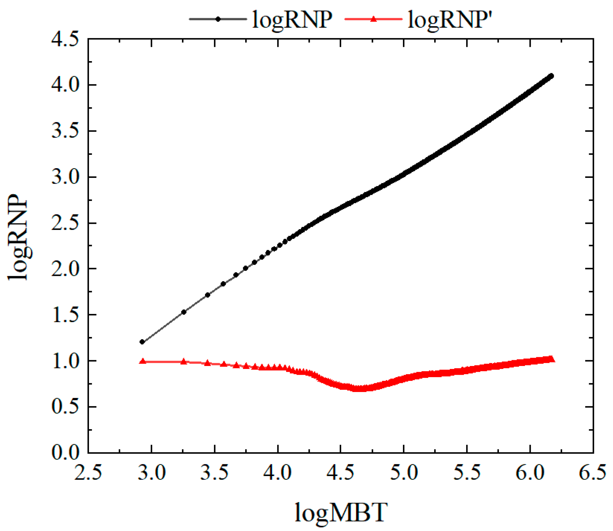
After converting this flowback characteristic curve in the log–log plot as shown in Figure 16, it can be seen that the trend of the logRNP-logMBT of the entire-well case is similar to that of the single-cluster case. By carefully comparing the detailed characteristics of the flowback curve and the fracture network generated by the simulator, it can be found that the flowback data of the single-cluster case are close to those predicted by the ideal mathematical model; however, for the entire-well case, the characteristics of the flowback curve change due to the heterogeneity of the created fractures and their interactions. As shown in Figure 16, the minimal slope of the logRNP-logMBT curve appears after 4.5, which is clearly later than the single-cluster case; this indicates a slower transition to the second stage of the flowback that is mainly determined by the invaded water in the rock matrix.

Furthermore, the total volume of the created fracture network can be calculated based on the slope of the RNP curve in the early stages of the flowback, whose detailed steps are as follows.

(1) Obtain the slope of the RNP curve and the corresponding bottom-hole pressure.

(2) Calculate the compressibility coefficient of the fracture system based on the bottom-hole pressure drop.

(3) Calculate the volume of the fracture network based on the slope and compressibility coefficient.

As shown in Figure 17, when calculating the slope, it is best to select the early flowback data. However, due to the limitation of data acquisition frequency in the field, hourly data are unachievable; instead, fitting data are used which are obtained from the average daily data in the first 10 days of flowback.

In the first few days, the slope (m) of the RNP curve is about 0.0214. An early-proposed empirical formula is used to calculate the compressibility coefficient of the fracture system, which is about 0.00201 MPa⁻¹ [25]. Assuming that the fluid compressibility (C_w) is a constant of 2.59 × 10⁻⁶ MPa⁻¹ and the volume factor B is a constant of 1.02, the total volume of the fracture system can be calculated by (25). which is about 3761.9 m³.

$$V_m=\frac{B}{m\left(C_w+C_f\right)}$$

(25)

In numerical simulation, the total fracture volume is 3066.0 m³, which gives an error of about 22%. Because the empirical formula is established for tight sandstones that are different from the target reservoir, the compressibility coefficient of the fracture system is corrected using the fracture volume from the simulation, which gives 0.00246 MPa⁻¹ for future usage.

4. The Impact of Fracture Complexity

In the horizontal well-fracturing of tight conglomerate reservoirs in the Mahu well area, complex fracture networks are likely to be generated due to the heterogeneous nature of the conglomerate. In fracturing designs, complex fracture networks are not considered, and instead, fractures are assumed to propagate symmetrically with bi-wing fractures. Therefore, we start from such a fracturing design and use natural fractures to generate the complex fracture network formed in tight conglomerate reservoirs. In this section, the density of natural fractures is changed to enable us to understand how it affects the flowback curve.

The natural fracture density comparison is shown in Figure 18, with reservoir properties and fracturing parameters being consistent with those used in previous sections. The key parameters of hydraulic fractures are shown in

Table 4. Hydraulic fracture parameters under different natural fracture densities.

Natural Fracture Densities	Fracture Volume (m3)	Total Fracture Area (m2)	Average Fracture Length (m)	Average Fracture Width (mm)	Average Fracture Conductivity (mD∙m)
None	3066.00	334,861.60	277.83	9.37	660.66
Sparse	2649.00	324,490.60	193.61	8.80	618.30
Dense	2378.00	328,308.80	182.64	8.07	567.21

.

As shown in Figure 19, in the absence of natural fractures, the hydraulic fracturing creates symmetrical bi-wing fractures. The denser the natural fractures are, the more complex the created fracture with shorter fracture lengths, narrower fracture widths, lower fracture conductivities, smaller total fracture volumes, and greater fluid loss will be. However, the total fracture surface area remains approximately equal in all three cases.

Using the same numerical simulation procedure as in Section 2.1, a post-fracturing production simulation is conducted, and the production curves are shown in Figure 20.

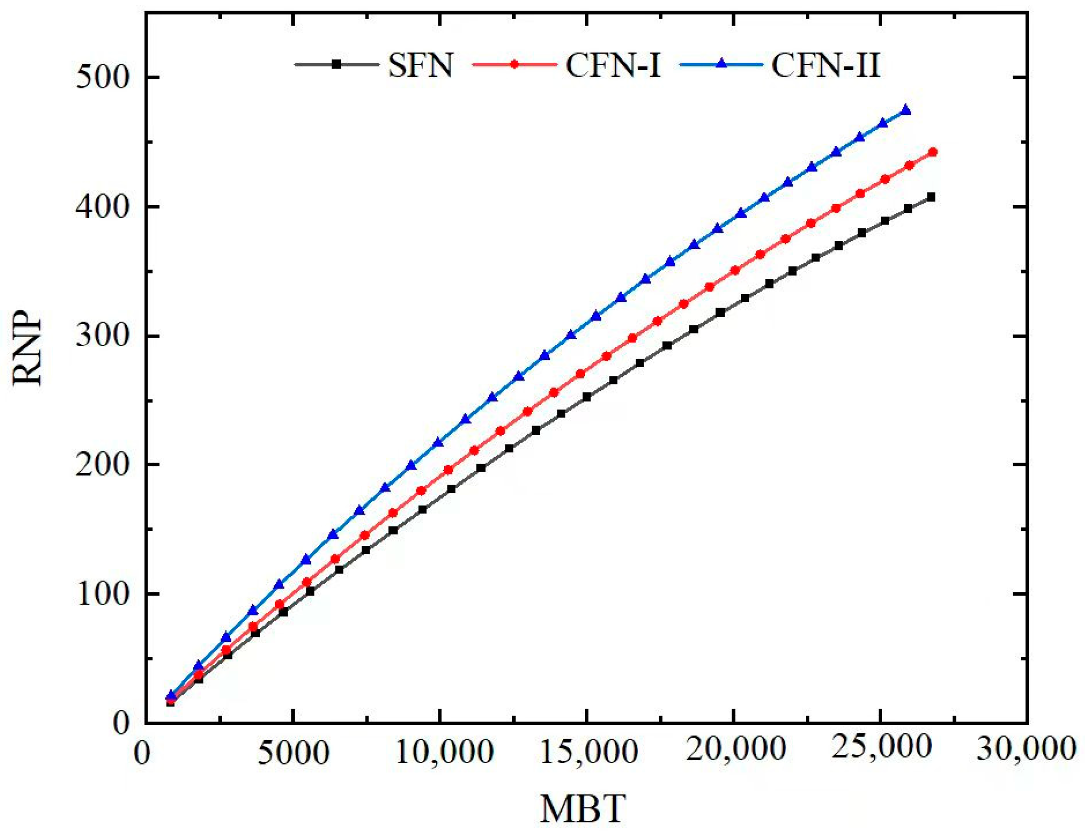
The degree of fracturing complexity is also reflected in the MBT–RNP plot, as well as the log–log plot shown in Figure 21 and Figure 22. The degree of complexity of fractures does not significantly affect the overall trend of the MBT–RNP curve. As shown in Figure 23, as the complexity of the fractures increases, the MBT–RNP curve shifts upwards with a smaller initial slope. Despite this, the initial slope can still be used to accurately calculate the volume of fractures.

The effect of fracture complexity on the MBT–RNP double-logarithmic curve trend is negligible, as the overall trend remains constant. However, the position of the MBT–RNP double-logarithmic curve shifts upward with the increasing fracture complexity. This upward shift is attributed to the increased resistance to fluid flow due to the tortuous path of the fracture. Furthermore, the initial slope of the derivative curve for complex fractures is less than 1, indicating that the linear flow is not present during the initial flowback phase. This non-linear flow behavior is due to the flow resistance caused by the complex fracture path. Water imbibes the matrix adjacent to the fracture network due to the capillary force, which decreases water saturation in hydraulic fractures. The more complex the fracture network is, the bigger the fracture volume is, the longer the time water remains in the formation, the harder the flowback and the lower the flowback ratio will be.

As shown in Figure 24, comparing the logMBT-logRNP’ slope for fractures with different complexities, it is observed that the slope decreases as the fracture complexity increases. This is because the flow path of the fracturing fluid becomes more complex as the fracture complexity increases, resulting in a greater deviation from linear flow in the characteristic curve. Accurate measurement of the MBT–RNP double-logarithmic curve and logMBT-logRNP’ slope for complex fractures is essential for modeling the flowback of the fracturing fluid, which in turn is necessary for calculating the total volume of the fracture network.

5. Conclusions

During hydraulic fracturing, the pressure differential between the fracture and the reservoir can result in a significant loss of fracturing fluid into the formation, particularly adjacent to the fracture faces. During the shut-in, the fluid imbibes the rock matrix from hydraulic fractures, while during the flowback, the fluid quickly returns to fractures and the wellhead. To accurately model the flowback of the fracturing fluid, early and late-time flowback models were developed based on the principles of linear flow within the fracture and from the matrix into the fracture. Notably, the determination of the linear flow is based on the slope of the log–log plot of the MBT versus the RNP curve, which is equal to 1. To achieve greater precision in calculating the total volume of the fracture network, it is essential to obtain accurate pressure and production data in the first few days of the flowback, where the fracturing fluid mainly comes from the hydraulic fractures. The complexity of the flow path of the fracturing fluid during the initial flowback stage determines the deviation of the characteristic flowback curve from the linear flow region, which enables people to know the complexity of the fracture network from the flowback data. Ultimately, with a precise characterization of the fracture compressibility and the early flowback characteristic curve, the total volume of the fracture network can be calculated using the proposed model in this study. In the future, this model can refer to the grid strategy of the discretization complex domain to establish a three-dimensional heterogeneous porous media multiphase flow simulation method.