

Counting Abalone with High Precision Using YOLOv3 and DeepSORT
Department of Industrial Engineering, Chosun University, Gwangju 61452, Republic of Korea
*
Author to whom correspondence should be addressed.
Processes 2023, 11(8), 2351; https://doi.org/10.3390/pr11082351
Submission received: 23 May 2023
/
Revised: 2 August 2023
/
Accepted: 2 August 2023
/
Published: 4 August 2023
(This article belongs to the Topic Advanced Operation, Control, and Planning of Intelligent Energy Systems)
Abstract
:In this research work, an approach using You Only Look Once version three (YOLOv3)-TensorFlow for abalone detection and Deep Simple Online Real-time Tracking (DeepSORT) for abalone tracking in conveyor belt systems is proposed. The conveyor belt system works in coordination with the cameras used to detect abalones. Considering the computational effectiveness and improved detection algorithms, this proposal is promising compared to the previously proposed methods. Some of these methods have low effectiveness and accuracy, and they provide an incorrect counting rate because some of the abalones tend to entangle, resulting in counting two or more abalones as one. Conducting detection and tracking research is crucial to achieve modern solutions for small- and large-scale fishing industries that enable them to accomplish higher automation, non-invasiveness, and low cost. This study is based on the development and improvement of counting analysis tools for automation in the fishing industry. This enhances agility and generates more income without the cost created by inaccuracy.
1. Introduction
The abalone is a single-shelled gastropod mollusk marine snail, which is notable not only for resembling the human ear, but also for being one of the most valuable shellfish in the world. Its high value arises from its good taste and beautiful shell [1]. Generally, abalones live in rocky environments under the sea, where they can feed on algae. The tough and strong shells of abalones create an immensely strong attachment to rocks in the sea, which requires time and skill to remove them during fishing. The abalone is sold in the Korean fish market, and is highly valued as a delicacy and also owing to the difficulty in capturing it in its natural habitat [2]. Therefore, the abalone is one of promising species for sea farming.
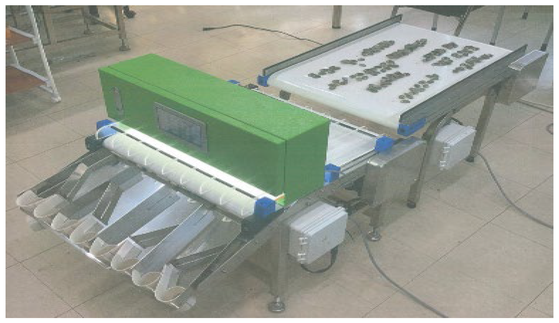
The culturing of abalones comprises two steps: a first nursery and a second nursery. Initially, small abalones are fed into indoor tanks in the first nursery stage, and then the secondary nursery is carried out in the sea as a form of sea farming. The raised abalone, which reaches approximately 1.5 cm or more after the first nursery, is handed over to the second nursery and is grown in the sea. Generally, abalones after the first nursery stage are sold to fishermen for the second nursery. However, the counting of abalones for sale by humans is a difficult task because of their small size, and in some cases they tend to be entangled with each other. Therefore, abalones are sold by weight, which is estimated to be equal to the number of abalones. However, counting by weight does not exactly match the actual number of abalones owing to their weight variation. This inaccuracy in counting abalones causes a loss of selling profit, considering their high price. To solve this problem, machines that count abalones automatically have been developed and used (see Figure 1). To operate the counting machine in Figure 1, an algorithm using image sensor and LabVIEW [3] was implemented. In this machine, the installed cameras capture images of moving abalones on a conveyor belt. The captured images are converted to black and white images so that the black area represents the abalones, and the white color represents the empty area. Then, the black area is divided into the average pixel size of an abalone to estimate the number of abalones within the image.
During the growth of abalone in tanks, many abalones tend be entangled, which poses a challenge to counting them on the conveyor belt system with the accuracy required by fishing industries. Therefore, these industries are conducting further research to address the problem of abalone occlusion which results in two or more abalones being counted seen in (Figure 2). In this context, this study proposes an application of the deep learning algorithm for detecting, tracking, and counting moving abalones on a conveyor belt, which is composed of You Only Look Once version three (YOLOv3) as the detector and Deep Simple Online Real-time Tracking (DeepSORT) as the tracker [4].
2. State of the Art
2.1. Object Detection
Object detection has been an essential research topic in many industrial areas such as defect detection, autonomous driving, robot arms, and so on. As the pillar of image understanding through computer vision, object detection is regarded as the basic concept in high-level and is composed of complex tasks such as image captioning, object tracking, segmentation, pattern detection, and motion recognition. Notable conventional methods in research of object detection have been developed from the early studies with several models built as an ensemble of feature extractors, such as the Viola–Jones detector [5] and the histogram of oriented gradients (HOG) [6]. These models are slow, inaccurate, and perform poorly on unknown datasets. Garay et al. [7] proposed an overview of AMR system based in the computational and wireless sensor network. Using a video micro-camera and an Optical Character Recognition (OCR) module included into the sensor node, the AMR system reads the meter’s numerals. The data are transmitted to the management center through ZigBee wireless networks, where communication takes place in a mesh topology. The application of deep learning and convolutional neural networks (CNNs) for image classification has altered the visual recognition outlook. The CNNs used in the ImageNet Large Scale Visual Recognition Challenge (ILSVRC) 2012 challenge by AlexNet provided the groundwork for neural network utilization in computer vision [8]. Currently, the implementation of object recognition ranges from autonomous cars to identification in security systems, medical applications, and more. In recent years, there has been exponential growth in this field with the rapid development of new tools and technologies. Côté-Allard et al. [9] proposed the use of transfer learning for surface electromyography sEMG hand gestures detection using CNN. CNN is augmented using transfer learning method to reduce data generation burden on gesture data. The CNN model resulted in an accuracy of 97.81% on seven hand gestures by 17 participants.
Object detection based on CNNs can be divided into two types depending on whether it uses a region proposal network (RPN): one-stage and two-stage methods [10]. Many two-stage object detection methods are based on determining the region of interest (ROI) [11]. Ren et al. [12] proposed the Faster R-CNN, which achieved substantial improvement and provided the foundation for subsequent studies. Object detection can be framed as a regression problem for spatially separated bounding boxes which represents a specific area in the image for object existence and the associated class probabilities of the bounding box. A single neural network predicts bounding boxes and class probabilities directly from full images in one evaluation. A single-shot detector (SSD) makes it possible to discretize the output space of the bounding boxes into a set of default boxes with different aspect ratios and scales per feature map location [13].
YOLO was introduced by Joseph Redmon et al. [14] who proposed a one-time CNN to predict the frame position, and classify and determine the detected objects among multiple categories (such as humans, cars, bicycles, dogs, or cats). YOLO uses regression to solve object detection, which takes an input image, and learns the class probabilities and bounding box coordinates. Using YOLO, single images are divided into S × S pixel size grids, and each grid predicts the bounding boxes and confidence level. Confidence represents the precision of the bounding box as well as whether the bounding box truly includes an object, regardless of class. YOLO predicts the classification score for each box in each training class. A single end-to-end system completes the process of assigning the output obtained from the original image to a category or position [15].
Zhong et al. [16] stated that deep networks, such as YOLOR-P6 and YOLO-W6, could perform at the highest level as usable on large datasets; however, they attained lower accuracy on limited datasets owing to overfitting. Additionally, they demonstrated that simpler networks such as YOLOv3 and YOLOv5 can achieve better precision. Balakrishnan et al. [17] undertook a comparative study of various YOLO model architectures used in object recognition. The authors compared the Darknet architecture with YOLOv5, YOLOv3, Tiny YOLO, and ResNet under ImageAI library. From their results, the research concluded that YOLO with the Darknet model having weight for trained objects gives better performance. Xu et al. [18] trained a YOLO architecture with three different datasets to identify various fish species and achieved a mean average precision score of 0.5392. Pedersen et al. [19] utilized the YOLO method and expanded their work to include marine mammals and fish. These methodologies train their networks as end-to-end. Shankar et al. [20] compared YOLOv3, YOLOv5, and YOLOv7 architectures for the detection of underwater marine creatures. In this study, these YOLO are chosen due to their excellent detection accuracy and quickness in real-time application for the detection of aquatic species. The study concluded that enhanced YOLOv7 achieved the better performance than other frameworks with the mean average precision (mAP) of 0.82, in the detection of underwater marine creatures.
SSD [13], deconvolution single-shot detector (DSSD) [21], RetinaNet [22], M2Det [23], and RefineDet++ [24] are more recent algorithms based on single-stage object detection. Two-stage detectors typically perform better because they are more powerful and complex than single-stage detectors. In terms of accuracy and inference time, YOLO challenges not only two-stage detectors, but also the earlier single-stage detectors. This is because of its straightforward architectural design, low complexity, and simple implementation, and it is regarded as one of the most prevalent choices in production [25].
2.2. Marine Object Counting with Machines
Object counting machines in small factories or large industrial sites predominantly use conveyor belts for sorting and movement. To automate object counting on the conveyor belt, some of them are equipped with cameras on top of the conveyor belt that acquire video data or images. The acquired videos or images are processed to count the objects in real time.
Some researchers have described how computer vision can be used in the abalone counting process. For instance, Park et al. [3] proposed abalone detection and counting based on LabVIEW machine vision in a conveyor system. They deployed a camera rather than a proximity sensor to count abalones because the existing proximity sensor has an error rate of approximately 3%, depending on the conveying process. This approach presented a promising result for the counting process; however, in some scenarios where abalones are entangled, it leads to inaccurate counting. To address this problem, abalones can be counted manually by separating the entangled ones, but this is impossible in large or automated fisheries because it is time consuming and labor-intensive. Therefore, it is important to address the problem of abalone entanglement.
Tseng et al. [26] classified fish using onboard CCTV videos with a masked region-based CNN (Mask R-CNN) algorithm. Using videos captured on the deck of a long liner, Tseng and Kuo identified a variety of fish with an accuracy of 83% (F1-score) and a counting inaccuracy of 21%. French et al. [27] successfully detected a variety of fish on a conveyor belt within a fishing boat. In a research vessel experiment with known numbers of fish, a mean class accuracy of 63% was obtained, whereas in a commercial vessel, a mean class accuracy of 57–59% was achieved. Humans who participated were reported to have a mean class accuracy between 74% and 86% for a sample dataset.
To create optical systems for fish counting that achieve the required detection and counting rates and address the low signal-to-noise caused by water fluctuations, Klapp et al. [28] combined hybrid non-imaging optics with image processing techniques. They created an embedded system based on the Raspberry Pi and a fixed focus lens to count two types of ornamental fish in an aquarium, ranging in size from 0.5 to 2.3 g, and achieved an accuracy of 94% to 98%.
2.3. Object Counting with Deep Learning
Deep learning algorithms such as CNNs [29] have shown significant advances over traditionally used methods for computer vision tasks, including object detection, pattern recognition, and image classification. In the abalone counting process, a CNN can solve the problem of abalone entanglement through object detection. Abdelwahab [30] proposed an approach related to this research by employing regions with CNN features (R-CNN) for detection and the Kanade–Lucas–Tomasi algorithm (KLT) for counting and tracking vehicles. The R-CNN model with KLT showed promising results for tracking vehicles. The application of these methods in real-world platforms is even more challenging since they require expensive hardware such as robots, high-performance cameras, or computers.
Recently, numerous studies have been conducted on video-based counting frameworks, primarily for automobiles, traffic, and pedestrians. These studies are important because they analyze the state of road traffic and estimate its density. Using four datasets, Hardjono et al. [31] conducted research on vehicle counting using various techniques. With the help of Viola–Jones methods, background subtraction, and already-existing CCTV data, F1 scores ranging from 0.32 to 0.75 were successfully derived from a single low-resolution dataset. The study found that, compared to the background subtraction approach, the Viola–Jones method can increase the F1 score by approximately 39–56%. Using three datasets with higher resolution, the YOLO algorithm also produced better results, with improved F1 scores ranging from 0.94 to 1 and precision ranging from 97.37% to 100%.
To extract edge boxes, Li et al. [32] employed the AlexNet technique with multiple layers and edge boxes. With a false rate of 10% and a missing range of 23%, the box algorithm produced satisfactory results. According to Redmon [14], YOLO is effective on identifying objects in images. Current techniques employ classifiers to detect objects. The PASCAL VOC 2007 and VOC 2012 test sets attained the mAP of 57.9%.
Asha et al. [33] developed a system for counting vehicles in highway traffic using cameras. YOLO object recognition, correlation filter tracking, and counting are three steps used to complete video processing. While their suggested method can properly detect, track, and count vehicles, it does not provide enough processing time estimation, and according to research, it is too slow for real-time processing on edge devices such as the Jetson Nano or Raspberry Pi.
According to Forero et al. [34], research on classification algorithm that tracks and counts cars and pedestrians using video sequences. The authors used the YOLO framework for detection. Using training data with over 5000 labels, the recognition and counting of bicycles in a circumstance of non-occlusion achieved a detection threshold of 97.6% and was only affected when objects were too close together, and it was impossible to distinguish between the groups.
In this sense, our work aims to apply the YOLOv3 and DeepSORT models for counting abalones. Our main contributions are as follows: (1) abalones are counted from the viewpoint of applicability, (2) the current problem of counting entangled abalones is resolved, and (3) a practical solution is provided for counting in the food industry using a conveyor belt. See Table 1 below shows the general comparison of previous works related to marine counting with machine and object counting with deep learning.
3. Model Description
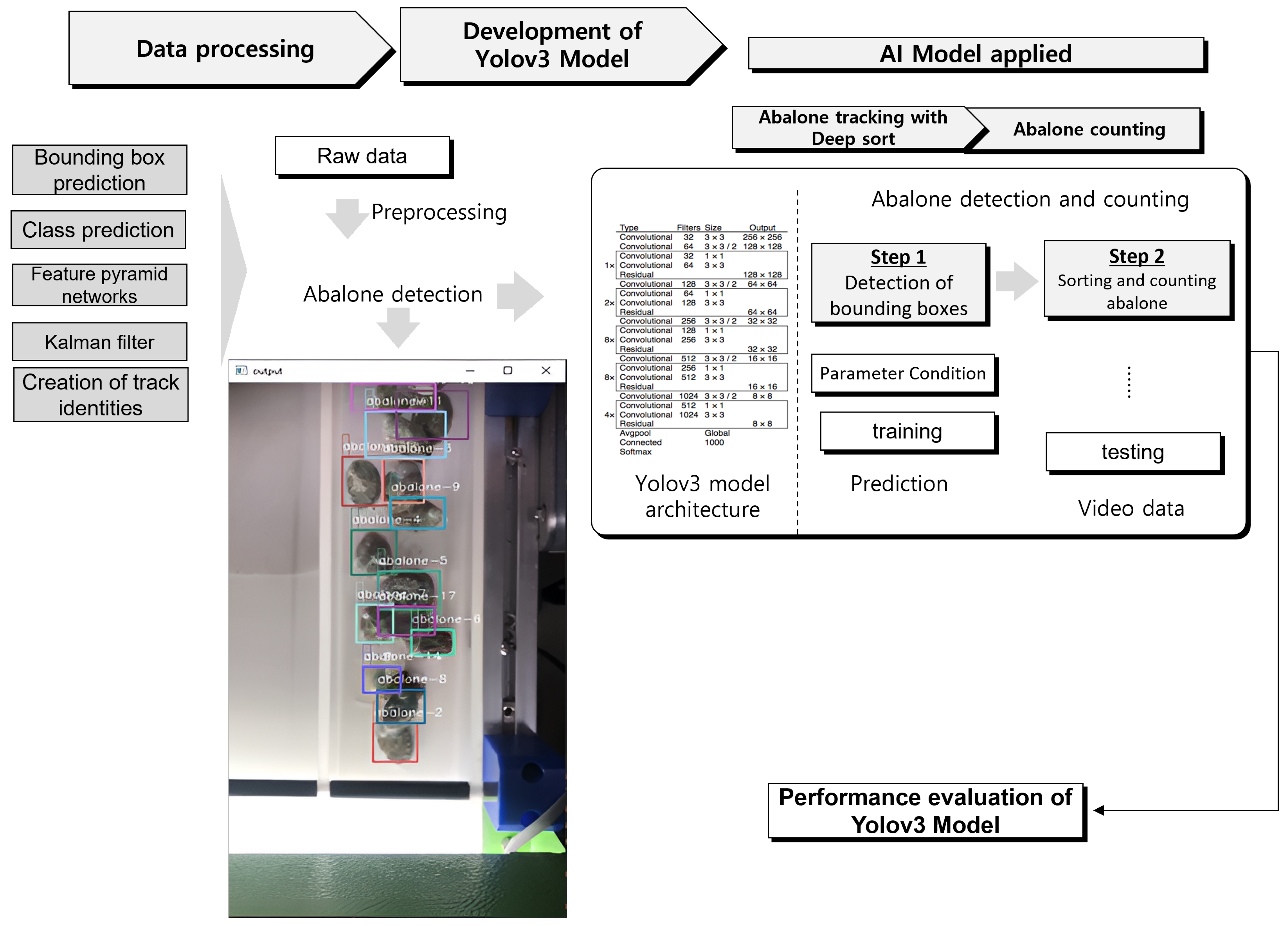
To develop an abalone counting methodology from a video sequence, the components presented in Figure 3 work together. Each component uses a different model, as described in this section.
The first step is data preparation. In this step, datasets with annotated images containing abalone instances are gathered from video data. For building training model, YOLOv3 is set to use TensorFlow. Training is carried out using annotated abalone data. The training process involves feeding the annotated images and their corresponding bounding box annotations into the model, and optimizing the model parameters to accurately detect abalone objects. After training, the performance of YOLOv3 model is evaluated by the separate test set. This step helps in assessing the accuracy and generalization capabilities of developed trained model. In the next step, DeepSORT is integrated. DeepSORT is a tracking algorithm used in conjunction with YOLOv3 to track abalone objects across multiple frames. DeepSORT is integrated with YOLOv3 model to associate bounding box detections across frames and track abalone instances over time. The tracking is performed by applying the combined YOLOv3-DeepSORT model on a video or sequence of image frames containing abalone. The model will detect and track abalone instances, assigning unique IDs to each abalone instance to count, and monitor their movements. The number of unique abalone instances is counted based on their tracked IDs. Each ID represents a distinct abalone object. Summing up the unique IDs will give the count of abalone in the video or sequence of frames.
3.1. Data Architecture for Model Development
Object tracking is the process of tracking single or grouped moving or motionless objects. In recent years, detection has improved owing to the development of artificial neural networks (ANNs) that use complex structures to distinguish patterns in image. The image classification algorithm depicts bounding boxes that represent the locations of objects. The R-CNN presented by Girshick [35] can show different number of regions, as much as 2000, in one image. This study implemented a decoding method to extract all frames as images contained in the targeted video data using the FFmpeg tool [36]. The video sequences used in this study had durations of 16, 18, 20, and 30 s, with 110 to 400 frames. However, owing to the blurriness of the abalone in some frames, approximately 25% of the finally gathered valid frames was discarded. In addition, considering that the number of frames for training in the deep learning model (Darknet-53) is limited to avoid incurring overfitting, a data augmentation technique is applied to increase the number of frames. The data are augmented by rotating each frame from 0° to 90° and changing the saturation, brightness, image flipping, and shearing. The prepared data are divided into 70% for training and 30% for testing.
To generate labeling for image annotation, the LabelImg tool [37] is used, which is written in Python and uses QT for its graphical interface. Each frame is annotated manually. The annotations containing details about the objects in the image, such as image name and label name, image path, class name of the object(s), and coordinates of the bounding boxes surrounding the objects present in the image, are saved as extensible markup language (XML) files in the PASCAL VOC format, which is used by ImageNet. Furthermore, it supports YOLO and creates machine learning (ML) formats [38]. The annotated images are saved with the text files in YOLO format (jpg image files), which contained values such as (object class), (x_center), (y_center), (width), and (height). The class object shows the position of the abalone using integers.
The YOLO format calculates the annotation values using <center-x = x/W>, <center-y = y/H>, <width = w/W>, and <height = h/H>, where the x- and y-coordinates are the centers of the bounding boxes. H and W denote the height and width of the entire image, respectively.
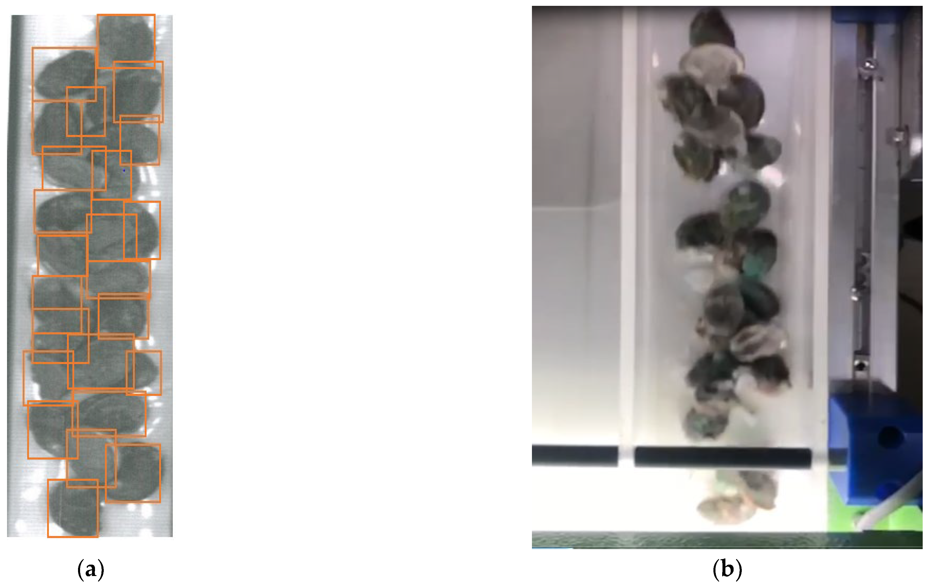
In the second row of Table 2, ‘15’ represents the number of object class for abalone, 0.504950 as the height, 0.729167 as the width, 0.128713 as the x-coordinate (center value), and (0.030556) as the y-coordinate (center value). The orange box on the left side of Figure 4 (a) shows the bounding box for each abalone and (b) show and example of frame in the video data. In the image, each abalone has its own bounding box, and the size and center information are recorded in YOLO format.
3.2. Detection Method
In general, the core of many object detection results is retrieved using Faster R-CNN, which has been acknowledged as one of the best versions [39]. However, real-time image detection and re-association techniques fall short of the real-time tracking requirements owing to the detection speed limitations of Faster R-CNN. YOLO [14] uses the same network both for detection and classification, and this is treated as a single regression problem in contrast to the Faster R-CNN working concept. A direct calculation from the image pixel information to the bounding box coordinates and categories is possible. The supplied image is divided into S × S grids. The grid is in charge of target detection if the target center is located inside the grid. By forecasting the category probability, border, and confidence, it can determine the likelihood of each category being within the border as well as the degree of fit.
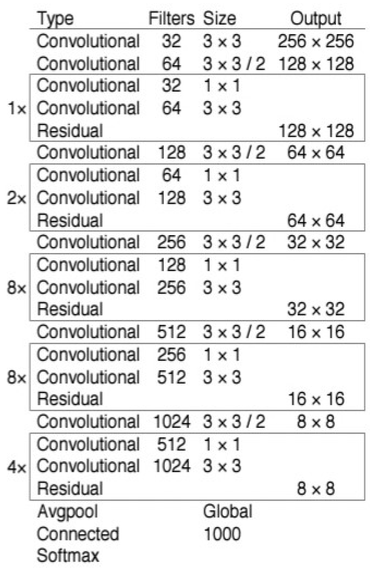
However, many restrictions remain in YOLOv1 [14]. Therefore, the application of YOLOv1 is somewhat constrained. The distance between objects in an image determines the limitations of YOLOv1. It is difficult to identify smaller objects in an image due to clustering. This architecture has issues with object localization and recognition when the dimensions of the object are different from those used for the training data [40,41]. Owing to localization errors, the main aim of YOLOv1 is to identify objects in a given image, whereas in Faster R-CNN, YOLOv2 [42] introduced the concept of an anchor box to increase the positioning performance. YOLOv2 employs a clustering approach that determines the size of the anchor box for the associated dataset, which enhances positioning accuracy. Batch normalization is implemented across all convolutional layers in YOLOv2, which improves the model convergence and boosts the input resolution, allowing the network to recognize higher-quality images more effectively. The YOLO [14], YOLOv2 [42], and YOLOv3 [25] networks introduce three separate scale detections based on the principles of the feature pyramid network (FPN), which correlates with targets of various sizes. To enable each detection block to predict several categories, multiple distinct logical classifiers are utilized instead of the Soft-max classifier. The network’s detection accuracy has significantly increased since YOLOv3 incorporates a Darknet-53 [25] backbone, which is a network architecture with 53 convolution layers (see Figure 5). Therefore, the YOLOv3 network is employed as the detection module in this study to ensure detection speed and accuracy. It adapts better to new scenes and has a greater effect on high-resolution input images.
3.3. Multiple Object Tracking
As stated by Dadhich [43], multiple object tracking (MOT) can be used for detection and association. DeepSORT is a widely used model that introduces another association of apparent feature information in which the appearance of new detections is compared with that of previously tracked objects in each track to aid in the data association problem where there are occluded objects or crowded environments within a frame. Since the performance of the deep network used to extract apparent features has a direct impact on the distribution of slow or rapid movements of objects (tracking technique), this study offers a wide-residual-inception network with improved performance, fewer parameters, and quicker computation. This network extends the previous network by adding an inception structure, making it deeper and wider. It can extract features of varied sizes and make the network more discriminative using convolution kernels of varying sizes. Only the feature extraction element of the network is preserved after removing the original detection module, and the network eventually produces a 128-dimension feature vector [44] that is compatible with a wide-residual network.
Fusion matching of the motion and apparent features is used to associate the target detection results with the tracker. The degree of motion matching matches the tracker location information with the detection results. When the motion matching feature is smaller than the training threshold, the detection frame is regarded as successfully matching the prediction frame of the preceding frame detection result. When only the motion matching feature is employed, the prediction frame cannot be effectively matched with the detection frame when the target has an occlusion, and when the target’s occlusion is removed, the tracker immediately allocates a new ID to the target. Consequently, the characteristic of apparent matching is employed to match the tracker’s identity information with the detection results. The detection frame is regarded as belonging to the existing track when the feature of the apparent matching between the detection frame and trajectory in the current trajectory space is less than the training threshold. In this method, after successfully associating the motion state feature with the target of normal motion, the apparent feature is utilized to determine whether the target belongs to a trajectory. The previous trajectory ID (the direction of the object in the frame) for the occluded target can be re-associated using the apparent feature after the target occlusion vanishes.
It is crucial to give each new target a unique ID while performing multitarget tracking as well as to prevent the target’s track update from quickly disappearing from the screen. A new tracker pertaining to the target is created in the experiment when the trajectory prediction frame of the target in the next three frames of the images can be associated with the detection frame. If there is no association success at the following time, it is termed a false alarm and the detection box is removed. For each current track, if an image cannot be accurately associated with a tracking track for 60 consecutive frames for each existing tracking track, it is decided that the target has vanished, and the track space corresponding to that feature space is wiped.
3.4. Counting Model Architecture
Although Park et al. [3] and Abdelwahab [30] showed promising results, our proposed approach can show improvements in these results by using YOLOv3 (Figure 6) for abalone detection and a robust DeepSORT model for tracking the detected abalones. The method proposed by Park et al. [3] has already been shown to be useful in the problem of counting abalones using the LabVIEW approach, and the study conducted by Abdelwahab obtained promising results from counting people. These approaches are similar to that used in this study.
In this study, the model is validated for detecting entangled and counted abalones. In the tested case, the base results show that the YOLOv3 confidence score influences the level of detection of single and entangled abalones, thereby influencing the counting accuracy. The YOLOv3 backbone, Darknet-53, combines a deep neural network and a convolutional layer. The FPN fuses the features that the convolution layer extracts from an image. The neck is performed by the FPN. Given that it includes numerous bottom-up and top-down pathways, the neck is important for extracting feature maps from various stages, whereas the head contains YOLO maps. Based on the width, height, class label, and probability of each class in the bounding box coordinates, the head determines the final prediction as part of a one-stage detector.
4. Experiments and Results
4.1. Detection Model Training
The experiment on the proposed model is performed using Google Collaboratory, which is an open-source free access to computational resources, such as a GPU, which requires no configuration. Ro-boflow.ai, a free tool that enables developers to create limitless computer vision applications built on YOLOv3, is used. During the training of the model, the number of epochs to be learned and the stack size used to train the top layers of the model in detecting abalone classes are changed. Training the model for 300 epochs requires approximately 120 min.
The mean average precision (mAP), F1 score, and recall with precision curve are used to assess the model accuracy. It is crucial to examine the results of the model classification (confusion matrix) and localization using the IoU of the bounding boxes in the image metrics. The intersection of union (IoU) is essential for object detection. The IoU calculates the intersection over the union of the two bounding boxes, that is, the predicted bounding box and the ground truth bounding box. When the IoU is 1, the ground truth and predicted bounding boxes completely overlap.
A bounding box is drawn around the object only when the IoU exceeds a predefined threshold value. In this application, the IoU threshold is set to 0.4. As a result, detection is classified as true positive (TP) when the IoU is greater than 0.4, and false positive (FP) when the IoU is less than 0.4. False negatives (FN) occur when a model fails to recognize an object in an image while accessing the ground truth. Any area where no object can be expected is considered a true negative (TN) of the image. However, this method does not aid object detection. Therefore, TN is disregarded in Equation (1).
The precision is defined as the ratio of correctly classified positive samples to all positive samples, whether correctly or incorrectly classified. Equation (2) quantifies the precision with which a model classifies a sample as positive.
The recall is calculated by dividing the number of positive samples correctly classified as positive by the total number of positive samples. This is expressed by Equation (3), which represents how well the model detects positive samples.
The accuracy and recall of each observation are used to determine F1 scores. A score of one indicates the highest accuracy, as shown in Equation (4).
The precision–recall curve is given when the recall increases and the precision decreases, meaning that when the positive values increase as the maximum recall increases, the accuracy of identifying the values decreases, indicating minimum precision.
The mean average precision (mAP) score is computed by comparing the detected bounding box with the ground truth of the bounding box. The higher the score, the better is the model detection. This is shown in Equation (4),
where n is the number of classes and APK is the average precision of class k. The mAP scores for the YOLOv3 model were 0.978 (@0.5 mAP) and 0.583 (@0.95 mAP), and the F1-confidence score is 0.95.
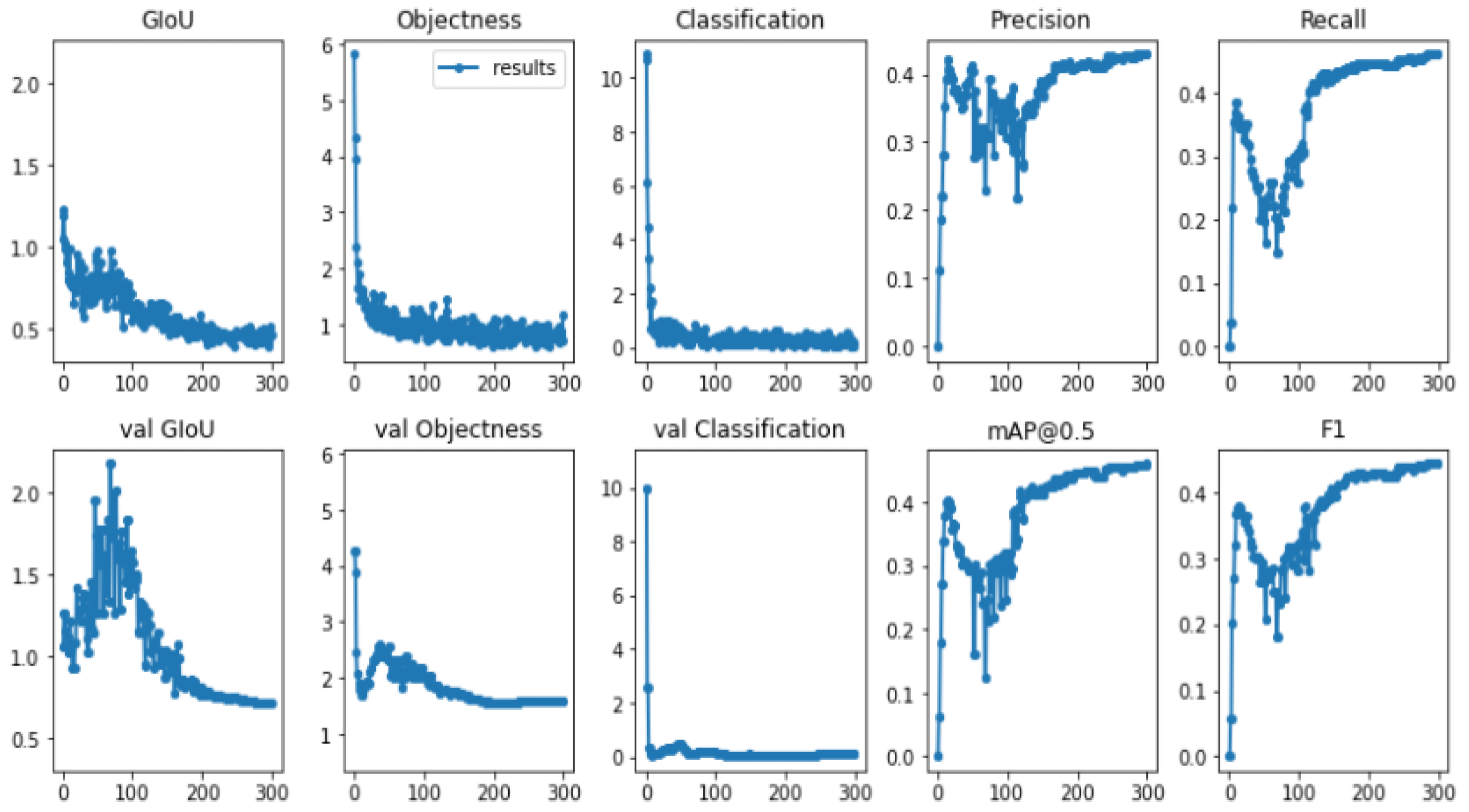
By adjusting the training parameters, some improvements in the model are observed (see Figure 7). The multiple performance metrics for the training datasets are shown in Figure 7.
The performance evaluation graphs for precision, classification, objectness loss, F1 score, recall, and mean average precision (mAP) of the training and validation sets are shown in Figure 7. Figure 7 shows three basic types of loss: categorization, objectness, and GIoU loss (Generalized Intersection of Union). The ideal bounding box regression loss is represented by the GIoU loss. The reduced bounding regression loss indicates that accuracy improves consistently [45]. Objectness loss is a measure of the likelihood that an object exists in a suggested region of interest. If objectivity is high, an object is probably present in the image. Classification loss indicates the effectiveness of an algorithm in predicting the proper class of a given object. Therefore, the lower the GIoU, objectness, and classification, the higher the mAP and F1 scores from the model.
The model improved swiftly in terms of precision, recall, mean average precision, and F1 score before reaching approximately 150 epochs. The box, objectness, and classification losses of the training data rapidly declined until approximately 300 epochs. Therefore, early stopping was applied during training to select the best weights.
After training the proposed model, predictions are performed for the test datasets. The images are resized to 416 pixels × 416 pixels. The batch size is set to 16. The learning rate is set as 0.0001, and stochastic gradient descent (SGD) is the adopted optimizer. The dataset is trained using the pre-trained weights YOLOv3.pt. The examples in Figure 8 show that the proposed model could detect most abalones in the frames with a higher degree of certainty. This shows improved results in recognizing the single and occluded abalones.
4.2. Tracking
Tracking is a method of predicting the locations of objects in a video using both spatial and temporal data. Tracking, in more technical terms, involves receiving the initial set of detections, assigning unique IDs to them, and tracking them over the frames of the video stream while keeping the allocated IDs. In this study, tracking is essential due to the occlusion of the abalone in some frames of the video data. When using an object detector such as YOLOv3, it simply displays where the objects in the frames are; while looking at the array of outputs, the coordinates corresponding to the objects in the bounding boxes will not be seen. A tracker assigns an ID to each object, and it tracks and maintains the ID for the duration of that object’s lifespan in that frame.
DeepSORT is a computer vision tracking technique that tracks objects while assigning an ID to each one in a frame. DeepSORT incorporates deep learning into a SORT algorithm by including an appearance descriptor to decrease the number of identity swaps of objects in frames, making tracking more efficient. In the object-estimation step, the detections from one frame to the next use a constant-velocity model to estimate the target’s position in the following frame. When a detection is associated with a target, the detected bounding box is used to update the target state, and the velocity components are addressed using the Kalman filter algorithm [46].
To characterize the motion state, DeepSORT employs the parameters (u, v, γ, h, x’, y’, γ‘, h’), where (u, v) are the bounding box’s center coordinates, (γ) is the aspect ratio, and (h) is the height. In the picture coordinate system, the remaining four variables denote the velocity data. To anticipate the desired motion state, this method employs a conventional Kalman filter based on a constant-velocity model and a linear observation model (u, v, γ, h).
An appearance descriptor is used to extract features from the detected images and track objects. A CNN trained on large-scale re-identification datasets serves as the appearance descriptor. It extracts features such that features from the same identity are close together in the feature space, whereas features from other identities are far apart.
Researchers of DeepSORT have suggested the association of spatial and appearance information to obtain new detections with a higher confidence. Equation (5) represents the spatial information.
d(1)(i, j) = (dj − yi)TSi−1(dj − yi)
The projection of the ith track in the space of measurements is denoted by (yi, Si), and the jth new detection is denoted by (dj). The distance measured in the Mahalanobis function calculates the uncertainty length between the jth new detection and the ith track’s projected location by the standard deviation. Equation (6) represents the appearance information.
where r is the appearance descriptor, and (Ri) is the appearance of the last 100 objects in a frame connected to the ith track. Each distance is accompanied by gate matrices and , which are equal to 1 if the distance is less than a predetermined threshold, and 0 otherwise.
Finally, to obtain new detections from existing tracks, DeepSORT uses the cost and gate matrix represented in Equation (7).
ci,j = λd(1)(i, j) + (1 − λ)d(2)(i, j)
The gate matrices and , which are equal to 1 if the distance is less than a predetermined threshold, and 0 otherwise, show that new detections are linked to existing tracks.
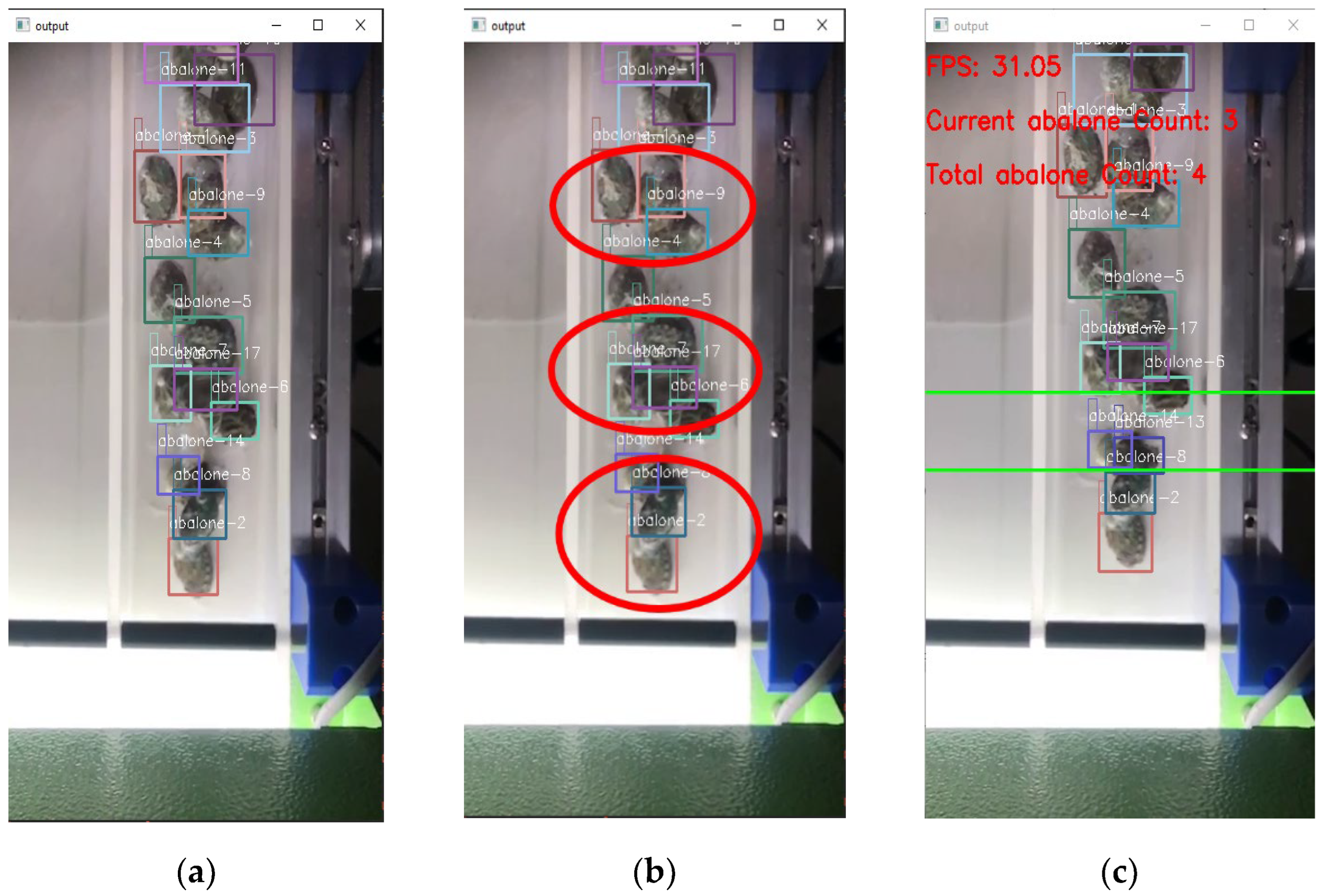
For the abalone count, two lines are drawn in the middle of the frame to show that if the abalone passes between the two lines (region), each abalone will be counted as one. The total count of abalones and frames per second (fps) are displayed on the video frame [30].
5. Results and Analysis
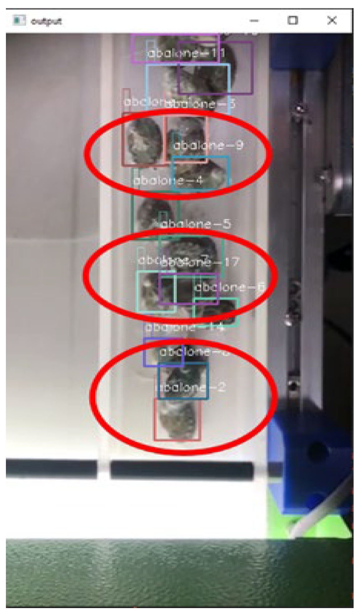
Using the test videos, multiple types of scenarios in which various abalones in the test videos were occluded were tested to ensure that the target tracking and counting method could operate stably. The detection of the occluded abalones is shown in Figure 9c.
To verify whether the proposed model in this study is effective, the abalone counting results of the proposed are compared with those of OpenCV detection with tracking and counting [43] and Blob detection tracking [47]. The length of test videos varied from 16 to 36 s. The actual number of abalones is counted manually from each video to compare the results presented by the models. The experimental results comparison are listed in Table 3.
The test results show that it takes an average of 30 fps to count the abalones per image. It can be observed from Table 3 that the YOLOv3 combined with DeepSORT counting model proposed in this article has great potential compared to OpenCV detection with tracking and counting and Blob detection tracking. The best accuracy with test video data is the accuracies of 94.4%. Due to the slow-motion effect in the video data, the third video give low performance as 64% of accuracy. Compared to the OpenCV detection with tracking and counting and Blob detection tracking, the results of YOLOv3 regarding object counting, the video monitoring accuracy rate of object tracking is improved. This study also considers that video data collection should be consistent since, with regard to the tested data, some of the video data have a slow-motion effect during collection. This makes it difficult to detect abalones owing to the inconsistency in video speed, which affects the maximum accuracy rate and abalone counting rate.
6. Conclusions and Future Work
This study presents a practical methodology for abalone counting using YOLOv3 and DeepSORT. The core components of the abalone counting methodology are the detection of abalones, tracking of abalones on the conveyor belt, and counting of moving abalones. Combined with the DeepSORT framework, YOLOv3 shows promising results in detecting and counting abalones.
The counting accuracy obtained by the proposed method is as high as 94%. However, it also exhibits a limitation in the slow-motion effect in the video sequence. In agreement with Park et al. [3], who used the LabVIEW machine vision approach in a conveyor belt for counting abalones, the proposed methodology provides a significant improvement in the collection of data, for instance, by positioning a camera on a fixed position where video data can be collected consistently.
Using the proposed methodology, the costs and time for counting abalones in the marine industry can be reduced, which will increase benefits and competitiveness. The proposed methodology can also be applied to similar industries.
Despite the promising performance of the proposed methodology, more work remains, such as improvement in the detection of entangled abalones, flexible adaptation to video quality in detection, and improvement in calculation speed.
Author Contributions
D.K.: writing, review, and editing of original draft; data analysis; data gathering; conceptualization. J.-H.S.: project administration; conceptualization; writing, review, and editing; supervision; funding acquisition. All authors have read and agreed to the published version of the manuscript.
Funding
This study was supported by a research fund from Chosun University (2020).
Data Availability Statement
Not applicable.
Acknowledgments
We gratefully acknowledge the Internal Research Fund of Chosun University (2020).
Conflicts of Interest
The authors declare no conflict of interest.
References
- Chen, L.; Ryan, J.C. Abalone in Diasporic Chinese Culture: The Transformation of Biocultural Traditions through Engagement with the Western Australian Environment. Heritage 2018, 1, 122–141. [Google Scholar] [CrossRef] [Green Version]
- Hadijah, H.; Mardiana, M.; Indrawati, E.; Budi, S.; Zainuddin, Z. The use of artificial feed in Haliotis squamata farming in submerged cage culture system at Lae-Lae island, Makassar. Rev. Ambiente Água 2021, 16. [Google Scholar] [CrossRef]
- Park, K.-M.; Ahn, B.-W.; Park, Y.-S.; Bae, C.-O. A Study on Abalone Young Shells Counting System using Machine Vision. J. Korean Soc. Mar. Environ. Saf. 2017, 23, 415–420. [Google Scholar] [CrossRef]
- Mathias, A.; Dhanalakshmi, S.; Kumar, R. Occlusion aware underwater object tracking using hybrid adaptive deep SORT -YOLOv3 approach. Multimedia Tools Appl. 2022, 81, 44109–44121. [Google Scholar] [CrossRef]
- Wang, Y.-Q. An Analysis of the Viola-Jones Face Detection Algorithm. Image Process. Online 2014, 4, 128–148. [Google Scholar] [CrossRef]
- Lee, K.L.; Mokji, M.M. Automatic target detection in GPR images using Histogram of Oriented Gradients (HOG). In Proceedings of the 2014 2nd International Conference on Electronic Design (ICED), Penang, Malaysia, 9–21 August 2014; pp. 181–186. [Google Scholar]
- Garay, J.R.; Kofuji, S.T.; Tiba, T. Overview of a system AMR based in computational Vision and Wireless sensor network. In Proceedings of the 2009 IEEE Latin-American Conference on Communications, Medellin, Columbia, 10–11 September 2009; pp. 1–5. [Google Scholar]
- Russakovsky, O.; Deng, J.; Su, H.; Krause, J.; Satheesh, S.; Ma, S.; Huang, Z.; Karpathy, A.; Khosla, A.; Bernstein, M.; et al. Imagenet large scale visual recognition challenge. Int. J. Comput. Vis. 2015, 115, 211–252. [Google Scholar] [CrossRef]
- Côté-Allard, U.; Fall, C.L.; Campeau-Lecours, A.; Gosselin, C.; Laviolette, F.; Gosselin, B. Transfer learning for sEMG hand gestures recognition using convolutional neural networks. In Proceedings of the 2017 IEEE International Conference on Systems, Man, and Cybernetics (SMC), Banff, AB, Canada, 5–8 October 2017; pp. 1663–1668. [Google Scholar]
- Wang, J.; Chen, K.; Yang, S.; Loy, C.C.; Lin, D. Region proposal by guided anchoring. In Proceedings of the IEEE/CVF Conference on Computer Vision and Pattern Recognition 2019, Long Beach, CA, USA, 15–20 June 2019; pp. 2965–2974. [Google Scholar]
- Kapsalas, P.; Rapantzikos, K.; Sofou, A.; Avrithis, Y. Regions of interest for accurate object detection. In Proceedings of the 2008 International Workshop on Content-Based Multimedia Indexing, London, UK, 18–20 June 2008; pp. 147–154. [Google Scholar]
- Wei, B.; Hao, K.; Tang, X.; Ren, L. Fabric defect detection based on faster RCNN. In Artificial Intelligence on Fashion and Textiles, Proceedings of the Artificial Intelligence on Fashion and Textiles (AIFT) Conference 2018, Hong Kong, 3–6 July 2018; Springer: Berlin/Heidelberg, Germany; pp. 45–51. [Google Scholar]
- Li, J.; Hou, Q.; Xing, J.; Ju, J. SSD object detection model based on multi-frequency feature theory. IEEE Access 2020, 8, 82294–82305. [Google Scholar] [CrossRef]
- Redmon, J.; Divvala, S.; Girshick, R.; Farhadi, A. You only look once: Unified, real-time object detection. In Proceedings of the IEEE Conference on Computer Vision and Pattern Recognition 2016, Las Vegas, NV, USA, 27–30 June 2016; pp. 779–788. [Google Scholar]
- Srivastava, S.; Divekar, A.V.; Anilkumar, C.; Naik, I.; Kulkarni, V.; Pattabiraman, V. Comparative analysis of deep learning image detection algorithms. J. Big Data 2021, 8, 66. [Google Scholar] [CrossRef]
- Zhong, J.; Li, M.; Qin, J.; Cui, Y.; Yang, K.; Zhang, H. Real-time marine animal detection using YOLO-based deep learning networks in the coral reef ecosystem. Int. Arch. Photogramm. Remote Sens. Spat. Inf. Sci. 2022, 46, 301–306. [Google Scholar] [CrossRef]
- Balakrishnan, B.; Chelliah, R.; Venkatesan, M.; Sah, C. Comparative Study on Various Architectures of Yolo Models Used in Object Recognition. In Proceedings of the 2022 International Conference on Computing, Communication, and Intelligent Systems (ICCCIS), Greater Noida, India, 4–5 November 2022; pp. 685–690. [Google Scholar]
- Xu, W.; Matzner, S. Underwater fish detection using deep learning for water power applications. In Proceedings of the 2018 International Conference on Computational Science and Computational Intelligence (CSCI), Las Vegas, NV, USA, 13–15 December 2018; pp. 313–318. [Google Scholar]
- Pedersen, M.; Bruslund Haurum, J.; Gade, R.; Moeslund, T.B. Detection of marine animals in a new underwater dataset with varying visibility. In Proceedings of the IEEE/CVF Conference on Computer Vision and Pattern Recognition Workshops, Long Beach, CA, USA, 16–17 June 2019; pp. 18–26. [Google Scholar]
- Shankar, R.; Muthulakshmi, M. Comparing YOLOV3, YOLOV5 & YOLOV7 Architectures for Underwater Marine Creatures Detection. In Proceedings of the 2023 International Conference on Computational Intelligence and Knowledge Economy (ICCIKE), Dubai, United Arab Emirates, 9–10 March 2023; pp. 25–30. [Google Scholar]
- Fu, C.-Y.; Liu, W.; Ranga, A.; Tyagi, A.; Berg, A.C. Dssd: Deconvolutional single shot detector. arXiv 2017, arXiv:1701.06659. [Google Scholar]
- Li, X.; Zhao, H.; Zhang, L. Recurrent retinanet: A video object detection model based on focal loss. In Neural Information Processing: Proceedings of the 25th International Conference, ICONIP 2018, Siem Reap, Cambodia, 13–16 December 2018, Proceedings, Part IV; Springer: Berlin/Heidelberg, Germany, 2018; pp. 499–508. [Google Scholar]
- Zhao, Q.; Sheng, T.; Wang, Y.; Tang, Z.; Chen, Y.; Cai, L.; Ling, H. M2det: A single-shot object detector based on multi-level feature pyramid network. In Proceedings of the AAAI Conference on Artificial Intelligence, Honolulu, HI, USA, 27 January–1 February 2019; Volume 33, pp. 9259–9266. [Google Scholar]
- Zhang, S.; Wen, L.; Lei, Z.; Li, S.Z. RefineDet++: Single-shot refinement neural network for object detection. IEEE Trans. Circuits Syst. Video Technol. 2020, 31, 674–687. [Google Scholar] [CrossRef]
- Redmon, J.; Farhadi, A. Yolov3: An incremental improvement. arXiv 2018, arXiv:1804.02767. [Google Scholar]
- Tseng, C.-H.; Kuo, Y.-F. Detecting and counting harvested fish and identifying fish types in electronic monitoring system videos using deep convolutional neural networks. ICES J. Mar. Sci. 2020, 77, 1367–1378. [Google Scholar] [CrossRef]
- French, G.; Fisher, M.; Mackiewicz, M.; Needle, C. Convolutional neural networks for counting fish in fisheries surveillance video. In Proceedings of the Machine Vision of Animals and their Behaviour (MVAB), Swansea, UK, 10 September 2015; BMVA Press: Durham, UK, 2015. [Google Scholar]
- Klapp, I.; Arad, O.; Rosenfeld, L.; Barki, A.; Shaked, B.; Zion, B. Ornamental fish counting by non-imaging optical system for real-time applications. Comput. Electron. Agric. 2018, 153, 126–133. [Google Scholar] [CrossRef]
- Du, J. Understanding of object detection based on CNN family and YOLO. J. Phys. Conf. Ser. 2018, 1004, 012029. [Google Scholar] [CrossRef]
- Al-Ariny, Z.; Abdelwahab, M.A.; Fakhry, M.; Hasaneen, E.-S. An efficient vehicle counting method using mask r-cnn. In Proceedings of the 2020 International Conference on Innovative Trends in Communication and Computer Engineering (ITCE), Aswan, Egypt, 8–9 February 2020; pp. 232–237. [Google Scholar]
- Hardjono, B.; Tjahyadi, H.; Rhizma, M.G.; Widjaja, A.E.; Kondorura, R.; Halim, A.M. Vehicle counting quantitative comparison using background subtraction, viola jones and deep learning methods. In Proceedings of the 2018 IEEE 9th Annual Information Technology, Electronics and Mobile Communication Conference (IEMCON), Vancouver, BC, Canada, 1–3 November 2018; pp. 556–562. [Google Scholar]
- Hung, G.L.; Sahimi, M.S.B.; Samma, H.; Almohamad, T.A.; Lahasan, B. Faster R-CNN deep learning model for pedestrian detection from drone images. SN Comput. Sci. 2020, 1, 116. [Google Scholar] [CrossRef] [Green Version]
- Asha, C.S.; Narasimhadhan, A.V. Vehicle counting for traffic management system using YOLO and correlation filter. In Proceedings of the 2018 IEEE International Conference on Electronics, Computing and Communication Technologies (CONECCT), Bangalore, India, 16–17 March 2018; pp. 1–6. [Google Scholar]
- Forero, A.; Calderon, F. Vehicle and pedestrian video-tracking with classification based on deep convolutional neural networks. In Proceedings of the 2019 XXII Symposium on Image, Signal Processing and Artificial Vision (STSIVA), Bucaramanga, Colombia, 24–26 April 2019; pp. 1–5. [Google Scholar]
- Mariam, K. Smart Annotation Approaches for Medical Imaging. Ph.D. Thesis, National University of Sciences and Technology, Islamabad, Pakistan, 2020. [Google Scholar]
- Mantiuk, R.K.; Hammou, D.; Hanji, P. HDR-VDP-3: A multi-metric for predicting image differences, quality and contrast distortions in high dynamic range and regular content. arXiv 2023, arXiv:2304.13625. [Google Scholar]
- Tabassum, S.; Ullah, S.; Al-Nur, N.H.; Shatabda, S. Poribohon-BD: Bangladeshi local vehicle image dataset with annotation for classification. Data Brief 2020, 33, 106465. [Google Scholar] [CrossRef]
- Muri, K.K.; Arne, W.; Knutsen, S.T.; Halvorsen, K.T.; Kleiven, A.R.; Lei, J.; Goodwin, M. Temperate fish detection and classification: A deep learning based approach. Appl. Intell. 2022, 52, 6988–7001. [Google Scholar]
- Girshick, R. Fast r-cnn. In Proceedings of the IEEE International Conference on Computer Vision 2015, Santiago, Chile, 7–13 December 2015; pp. 1440–1448. [Google Scholar]
- Gupta, P.; Gupta, S. Deep Learning in Medical Image Classification and Object Detection: A Survey. Int. J. Image Process. Pattern Recognit. 2022, 8, 1–15. [Google Scholar] [CrossRef]
- Su, H.; Jung, C. Perceptual enhancement of low light images based on two-step noise suppression. IEEE Access 2018, 6, 7005–7018. [Google Scholar] [CrossRef]
- Redmon, J.; Farhadi, A. YOLO9000: Better, faster, stronger. In Proceedings of the IEEE Conference on Computer Vision and Pattern Recognition 2017, Honolulu, HI, USA, 21–26 July 2017; pp. 7263–7271. [Google Scholar]
- Dadhich, A. Practical Computer Vision: Extract Insightful Information from Images Using TensorFlow, Keras, and OpenCV; Packt Publishing Ltd.: Birmingham, UK, 2018. [Google Scholar]
- Ma, H.; Liu, Y.; Ren, Y.; Yu, J. Detection of collapsed buildings in post-earthquake remote sensing images based on the improved YOLOv3. Remote Sens. 2019, 12, 44. [Google Scholar] [CrossRef] [Green Version]
- Rezatofighi, H.; Tsoi, N.; Gwak, J.; Sadeghian, A.; Reid, I.; Savarese, S. Generalized intersection over union: A metric and a loss for bounding box regression. In Proceedings of the IEEE/CVF Conference on Computer Vision and Pattern Recognition 2019, Long Beach, CA, USA, 15–20 June 2019; pp. 658–666. [Google Scholar]
- Cui, M.; Liu, H.; Liu, W.; Qin, Y. An adaptive unscented kalman filter-based controller for simultaneous obstacle avoidance and tracking of wheeled mobile robots with unknown slipping parameters. J. Intell. Robot. Syst. 2018, 92, 489–504. [Google Scholar] [CrossRef]
- Yusuf, M.D.; Kusumanto, R.D.; Oktarina, Y.; Dewi, T.; Risma, P. Blob analysis for fruit recognition and detection. Comput. Eng. Appl. J. 2018, 7, 23–32. [Google Scholar] [CrossRef]
Figure 1.
Abalone counting machine using conveyor belt.

Figure 2.
Entangled abalones on the conveyor belt.

Figure 3.
Overall architecture of abalone counting method.

Figure 4.
An example of Abalones annotated in (a) with bounding boxes using the LabelImg tool. (b) Example of a frame in the video data.
Figure 4.
An example of Abalones annotated in (a) with bounding boxes using the LabelImg tool. (b) Example of a frame in the video data.

Figure 5.
Darknet-53 convolutional network used by YOLOv3 to perform abalone detection.

Figure 6.
Applied general YOLOv3 framework.

Figure 7.
Training performance of YOLOv3 weights.

Figure 8.
Images from the test dataset showing the detection performance.

Figure 9.
Tracking of abalone in video: (a) Consistent tracking of abalone. (b) Tracking during occlusion and overlapping. (c) Sample frames from the video data showing frames per second, current count, total count, and two green lines (region where if the abalone passes it will be counted).
Figure 9.
Tracking of abalone in video: (a) Consistent tracking of abalone. (b) Tracking during occlusion and overlapping. (c) Sample frames from the video data showing frames per second, current count, total count, and two green lines (region where if the abalone passes it will be counted).


Table 1.
Comparison of previous works related to marine counting with machine and object counting with deep learning.
Table 1.
Comparison of previous works related to marine counting with machine and object counting with deep learning.
| Author | Used Model | Feature | Others | |||||
|---|---|---|---|---|---|---|---|---|
| D1 | D2 | D3 | D4 | D5 | D6 | |||
| Park et al. [3] | LabVIEW Machine vision in conveyor system | √ | √ | √ | ||||
| Garay et al. [7] | AMR system based | √ | ||||||
| Côté-Allard et al. [9] | CNN Model | √ | √ | √ | Hand gestures detection | |||
| Balakrishnan et al. [17] | YOLOv5, YOLOv3, Tiny YOLO and ResNet | √ | √ | Object recognition | ||||
| Shankar et al. [20] | YOLOv3. YOLOv5 and YOLOv7 | √ | √ | Fish identification | ||||
| Klapp et al. [28] | Hybrid non-imaging optics and an image processing scheme | √ | √ | √ | √ | Low signal-to-noise caused by water fluctuation and Fish size. | ||
| Garay et al. [7] | AMR system based | √ | ||||||
| Klapp et al. [28] | Hybrid non-imaging optics and an image processing scheme | √ | √ | √ | √ | Low signal-to-noise caused by water fluctuation and fish size | ||
| Hardjono et al. [31] | Viola Jones with background subtraction method | √ | √ | √ | √ | Background subtraction in images. | ||
| Hung et al. [32] | AlexNet model with multiple layers and edge boxes | √ | √ | √ | Δ | |||
| Asha et al. [33] | YOLO and correlation filter | √ | √ | √ | Real-time processing on edge devises such as Jetson Nano and Raspberry Pi | |||
| Forero and Calderon et al. [34] | YOLO with Tracking of Region Of Interest (ROI) | √ | √ | √ | √ | |||
| Our model | YOLOv3-TensorFlow | √ | √ | √ | √ | √ | √ | |
D1 Occlusion; D2 Detection; D3 Low resolution in images; D4 Tracking; D5 Count Errors; D6 Need for real-time application; √ Considered factors; Δ Need for large datasets.
Table 2.
YOLO format of annotated abalone in sample frame.
| Abalone (Class) | Height | Width | x | y |
|---|---|---|---|---|
| 15 | 0.504950 | 0.729167 | 0.128713 | 0.030556 |
| 15 | 0.512376 | 0.683333 | 0.123762 | 0.058333 |
| 15 | 0.538366 | 0.639583 | 0.111386 | 0.029167 |
| 15 | 0.623762 | 0.043750 | 0.133663 | 0.084722 |
Table 3.
Comparison of experimental results of YOLOv3-TensorFlow and DeepSORT, OpenCV detection tracking and counting and Blob detection tracking and counting.
Table 3.
Comparison of experimental results of YOLOv3-TensorFlow and DeepSORT, OpenCV detection tracking and counting and Blob detection tracking and counting.
| Model | Actual Number of Abalone | Counted Number by Model | Accuracy (%) |
|---|---|---|---|
| YOLOv3-TensorFlow and DeepSORT (proposed model) | 29 | 25 | 86.2 |
| 36 | 34 | 94.4 | |
| 25 | 16 | 64.0 | |
| 32 | 29 | 90.6 | |
| OpenCV detection tracking and counting | 29 | 20 | 68.9 |
| 36 | 25 | 69.4 | |
| 25 | 18 | 72.0 | |
| 32 | 20 | 62.5 | |
| Blob detection tracking and counting | 29 | 25 | 86.2 |
| 36 | 27 | 75.0 | |
| 25 | 20 | 80.0 | |
| 32 | 24 | 75.0 |
Disclaimer/Publisher’s Note: The statements, opinions and data contained in all publications are solely those of the individual author(s) and contributor(s) and not of MDPI and/or the editor(s). MDPI and/or the editor(s) disclaim responsibility for any injury to people or property resulting from any ideas, methods, instructions or products referred to in the content. |
© 2023 by the authors. Licensee MDPI, Basel, Switzerland. This article is an open access article distributed under the terms and conditions of the Creative Commons Attribution (CC BY) license (https://creativecommons.org/licenses/by/4.0/).
Share and Cite
MDPI and ACS Style
Kibet, D.; Shin, J.-H. Counting Abalone with High Precision Using YOLOv3 and DeepSORT. Processes 2023, 11, 2351. https://doi.org/10.3390/pr11082351
AMA Style
Kibet D, Shin J-H. Counting Abalone with High Precision Using YOLOv3 and DeepSORT. Processes. 2023; 11(8):2351. https://doi.org/10.3390/pr11082351
Chicago/Turabian StyleKibet, Duncan, and Jong-Ho Shin. 2023. "Counting Abalone with High Precision Using YOLOv3 and DeepSORT" Processes 11, no. 8: 2351. https://doi.org/10.3390/pr11082351
Note that from the first issue of 2016, this journal uses article numbers instead of page numbers. See further details here.