Life Cycle Cost Analysis of Pumping System through Machine Learning and Hidden Markov Model

Abstract

The pumping system is a critical component in various industries and consumes 20% of the world’s energy demand, with 25–50% of that energy used in industrial operations. The primary goal for users of pumping systems is to minimise maintenance costs and energy consumption. Life cycle cost (LCC) analysis is a valuable tool for achieving this goal while improving energy efficiency and minimising waste. This paper aims to compare the LCC of pumping systems in both healthy and faulty conditions at different flow rates, and to determine the best AI-based machine learning algorithm for minimising costs after fault detection. The novelty of this research is that it will evaluate the performance of different machine learning algorithms, such as the hybrid model support vector machine (SVM) and the hidden Markov model (HMM), based on prediction speed, training time, and accuracy rate. The results of the study indicate that the hybrid SVM-HMM model can predict faults in the early stages more effectively than other algorithms, leading to significant reductions in energy costs.

1. Introduction

Various industries worldwide depend on pumping systems for their daily operations. Optimising a pump is challenging across multiple application areas, like irrigation, water supply for the domestic sector, air conditioning systems, refrigeration, and the oil and gas industries, etc. [1]. In the world of pumps, two types of horizontal end suction centrifugal pumps are more widely used than all the others. They are the ANSI pumps designed and built to the American National Standards Institute standards and the API pump that meets the American Petroleum Institute standard 610 requirements for general refinery service. In order to handle high temperature and pressure applications of a more aggressive character, the API pump is the only option for the oil refinery business. Information on maintenance, failure, and repair times is provided for both pumps. This information has been used to demonstrate how precise predictions for life cycle costs for the pumps used in the hydrocarbon processing businesses may be made.

There is additional discussion of the fundamental ideas of LCC and its uses. In terms of global pumps, there is a need to apply LCC methodology to pumps, considering the stages of an LCC analysis, the need to identify the significant cost drivers, and the advantages of performing an LCC study. When the speed of the motor fluctuates in applications requiring variable torque, such as pumps, the torque produced by the pump likewise varies appropriately. An adaptive neuro-fuzzy inference system (ANFIS) is used in conjunction with DTC to lessen torque sags and enhance the reactivity of the control algorithm. The suggested ANFIS-based DTC has greatly reduced flux, torque, and stator current ripples compared to the conventional DTC and the fuzzy logic-based DTC. The suggested ANFIS-DTC results are verified using MATLAB simulations, and the system’s performance is determined to be good when evaluated at various rotational speeds. For the PMSM to drive centrifugal pumps, a new speed control based on adaptive neuro-fuzzy direct torque control (ANFIS-DTC) has been proposed in the research [2]. Through the Matlab Simulink environment, the performance characteristics of the conventional DTC, DTC with fuzzy logic control, and DTC with ANFIS are compared in terms of stator current, electromagnetic torque, stator flux, rotor speed, and pump output pressure. Compared to traditional DTC and DTC with fuzzy logic control, the suggested ANFIS-DTC controller displays satisfactory results in removing overshoot and ripples in torque, flux, and speed.

Some statistical measurements of the mean time between failures are also provided. For pumping systems, the Hydraulic Institute presented a life cycle cost model. Initial costs, installation and commissioning expenses, energy costs, operational costs, maintenance and repair costs, downtime costs, environmental costs, and decommissioning and disposal costs are all considered in the model. An example has been used to show how to apply the methodology. The guidelines developed by Euro-pumps to assist users, consultants, and design engineers in optimising pumping systems with regard to the whole life cost were presented in the research, along with an explanation of the significance of life cycle costs. The optimal operation aims to save electricity expenses, consume maximum energy, reduce water leakage, prevent wear and tear, etc. [3]. Various optimisation algorithms are helpful for reducing electricity expenses and saving consumption of energy, such as the heuristic algorithm [4], PSO [5], ant colony, genetic algorithm [6], etc. However, if the system requires transient changes, CNN model [7] is required to optimise the system. Due to the extreme progress of technology, the costs of variable speed drives have significantly decreased, which is helpful for the pumps used in building conditioning systems. Control and optimisation of variable speed pump operation is a challenging issue. Control engineers have a great responsibility to control the robustness of the pump, improve the operating efficiency, prolong the service life, etc. [8]. An energy-efficient pump scheduling strategy can reduce maintenance and operating costs. In this way, it is possible to reduce CO₂ emissions [9]. Various researchers have conducted extensive studies on pump optimisation and scheduling. Mixed integer nonlinear programming has been used to solve the structural optimisation problem, as the problem is not convex. A binary separable program method has been developed for the optimum global system [10]. The method provides the best configuration of the pump series. The optimal pump scheduling algorithms have been introduced for the water distribution system. An energy-efficient pump scheduling strategy has enormous potential to significantly reduce pump systems’ operational and maintenance costs [11]. For instance, up to 90% of the electricity used in the water industry is consumed by pumps. Purchasing decisions for a pump and the associated system components are often based on the lowest offer rather than considering the system’s cost over its life cycle [12,13,14,15].

To achieve the lowest energy usage and cost, managers must carefully match these interdependent parameters and ensure they are maintained during working conditions [16]. A pumping system typically lasts 15 to 20 years. Some costs will be incurred initially, while others may appear at various points throughout the existence of the multiple options under consideration. Therefore, determining a current or discounted value of the LCC is conceivable and possibly even necessary to properly evaluate the various alternatives [17].

The LCC procedure forecasts the most economical option; it does not assure a certain result, but it enables the plant manager or designer to assess several solutions while considering the limitations of the data at hand [18,19,20], as in the following Equation (1):

$$\mathbf{L}\mathbf{C}\mathbf{C}={\mathit{C}}_{\mathit{i}\mathit{c}}+{\mathit{C}}_{\mathit{i}\mathit{n}}+{\mathit{C}}_{\mathit{e}}+{\mathit{C}}_0+{\mathit{C}}_{\mathit{m}}+{\mathit{C}}_{\mathit{S}}+{\mathit{C}}_{\mathit{e}\mathit{n}\mathit{v}}+{\mathit{C}}_{\mathit{d}}$$

(1)

where LCC is life cycle cost, ${\mathit{C}}_{\mathit{i}\mathit{c}}$ is initial cost means purchase cost, ${\mathit{C}}_{\mathit{e}}$ is energy cost, ${\mathit{C}}_0$ is operation cost, ${\mathit{C}}_{\mathit{m}}$ is maintenance and repair cost, ${\mathit{C}}_{\mathit{S}}$ is downtime cost, ${\mathit{C}}_{\mathit{e}\mathit{n}\mathit{v}}$ is an environmental cost, ${\mathit{C}}_{\mathit{i}\mathit{n}}$ is commissioning and installation cost, and ${\mathit{C}}_{\mathit{d}}$ is disposal cost. Figure 1 shows the various parts of the costs, which are the combinations of the LCC.

The following consecutive sections will highlight the importance of life cycle cost, the application of the hidden Markov model [21,22] for LCC prediction, the application of HMM and machine learning analysis, the proposed method, the results and analysis, and the conclusion.

2. Background of Related Work

There is a significant body of research on pumping systems’ life cycle cost analysis (LCCA). This section focuses on the background research on existing works of LCC analysis of the pumping system. Three distinct pumps have undergone an LCC analysis using a technique based on dependability and maintainability principles, and the results have been compared. Two pumps have been chosen from the literature for analysis, and the information therein is used. The third pump is chosen from a reputable Indian pump manufacturer, and the necessary information is acquired directly from the supplier. The idea of the predicted number of failures in a particular time interval has been used to model the maintenance and repair costs [23]. A methodology for calculating the net present value (NPV), lifetime costs (LCC), energy use, and greenhouse gas emissions related to a water distribution system (WDS) pump using a process-based life cycle assessment (LCA) and an economic input-output LCA (EIO-LCA) model has been described in the research. The methodology takes into account the stages of production, usage, and end-of-life (EOL) disposal in addition to less common operations, such as discharge valve throttling, pump testing, deterioration, refurbishment, and variable speed pumping. A case study presents the technique, evaluates the effects of various operating scenarios, and establishes the relative significance of various processes [24]. A study compares and contrasts decentralised greywater reuse systems’ life cycle costs and anticipated financial gains.

In comparison to the current centralised systems, the extra life cycle expenses and expected life cycle financial benefits of the groundwater pumping systems and on-site greywater reuse systems are assessed. Before the wastewater effluent is dumped into the environment, a sewer network gathers used water for treatment at a centralised wastewater treatment plant. Centralised systems refer to the traditional form of water delivery where one centralised treatment plant treats and distributes potable water to a large service area [25]. The optimal design and rehabilitation of a water distribution network are being provided using a new multiobjective formulation to minimise life cycle cost and maximise performance. The initial cost of the pipes, the cost of replacing old pipes with new ones, the cost of cleaning and lining existing pipes, the anticipated repair cost for pipe breaks, and the salvage value of the replaced pipes are all included in the life cycle cost. The resilience index has been modified for use in water distribution networks with multiple sources as the performance measure suggested in this study. In order to find a solution for the design and rehabilitation challenge, a new heuristic strategy is suggested [26]. In order to guarantee the excellent performance of chilled water pump systems and achieve the lowest annual total cost while taking input uncertainties and system reliability into account, this research proposed a reliable, optimal design method that is based on a reduced life-cycle cost. It is accomplished by optimising the number of chilled water pumps, overall pump flow capacity, and the pump pressure head [27].

The suggested approach is tested and shown using a case study. The amount of literature on the life cycle cost of wastewater treatment has significantly increased over the past two decades. The employment of several frameworks and approaches was caused by the lack of a generally accepted life cycle costing methodology. Over the past ten years, a progressive transition from conventional to environmental and societal life cycle costing has been observed. Techniques and approaches for conducting life cycle cost analysis are also changing.

Nevertheless, there is still a need for a thorough, systematic assessment of life cycle costing techniques and methodologies in wastewater treatment. A thorough and systematic evaluation offers the chance to track recent advancements in the subject and pinpoint areas that require additional study [28]. In order to effectively assess the long-term treatment performance and cost under influent fluctuations, this study uses artificial neural networks (ANNs) as surrogate models for water resource recovery facility (WRRF) models. A current facility that handles combined domestic and industrial wastewater served as the model for the five WRRFs. Even though the prediction performance (R-square) somewhat declines with increasing model complexity, the ANNs satisfactorily capture nonlinear biological processes for all five WRRFs. By using ANNs trained by simulation data from steady-state models to simulate long-term (10-year) performance with monthly influent fluctuations, the application of ANNs in WRRF models is expanded, and their effectiveness in removing phosphorus (P) and nitrogen (N) is expanded. Because enhanced biological phosphorus removal and recovery (EBPR) is more susceptible to influent characteristics altered by storm water inflow, EBPR-S has the greatest resistance. To create adequate working conditions, mine-dewatering techniques must be used to eliminate water flow into the mining area. One method of mine dewatering involves the use of pumps. Centrifugal and positive displacement pumps are primarily employed in mine dewatering operations. The primary goal of this project is to create a simple decision-support tool for choosing the most cost-effective pump type. The research approach employed in this study includes a literature review of the pump-type literature and case scenario data for economic analysis. Graphical user interfaces (GUI) were integrated into developing a decision support tool so that decision makers may choose which pump to utilise. Finally, case study data were used to test the program [29]. For condition-based maintenance (CBM) to increase the reliability and cost-effectiveness of maintenance, accurate remaining usable life (RUL) prediction of machines is crucial. In order to improve the precision of the RUL prediction of bearing failure, this paper suggests using artificial neural networks (ANN) [30].

The ANN model employs time and fitted measurements from its present and prior points as input, together with Weibull hazard rates for root mean square (RMS) and kurtosis. The output is chosen to be the normalised life percentage in the meantime. In doing so, reducing the degradation signal noise from target bearings and raising the prognosis system accuracy is possible. The feedforward neural network (FFNN) with the Levenberg–Marquardt training method is used for the ANN RUL prediction [31]. To reduce catastrophic failure events, the notion of remaining useful life (RUL) is used to predict the life span of components. It is essential to have a continuous monitoring system that records and identifies trends, as well as sources of component degradation prior to failure as customer demand for dynamically regulated systems increases. The goal of the early warning capacity is to identify, localise, and gauge the severity of defects using fault propagation and identified machine or component deterioration to forecast RUL. RUL is typically computed randomly from data on condition and health monitoring that is readily available. Remanufacturing engineers must consider a device’s RUL when deciding which parts should be removed from service for remanufacturing. The numerous approaches to forecasting a machine’s or component’s RUL are the focus of this review. Using case studies, some techniques for estimating RUL, including those for automotive components, rotating equipment, aviation engines, electro-hydraulic servo valves, electronic systems, low methane compressors, bearings, etc., are examined [32]. Further research has been carried out based on support vector regression analysis, XGboost, and PSO for pump performance curve analysis. The performance prediction model has been trained on 428 samples in total, while 107 samples are used to evaluate the model’s capacity to generalise, and 46 examples are used to confirm the model’s ability to predict outcomes [33]. Some research based on

Table 1. Various research based on LCC analysis.

Author	Research Technology	Aim of the Research	Research Outcome
Galagedarage Don, M., and Khan, F. [11]	Hidden Markov model–Bayesian networks	To predict and identify the faults	The suggested method adequately predicts all ten flaws and isolates eight of the ten defects found. The maximum acceptable noise levels for the various flaws were established, and the isolation accuracy changed depending on the noise level added to the testing data.
Hofmann, P., and Tashman, Z. [13]	Hidden Markov model	To detect the failure events	It is combined with a Markov mixed membership model (MMMM) and an observable Markov decision process (POMDP) for each asset to evaluate the trade-off between the risk of failure and prolonged operational hours to dynamically optimise the strategy for when and how to maintain the asset.
Waghmode, L.Y., et al. [23]	Economic input/output LCC model	To learn when the pump will end its useful life and how much energy the water distribution system uses	Refurbishing and variable speed pumping can improve a pump’s overall sustainability by reducing lifetime expenses, particularly in terms of energy use and GHG emissions.
Jayaram, N., and Srinivasan, K. [25]	Multiobjective formulation	To determine the optimal design and rehabilitation of water distribution network	As novel multiobjective formulations for the optimum network design and rehabilitation, the maximisation of the least modified resilience index and the minimisation of life cycle cost have been proposed. The adjusted resilience index measures the network’s ability to handle uncertainty.
Cheng, Q., et al. [26]	Robust optimal design	Calculating the uncertainties generates the cooling load distribution and hydraulic resistance distribution using Monte Carlo simulation	When uncertainties are taken into account, the annual average cooling load varies significantly. The design cooling capacity and chilled water flow will most likely be large if the design cooling capacity is designed based on the cooling load without considering uncertainties. For high accuracy and quick computing, the Markov method can be used to obtain the probability distribution of the system state.
Ilyas, M., et al. [27]	Various conventional approaches to LCC analysis	To find out the impact of LCC in wastewater treatment	The authors examined 66 studies on the LCCA of pumping systems and discovered that energy cost was the most significant factor in life cycle cost. They also found potential cost benefits from using variable speed drives and high-efficiency pumps.
Li, S., et al. [28]	Artificial neural network	Assessing water resource recovery facilities’ long-term treatment performance and nutrient removal costs under stochastic influence characteristics	Five different WRRF treatment options’ long-term nutrient removal efficacy and cost-effectiveness have been compared using a unique methodology. Using ANN models for long-term simulation can significantly reduce the computational load while maintaining acceptable accuracy, making it easier to couple complicated process models.
Aktaş, Ali Burak [29]	Decision support tool	Utilising LCC analysis, this evaluates centrifugal and positive displacement pumps in mine dewatering operations and creates a program as a decision assistance tool	Since LCC focuses on overall costs rather than the initial capital investment cost of the systems, it can be utilised as a decision-support tool. The total cost of the centrifugal pump is more than the positive displacement pump.
Saon, S., and Hiyama, T. [30]	Artificial neural network	Predicts the remaining useful life of rotary machine	CBM prioritises a machine’s precise RUL to boost dependability and reduce maintenance expenses. This research recommends utilising ANN to provide a more accurate estimate RUL of a bearing failure. In this case, the ANN model’s input is the Weibull hazard rates of RMS and kurtosis from the current and prior points. The output, which is the normalised life percentage, is also chosen.
Salunkhe, T., et al. [31]	Various conventional methods	To predict the remaining useful life of mechanical components	Model-based approaches are employed when there is a chance that the system could be mathematically modelled. When it is impossible to create a mathematical model of the system, data-driven approaches are applied.

describes various investigations into LCC analysis and RUL application in industrial sectors and their results.

3. Importance of Life Cycle Cost

If pumps are utilised for more than 2000 h annually, energy consumption, which is often one of the most significant cost components, may dominate the LCC. Information about the output pattern of the system is gathered to calculate energy consumption. If the output is continuous or nearly so, the calculation is straightforward. A time-based consumption pattern must be established if the production fluctuates over time [21,22,23,24,25,26,27,28,29]. Operating costs are the labour expenses related to running a pumping system. Depending on the complexity and duty of the system, these vary substantially. A pump must be efficiently and routinely serviced to obtain the best performance [34]. Unexpected downtime and lost production costs account for a sizeable portion of the total LCC and can have an impact comparable to those of energy and replacement part costs. Most of the time, the price to dispose of a pumping system will not change substantially based on its design [35]. A life cycle cost analysis (LCCA) is an economic evaluation method used to compare different alternatives over the life cycle of an asset. In the case of a pumping system, an LCCA would compare the costs of various pump systems over their expected lifespan, including initial purchase, maintenance, energy, and replacement costs. The application of artificial intelligence (AI) in pumps can significantly improve their energy efficiency, reduce maintenance costs, and prolong their lifespan. It is seen that with AI applications, most of the costs are reduced, and it becomes possible to save energy. Therefore, in the present research, machine learning-based AI technology has been implemented for a case study to analyse the LCC during the faulty condition of the pump.

There can be a distinction when a system includes disposal arrangements as a component of its operational arrangements. A total life cycle cost analysis (LCCA) is the methodology for evaluating bridge intervention solutions that are presented in the study [35,36]. Life cycle cost (LCC) analysis involves assessing the total cost of owning and operating a system or equipment throughout its life cycle, including acquisition, operation, maintenance, and disposal. Various types of research show in

Table 2. Various results based on LCC analysis.

LCC Analysis Components	Pumps in AI Application	Pumps without AI Application
Acquisition cost	Due to specialist pumps that are compatible with AI systems, there could be greater initial costs.	In AI applications, pumps are compared based on kind, capacity, and manufacturer.
Operation cost	Due to AI optimisation, there could be potential energy savings and lower operating expenses.	Due to a lack of AI optimisation, there will be greater energy consumption and possibly higher operating costs.
Maintenance cost	Due to AI-enabled proactive repairs and predictive maintenance, maintenance expenditures may be reduced.	Higher maintenance costs due to scheduled maintenance or reactive repairs without AI.
Efficiency and performance	Real-time optimisation and adaptive control have improved performance and efficiency.	Lower efficiency and suboptimal performance level.

that LCC analysis can be performed to compare the costs associated with using pumps in AI applications and without AI applications [37,38].

4. Proposed Method

The recent research is based on a VFD-based cascaded pump system with three pumps connected. The purpose of the research is to find out the impact of LCC analysis on the pumping system during a faulty condition, the remaining useful life of the pump after the fault, and, if an ML-based algorithm is used to detect the fault at an early stage, how the LCC cost can be reduced. The proposed study is divided into various steps.

Step 1: A case study has been analysed to create various faults in the pump to analyse the LCC cost.

Step 2: Find out the major fault among all kinds of faults in the pump; it is seen that a cavitation fault is the major fault in the pumping system in the present case study analysis.

Step 3: Apply various machine learning algorithms to predict the LCC cost analysis and the remaining useful life of the pump.

Step 4: Identify the remaining useful life of the pump. It is seen that the SVM and HMM hybrid method is more suitable for reducing the pump’s LCC cost than during a faulty condition. Then, the analysis was performed based on prediction speed, training time, and energy cost per hour for the SVM and HMM.

The data were collected during a healthy state and during three faulty conditions, including cavitation and water hammering. Then, after data collection, all the data were cleaned in Matlab software. The Matlab classifier learner tool extracted features and classified data successfully. Then, various ML algorithms were implemented to analyse which algorithm suits LCC pump analysis during faulty conditions. Furthermore, the pump’s remaining useful life has also been studied in the present research.

Figure 2 shows the steps of the process of ML algorithms.

5. Application of the Hidden Markov Model for LCC Prediction

The hidden Markov model (HMM), with its solid statistical foundation and efficient learning algorithm, enables learning to occur directly from raw sequence data. It supports variable-length inputs and consistently manages insertion and deletion penalties through locally learnable algorithms [39]. They are the sequence profiles with the widest range of generalisation. A few of the various tasks it is capable of include multiple alignments, data mining and categorisation, structural analysis, and pattern detection. But only each state and its accompanying objective function are necessary for HMM to function [40]. In the case of HMM, predicted function and target function do not match. In this situation, ML algorithms will take a long time to use with HMM. The accuracy rate of the expected function will be high, and, more accurately, the machine’s life cycle and the machine’s remaining useful life can be detected.

Markovian transition employs condition states (CSs) [41], forming a new deterioration matrix with transition probability for a new element. The hidden Markov model generally detects the machine’s health and useful life. The hidden Markov model determines unobservable hidden behaviour and remotely helps to access inaccessible electronic signals through observable signals [42]. For the purpose of water pumping in rural regions, several renewable energy resource–technology combinations have undergone a financial study and comparison. Options include dual-fuel IC engine pump sets powered by biogas, and producing gas, windmill pumps, and solar photovoltaic pumping systems.

The cost per unit volume of water pumped, the cost incurred per unit of useful hydraulic energy, and the present value of life cycle costs over a given period of time are the three figures of merit used to facilitate the comparison of the renewable options with conventional pumping systems, such as a diesel engine and electric motor pump sets. It has also been investigated how sensitive one of these figures of merit is to variations in the values of some of the input factors [43].

6. Application of HMM and Machine Learning for LCC Analysis

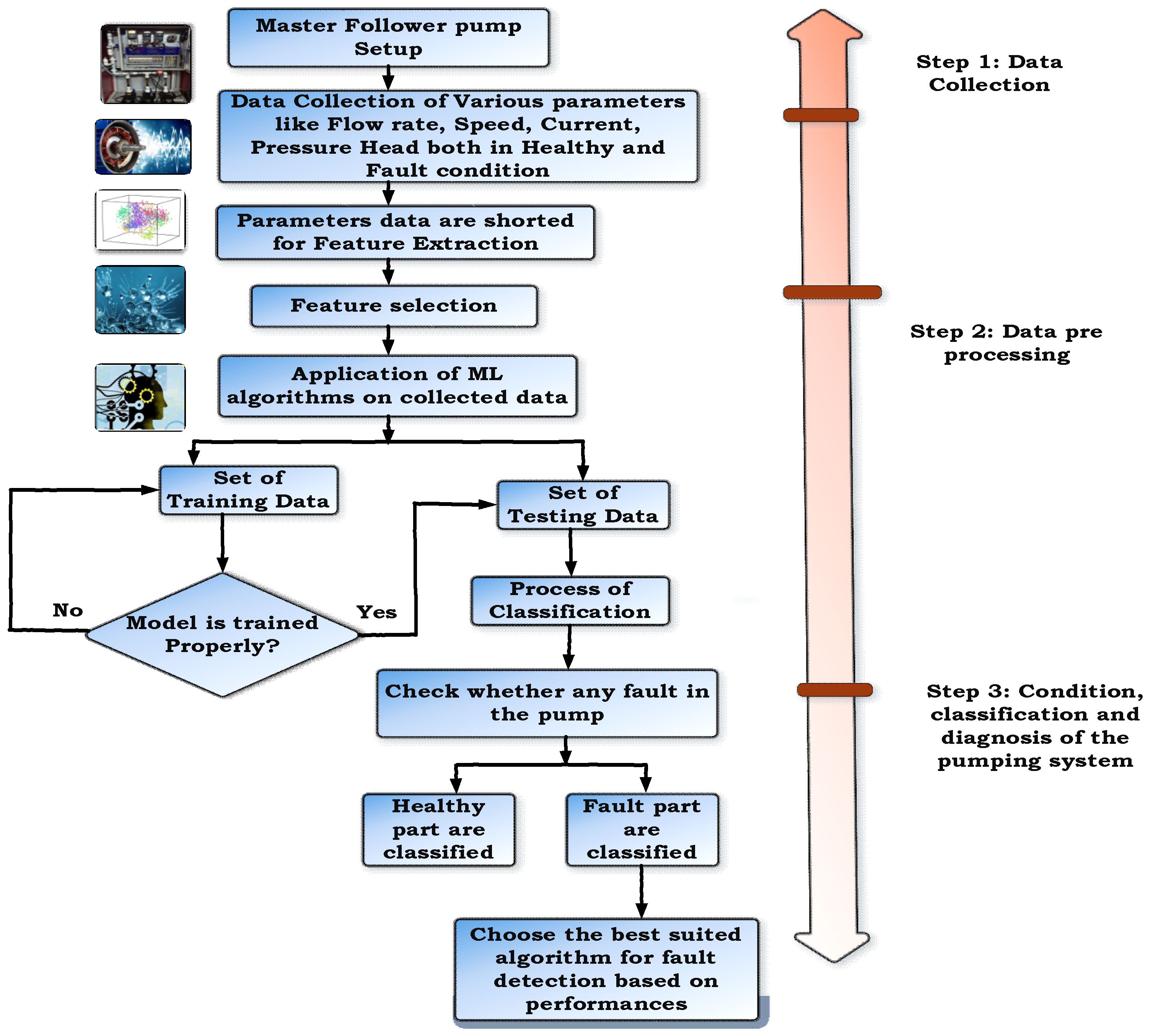
State transitions come in a variety of dialects. Each one represents the states, transitions, and events that can result in each transition. State transitions may also refer to conditions that govern whether a legal transition is permissible, and actions taken during a transition or upon entry into a new state. Because a state transition defines a finite-state automaton, the modelled object can only be in one state at a time. State transitions can be used to define a software module’s control structure or the modes of operation of large systems. To avoid the restrictions of HMM, the present study focuses on the hybrid technique where machine learning algorithms have been applied along with HMM. HMM identifies the machine’s state, and machine learning (ML) predicts the anomalies in the early stage. Massive tools for analysing complicated data produced by research into experimental and computational materials are provided by machine learning, in particular. Predictive maintenance’s main emphasis is on failure events. In order to predict future failures, it seems sensible to start by accumulating historical data on the machines’ performance and maintenance history. An essential indicator of equipment condition is usage history data. Since manufacturing equipment normally has an operational life of several years, historical data should be gathered far enough in the past to correctly depict the deteriorating processes of the equipment. The cost of breakdown includes not only the opportunity loss but also the machine’s fixed cost. Furthermore, production delays can result in penalties and lost orders. Other machines are also dependent on the failed machinery. A single breakdown can easily cost thousands of dollars. This loss will almost never be recovered. Failure probability can now be estimated using predictive models. This provides two abilities. The first is the ability to plan maintenance so that loss is minimised. Second, it makes it possible to improve inventory optimisation. Instead of stockpiling many spare parts, it is now possible to keep only those needed soon. ML can be used to help with the efforts mentioned earlier. The decision model created from the intrinsic facts then directs future activity. The performance of the system can be enhanced by these algorithms’ ability to identify and decide on optical communications. An average pumping system lasts 15 to 20 years. Some expenses will be incurred upfront, while others could arise at different times during the course of the life of the various solutions being considered [44,45]. This lifespan of the pump may reduce if any fault in the pumping system cannot be identified in the proper time. In that case, LCC costs also will be high. In this paper, through a case study, it is shown that if a fault happens, the cost will be high, and how that cost can be reduced by identifying the fault through ML and hidden Markov theory. The life cycle regression model has often been applied for prediction. SVM techniques are preferable to regression analysis in situations where fault classification is necessary and where it is necessary to distinguish between fault and no-fault locations with sparse data. The supervised learning machine includes SVM. It constructs a hyperplane or group of hyperplanes for the high infinite dimensional space used for classification and regression.

6.1. Application of Support Vector Machine for LCC Analysis

The idea of decision planes, which specify decision boundaries, serves as the foundation for support vector machines. A decision plane distinguishes between a group of items with various class affiliations. A primary classifier approach called a support vector machine distinguishes instances of distinct class labels using hyperplanes built in a multidimensional space. SVM, which permits both regression and classification tasks, can handle many continuous and categorical variables.

6.2. Application of SVM and HMM for Fault Analysis

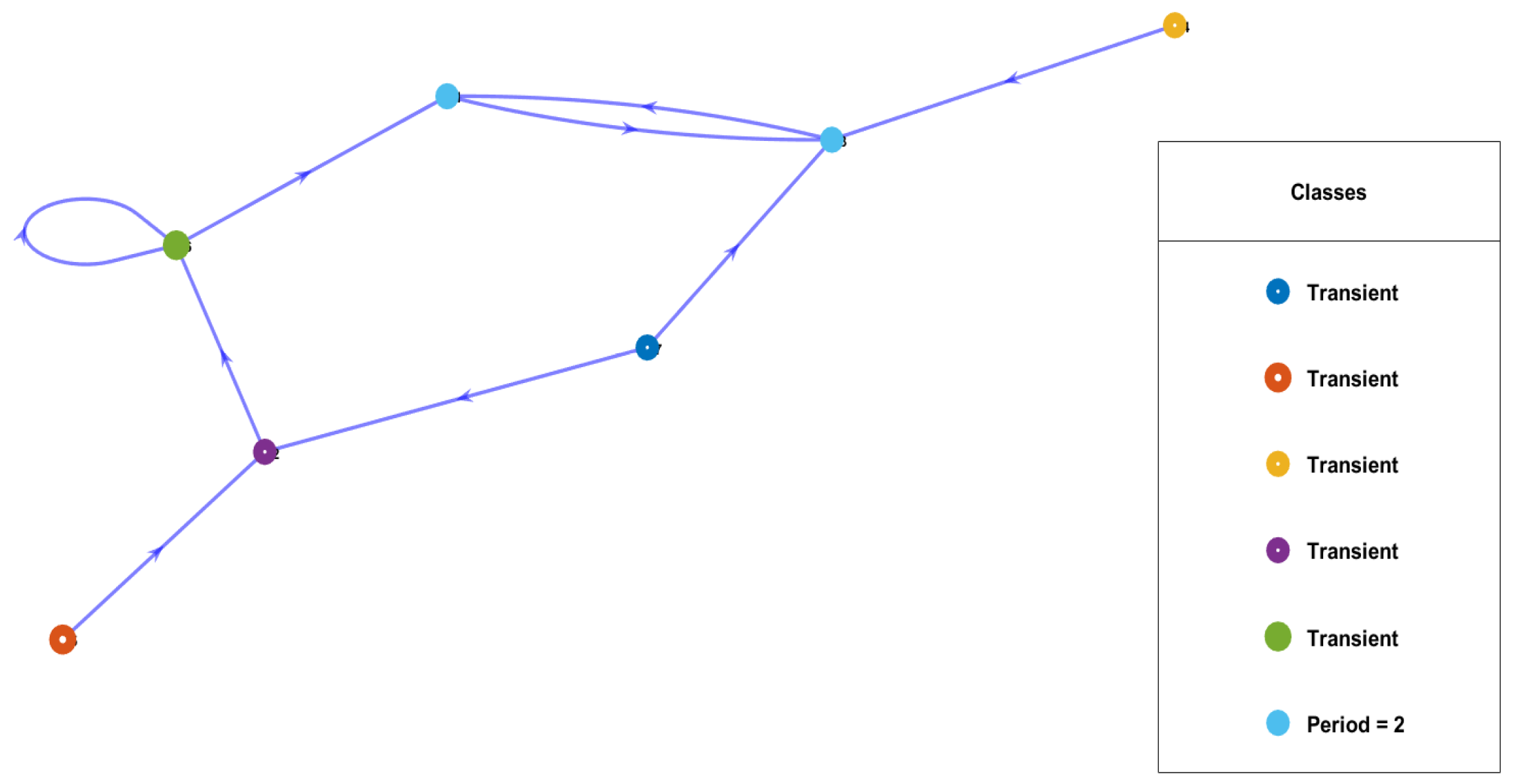
HMM will help to find the state of the data, and then, based on that prediction, the lifespan of the pump can be identified. If a sudden fault happens in the pumping system, the first work is to identify which part of the system has been affected. For this reason, two states have been chosen: a good state denoted by 0, and a warning state denoted by 1. HMM should analyse only the warning or fault state. If it is assumed at the beginning of the experiment that the pump is in good condition, then $X_0=0$, and the conversation rate matrix is shown as follows:

$$\Lambda =\left(\begin{array}{ccc}-({\lambda }_{01}+{\lambda }_{02})& {\lambda }_{01}& {\lambda }_{02}\\ 0& -{\lambda }_{12}& {\lambda }_{12}\\ 0& 0& 0\end{array}\right)$$

(2)

where ${\lambda }_{01}, {\lambda }_{02},{ \lambda }_{12}$ are the unknown parameters and should be estimated. Since the system deterioration occurs from state 0 to state 1, the probability of the faulty state is high. Before entering failure state 2, the fault in the system should be identified and rectified.

The SVM algorithm can intelligently extract equipment state characteristics from multiple indicators to determine whether the equipment fails. The critical advantage of SVM over conventional approaches is its ability to construct a precise mathematical model for fault diagnosis without having any prior knowledge of the internal relationships between the indicators. The model developed using the SVM algorithm is capable of detecting these inaccuracies. Here, the suggested technique takes advantage of hints to find enhanced accuracy. Here, indicator 1 is used as normal condition state, and indicators 2 to 5 are four different faulty condition states in the pumping system.

Figure 3 shows that historical data are gathered from time t − n to t, with the indication set at time t. A logical strategy is used to forecast the equipment state at time t. It is also used to predict when the equipment will break down. The physical data are measured using the indicators. The short-term tendency is then predictable, as their fluctuating tendency turns into a continuous curve. The indications on a piece of equipment will fluctuate more noticeably when it is about to fail. A pump’s remaining useful life (RUL) refers to how long it can operate effectively before it requires maintenance, repair, or replacement. Life cycle cost (LCC) analysis of a pump, on the other hand, is a method for comparing the total costs associated with the operation of the pump over its entire life cycle. The hybrid model aims to highlight their benefits and minimise their drawbacks. The one-to-rest approach of SVM was first dropped because of growing challenges in practical application. How to reduce the invalid outputs was the central area of concern. It is difficult to easily recognise the fault’s state when various faults occur in the pumping system at a time. In this research, vibration data have been collected in every fault case to analyse the fault state.

Along with that, the main parameters of pumping system i.e., flowrate and pressure value, were also collected for the analysis. Based on time, flow data have been collected. Now, based on the fault code, the output likelihood of HMM and SVM and condition states have been recognised. Here, data have been collected by creating a temporary fault in the pump by sudden valve closing and opening; for this reason, huge vibration and shock have been generated, and a loss of the bearing of the motor vibration has been created to check the bearing problem in the pump. The HMM plays a significant role. HMM has brought defect diagnosis and achieved considerable success. HMM is an excellent choice for modelling dynamic time series, particularly when the signal has a lot of information but is non-stationary, repeatable, and poorly reproducible. However, there are still a number of issues with the fault diagnosis utilising HMM. The user would benefit from the relative independence of the training of HMMs in different states, but the recognition accuracy would suffer. The disparity between various HMM outputs is not solely based on mathematics. Therefore, HMM is a beneficial classification tool for defect diagnosis, but its modelling skills are its best strength. A family of generalised linear classifiers includes the SVM. As an example, it concurrently minimises the empirical classification error and maximises the geometric margin when tackling the small sample, nonlinear, and high dimensional pattern recognition problems. Typically, SVM is used for binary classification. SVM uses two standard techniques to split a multiclass problem into numerous binary classification issues.

One-to-one is the first. Simply put, this method classifies the multiclass using n(n + 1)/2 SVMs, where n is the number of classes, and each SVM represents a hyperplane between the two classes. One-to-rest is the second strategy. This technique only requires n SVMs. A binary problem is present in the vectors of state1 and the other vectors while the SVM is being trained, such as the SVM of state1. Both approaches offer benefits and drawbacks that are unique to them. The hybrid model aims to highlight their benefits and minimise their drawbacks. The one-to-rest method of SVM initially suffers because of growing challenges in its practical application. How to reduce invalid outputs is the central area of concern. It is interesting to note that the output of the HMM related to the actual state was frequently the second or third largest as the mistake recognition started to appear.

Table 3. Fault codes for SVM and HMM for diagnosis.

Fault Code	No. of Samples	SVM and HMM		HMM
		Correct Samples	Correct Rate	Correct Samples	Correct Rate
110	250	250	100%	200	89%
101	250	250	100%	150	86%
11	250	200	98%	120	85%
1	250	180	95%	100	82%
10	250	150	92%	90	70%
100	250	100	90%	84	75%
0	250	90	90%	80	79%

shows model state conditions in different fault states. There are 250 samples carried out in each fault state. It is seen that instead of using only HMM, the hybrid model of SVM and HMM is more effective for correct fault state identification.

Figure 4 shows how the hybrid model SVM and HMM works after feature extraction from the raw data.

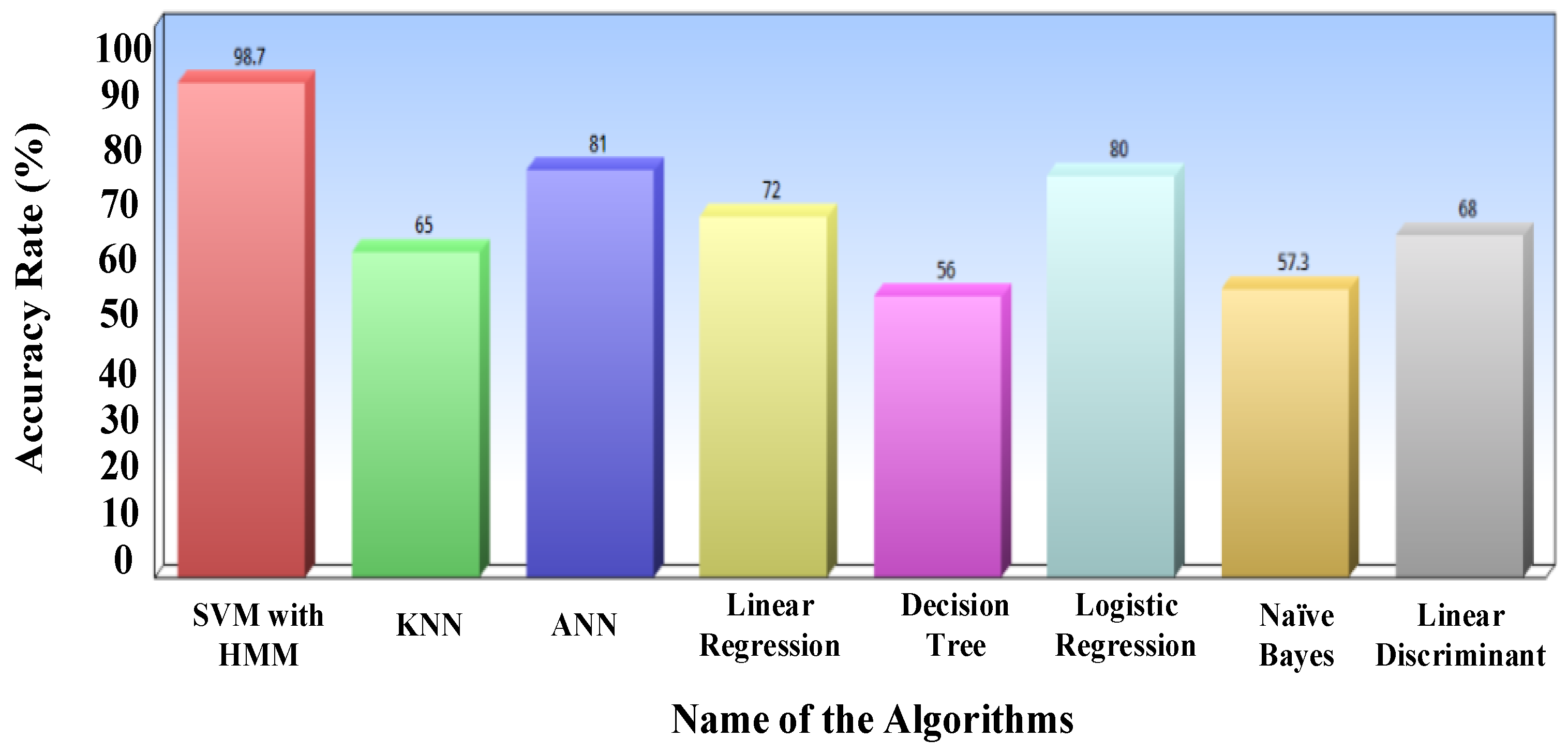
Figure 5 shows the recognition rate of SVM and HMM which will indicate the effect of the hybrid model. Due to active methods, SVMs could occasionally be high-speed machining independently further reinforced without concern of over-strengthening, which might affect other fault diagnostics.

There is a direct relationship between the RUL and LCC of a pump. The RUL provides critical input to the LCC analysis, as it determines the timing and cost of the pump’s maintenance, repair, or replacement. By estimating the RUL of the pump, it is possible to optimise the timing and cost of maintenance, repair, or replacement to minimise the overall LCC of the pump.

For example, if the RUL of a pump is estimated to be relatively short, it may be more cost-effective to perform maintenance that is more frequent or to make repairs to extend the pump’s operating life. On the other hand, if the RUL is estimated to be relatively long, it may be more cost-effective to continue operating the pump without any significant maintenance or repair until it reaches the end of its useful life, and then replace it with a new pump.

In addition to determining the timing and cost of maintenance, repair, or replacement, the RUL can also affect the energy consumption and efficiency of the pump. As the pump approaches the end of its useful life, it may become less efficient and consume more energy, which can increase the overall LCC of the pump.

Therefore, by estimating the RUL of a pump and incorporating it into the LCC analysis, it is possible to optimise the operating and maintenance strategies of the pump to minimise its overall life cycle cost. In the present research, after fault creation along with LCC analysis, it is possible to determine how much remaining useful life is pending for the pump system that has also been analysed to understand the other costing of the pump.

Figure 6 shows that in the 70 to 75 hours after a fault, the pump can give the best operating service, after which its working ability will start to reduce. Then, at 82 h, it will stop working. Based on that, the maintenance and other costs can be calculated, which will help to analyse the overall LCC cost.

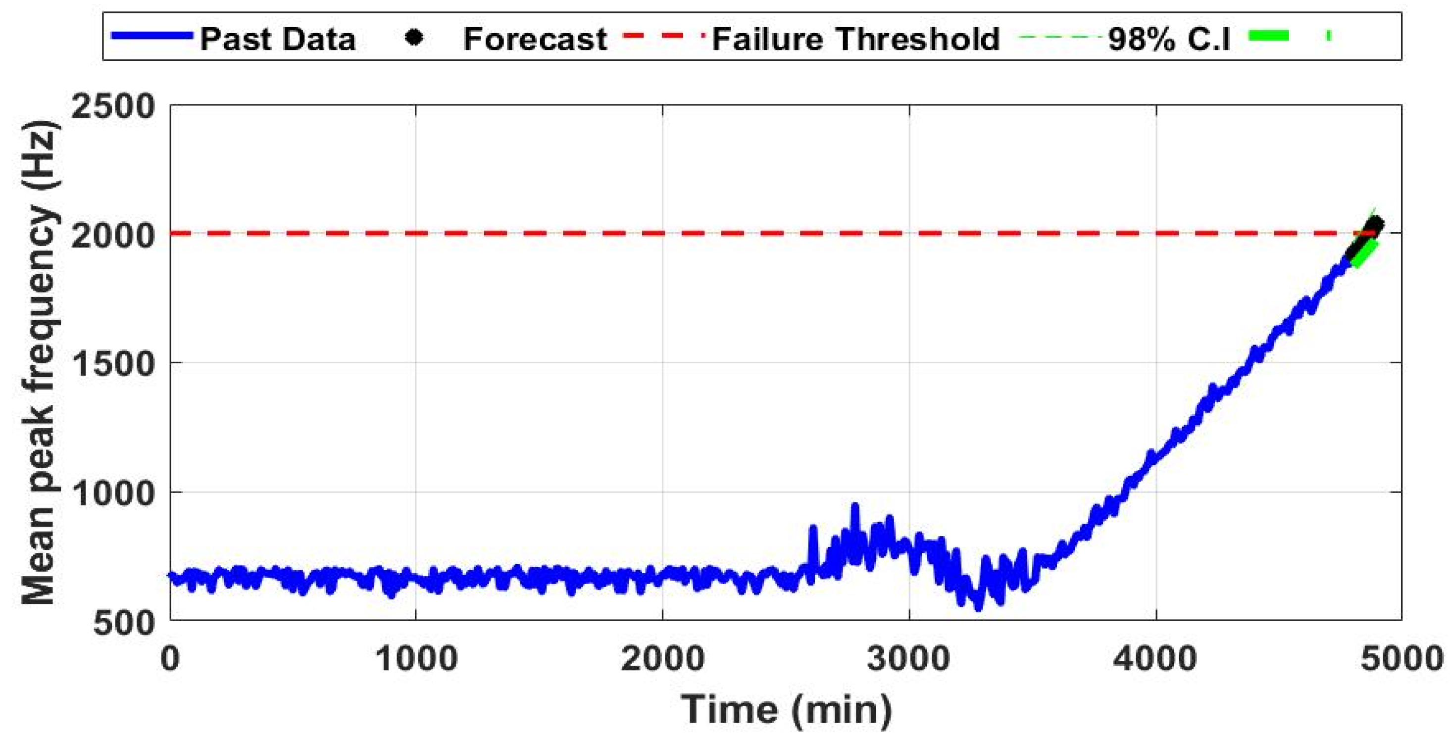
Figure 7 shows the past data, forecast, and failure threshold. It shows that after 4000 min the system will fail, and the accuracy rate is 98% for this analysis.

After data collection, feature extraction was performed by PCA analysis of SVM. Then, the scatter plot was placed to identify different faults in the pumping system. Here, it is seen that the major fault is the cavitation fault. In this research, the authors only concentrated on the cavitation fault for the case study analysis and implemented the ML algorithms (Figure 8).

The hybrid model is used here for fault diagnosis, and LCC analysis of the pump and a vibration signal has been collected as input through an accelerometer; the sampling frequency used here is 25 kHz. Both healthy and three faulty condition vibration signals have been collected. Each failure had several stages, as well as the two states of suddenly closing and opening the valve.

The recognition rate of HMM is shown in

Table 4. The recognition rate of HMM.

Status	Fault Level	Position of Valve	No. of Samples	Correct Recognition	Recognition Rate
Healthy	1	Suddenly closed	250	240	92.14%
	2	Suddenly open	250	310	67.45%
Bearing fault	1	Suddenly closed	250	120	89.45%
	2	Suddenly open	250	69	90.34%
Cavitation	1	Suddenly closed	250	219	96.76%
	2	Suddenly open	250	270	81.90%
Water hammering	1	Suddenly closed	250	340	72.34%
	2	Suddenly open	250	290	88.67%

.

The total no. of samples is 2000, and the average recognition rate is 84.88%.

The table shows that the performance of HMM alone is not good enough.

Now,

Table 5. The recognition rate of SVM.

Status	Fault Level	Position of Valve	No. of Samples	Correct Recognition	Recognition Rate
Healthy	1	Suddenly closed	250	340	98.72%
	2	Suddenly open	250	236	89.34%
Bearing fault	1	Suddenly closed	250	260	88.61%
	2	Suddenly open	250	89	90.12%
Cavitation	1	Suddenly closed	250	178	95.34%
	2	Suddenly open	250	279	94.90%
Water hammering	1	Suddenly closed	250	289	86.34%
	2	Suddenly open	250	210	93.89%

shows the recognition rate of SVM.

The total no. of samples is 2000, and the average recognition rate is 92.15%.

It is seen that the recognition rate for SVM is better than HMM. However, increasing the recognition rate with SVM alone proved exceedingly challenging.

The total no. of samples is 2000, and the average recognition rate is 94.33%.

The hybrid model has improved the average recognition rate (

Table 6. The recognition rate of the hybrid model.

Status	Fault Level	Position of Valve	No. of Samples	Correct Recognition	Recognition Rate
Healthy	1	Suddenly closed	250	480	99.80%
	2	Suddenly open	250	389	97.62%
Bearing fault	1	Suddenly closed	250	367	94.56%
	2	Suddenly open	250	290	91.90%
Cavitation	1	Suddenly closed	250	345	93.25%
	2	Suddenly open	250	460	90.18%
Water hammering	1	Suddenly closed	250	420	89.93%
	2	Suddenly open	250	329	97.42%

).

7. Energy Cost Analysis during Normal and Faulty Conditions

The proposed approach anticipates an equipment breakdown and trains the prediction model. A case study resolves the suggested solution and examines how a pumping system problem affects the LCC cost. The pump was operated in normal conditions to test the LCC cost, and then the cavitation fault was created manually. All the data have been collected both in excellent and harmful conditions. It is seen that if the cavitation problem happens, the flow rate will decrease, and the head value will increase. Thus, the total power and efficiency also will be affected. The efficiency will also drop during the faulty situation.

Despite the higher initial software, microprocessor, and instrumentation costs, the installation cost was slightly more than that of a normal pumping system installation of this size. Common system components including a control valve, an external flow meter, a separate starter, and pipes for the recirculation line are frequently absent, which leads to this problem. The design also reduced costs by removing the need for a bigger pump and motor.

Table 7. Energy cost calculation and other parameters during normal condition.

Flow Rate (m3/h)	Head Value (m)	Total Power (Watt)	Efficiency (%)	Energy Cost per Year (Rs)
3.5	22.18	340	95	421.16
3.3	22.32	360	92	446.31
3.29	22.33	400	91.5	447.005
3.25	22.36	420	90	452.13
3.2	22.4	440	89.5	455.27
3.15	22.42	460	88	462.21
3.1	22.46	480	86	469.57
3	22.53	500	85.5	485.12
2.8	22.65	502	84	519.664
2.56	22.79	510	84.4	568.26
2.5505	22.8	530	83	569.48
2.5504	22.82	535	81	569.57
2.5503	22.83	560	80	570.04
2.5502	22.84	575	79	570.21
2.55	22.85	580	75	570.26

and

Table 8. Energy cost calculation and other parameters during faulty condition.

Flow Rate (m3/h)	Head Value (m)	Total Power (Watt)	Efficiency (%)	Energy Cost per Year (Rs)
2	22.80	105	73	724.96
1.98	22.90	110	72	732.14
1.92	22.98	140	70	743.25
1.9	23.11	180	68	751.59
1.88	23.13	250	65	758.88
1.85	23.16	280	64	797.59
1.7	23.189	300	63	816.05
1.65	23.20	320	62	844.16
1.55	23.24	370	60	924.72
1.38	23.295	380	59	1037.78
1.25	23.33	400	56	1143.14
1.08	23.38	480	55	1358.11
0.8	23.43	500	52	1775.29

show the energy cost per year in different flow rates of the pumping system during normal and faulty conditions. If a fault happens, the flow rate will reduce, the head value will be high, power will decrease, efficiency will decrease, and energy cost will increase. If the overall LCC cost is calculated during normal and faulty conditions, installation, maintenance, and other costs will also be considered.

8. Results and Analysis

Table 9. Life cycle cost in both normal and faulty conditions.

Life Cycle Costs (Rs)	Normal Condition (Rs)	Faulty Condition (Rs)
Initial cost	6,000,000	6,000,000
Installation cost	4,000,000	4,000,000
Energy cost	600,000	900,000
Pump maintenance costs	300,000	800,000
Other maintenance costs	200,000	400,000
Total	11,100,000	12,100,000

shows that faulty condition LCC will be higher, as energy and maintenance costs increase compared to during normal conditions.

In comparison to other machine learning algorithms, like random forest (RF), regression, support vector machine (SVM), K-nearest neighbour (K-NN), and the artificial neural network (ANN) used in the proposed research, SVM and HMM can predict the fault more accurately based on accuracy rate, prediction speed, and training time. Due to their ability to learn from examples, ANN models are frequently used in a variety of academic fields. Furthermore, ANN models outperform conventional machine learning methods when dealing with random, fuzzy, and nonlinear data. Systems with complicated, large-scale structures and ambiguous information best suit ANNs. SVM is a supervised machine learning method that can perform regression analysis, classification, and pattern recognition. SVM has been extensively utilised in industrial equipment predictive maintenance to determine a particular status based on the recorded signal. A network structure called a decision tree has nodes and branches, with nodes made up of intermediate nodes and root nodes. The leaf nodes represent a class level, whereas the intermediate nodes represent a feature.

Random forests are ensembles of regression or classification trees used in nonlinear regression or classification models. Each tree relies on a random vector produced separately from the input. Random forests are ensembles of regression or classification trees used in nonlinear regression or classification models. Each tree relies on a random vector produced separately from the input. The proximity matrices of random forests are another useful feature. A closeness estimate for all sites can be made by looking at whether samples report to the same terminal nodes of all trees. A straightforward and unobtrusive statistical tool for analysing relationships between continuous variables is linear regression. The dependent variable (y-axis) and independent variable (x-axis) are shown in linear regression as having a linear relationship (y-axis). The classifier learner application is now used to analyse and compare each algorithm’s accuracy rate, prediction speed, and training time.

Figure 9 and Figure 10 show the proposed research’s hardware setup and block diagram. Figure 9 shows the multistage parallel pump hardware setup from which all the vibration data, flow rate, and pressure bar data have been collected. Figure 10 shows by flow chart how ML algorithms have been implemented after data collection and feature extraction are carried out. Here, training and testing set have been formed to classify the fault state.

According to

Table 10. Comparison of ML algorithms based on accuracy rate, training time, prediction speed, and energy cost per year.

Algorithms	Accuracy Rate (%)	Training Time (sec)	Prediction Speed (obs/sec)	Energy Cost per Year (Rs)
SVM with HMM	98.7%	0.015	450	1452
K-NN	65%	0.147	220	2989
ANN	81%	1.20	340	3512
Linear regression	72%	1.11	280	4879
Decision tree	56%	1.05	310	5690
Logistic regression	80%	1.00	211	7251
Naïve Bayes	57.30%	1.6	250	4561
Linear discriminant	68%	2	130	5390

and Figure 11, Figure 12, Figure 13 and Figure 14, SVM and HMM perform better than other ML algorithms in terms of accuracy rate, training time, prediction speed, and annual energy cost. Most ML algorithms have been compared by accuracy rate, prediction speed and training time. Based on these three factors, the best-suited algorithm for the particular experiment has been predicted. In the present research, Figure 11 shows that, based on accuracy rate, SVM with HMM is better than other ML algorithms for LCC analysis. Similarly, Figure 12 shows that the training time of SVM and HMM is lesser than different ML algorithms, and Figure 13 shows the prediction speed in the case of SVM and HMM is higher than other ML algorithms. Figure 14 shows if the ML algorithms have been applied for predicting faults in the pumping system in the early stage, and that among all ML algorithms, SVM and HMM predict the fault more efficiently than other algorithms, meaning that energy cost per hour will be lower.

HMM finds the state of the matrix, and this procedure is carried out through probability distribution. The hidden Markov model analyses attempt to recover the sequence of states from observed data. The graph shows the state of the faulty situation. Here, seven nodes are there for faulty conditions. Each node shows the state of the system (Figure 15). HMM is used for the identification of the recognition state of the machine during healthy and faulty situations. Seven nodes are used here for the identification of different states. Among these, only four states are active, as three fault types have been analysed in the present research, and one is a healthy condition.

The graph (Figure 16) shows the transition probability. The probability shows the classes and number of periods and the state of the periods. The graph shows that the system is aperiodic, concluding that the system has been majorly affected.

The graph shows the labels of the state; by these labels, the state condition can be identified (Figure 17).

Here, for SVM and HMM, seven indicators are used. Among these, four are active, as three faulty conditions and one normal condition have been indicated. The transient probability shows each indicator condition (Figure 18).

9. Conclusions

Industrial pumping systems use a lot of energy and money for maintenance and operation. Because engineering and procurement procedures frequently consider only the initial system costs, there are significant opportunities for reducing life cycle system costs that are not taken advantage of. Life cycle cost analysis is a tried and true technique for figuring out the least expensive long-term design or retrofit solutions. The present study shows the importance of LCC cost for the pumping system and its changes due to faulty conditions. It is seen from the analysis that through SVM and HMM hybrid methods based on accuracy, the fault can be predicted early, and energy costs can also be reduced by this method rather than by other ML algorithms. If the energy cost is less, then the life span of the pumping system will be high. In the future, LCC costs will be calculated in a simpler way. The application of AI will be further developed to analyse the LCC of the pumping system and other machinery. Here, SVM is used for the classification of faults and HMM is used for exact fault state identification.

After faults, the pump gives the best operating service between 70 and 75 h; after 82 h, it will stop working.

LCC analysis has been performed during normal and faulty conditions. Then, ML algorithms have been used to identify the faults and reduce the LCC cost of the pump. If SVM and HMM are combined, the overall cost will be reduced.

The suggested research has some restrictions. It does not function well with vast amounts of data, such as DL, and occasionally the performances of the classes are subpar owing to data shortages. The research being used as a case study solely looks at the industrial pump application and does not compare it to other kinds of pump applications. The practical application of the proposed study is the detection of anomalies in industrial multistage pumps requiring constant water supply. The technique can further be evaluated on various machines and different forms of pump fault detection. The authors will give data management greater attention in the near future in order to conduct more studies and enhance performance.

References

1. Zaman, K. Life Cycle Costs (LCC) for wastewater pumping systems. In Proceedings of the Water Environment Federation, New Orleans, LA, USA, 24–28 September 2016. [Google Scholar]
2. Arun Shankar, V.K.; Umashankar, S.; Padmanaban, S.; Paramasivam, S. Adaptive neuro-fuzzy inference system (anfis) based direct torque control of pmsm driven centrifugal pump. IJRER 2017, 7, 1437–1447. [Google Scholar]
3. Tutterow, V.; Hovstadius, G.; McKane, A. Going with the Flow: Life Cycle Costing for Industrial Pumping Systems; Lawrence Berkeley National Lab. (LBNL): Berkeley, CA, USA, 2002. [Google Scholar]
4. Maksimova, S.; Shkileva, A.; Verevkina, E. Life cycle cost and energy conservation for water system pumping station reconstruction. E3S Web Conf. 2020, 164, 01002. [Google Scholar] [CrossRef]
5. Mohanty, A.R.; Pradhan, P.K.; Mahalik, N.P.; Ghosh Dastidar, S. Fault detection in a centrifugal pump using vibration and motor current signature analysis. Int. J. Autom. Control. 2012, 6, 61–76. [Google Scholar] [CrossRef]
6. Fella, G.; Gallipoli, G.; Pan, J. Markov-chain approximations for life-cycle models. Rev. Econ. Dyn. 2019, 34, 183–201. [Google Scholar] [CrossRef] [Green Version]
7. Mohamed, S.E.-D.N.; Mortada, B.; Ali, A.M.; El-Shafai, W.; Khalaf, A.A.M.; Zahran, O.; Dessouky, M.I.; El-Rabaie, E.-S.M.; El-Samie, F.E.A. Modulation format recognition using CNN-based transfer learning models. Opt. Quantum Electron. 2023, 55, 343. [Google Scholar] [CrossRef]
8. Patil, R.B.; Kothavale, B.S.; Waghmode, L.Y.; Pecht, M. Life cycle cost analysis of a computerised numerical control machine tool: A case study from Indian manufacturing industry. J. Qual. Maint. Eng. 2020, 27, 107–128. [Google Scholar] [CrossRef]
9. Chen, Y.; Yuan, J.; Luo, Y.; Zhang, W. Fault Prediction of Centrifugal Pump Based on Improved KNN. Shock. Vib. 2021, 2021, 7306131. [Google Scholar] [CrossRef]
10. Arun Shankar, V.K.; Subramaniam, U.; Padmanaban, S.; Holm-Nielsen, J.B.; Blaabjerg, F.; Paramasivam, S. Experimental Investigation of Power Signatures for Cavitation and Water Hammer in an Industrial Parallel Pumping System. Energies 2019, 12, 1351. [Google Scholar] [CrossRef] [Green Version]
11. Peng, L.; Han, G.; Sui, X.; Pagou, A.L.; Zhu, L.; Shu, J. Predictive approach to perform fault detection in electrical submersible pump systems. ACS Omega 2021, 6, 8104–8111. [Google Scholar] [CrossRef]
12. Don, M.G.; Khan, F. Process fault prognosis using hidden Markov model–bayesian networks hybrid model. Ind. Eng. Chem. Res. 2019, 58, 12041–12053. [Google Scholar]
13. Soualhi, A.; Clerc, G.; Razik, H.; Guillet, F. Hidden Markov models for the prediction of impending faults. IEEE Trans. Ind. Electron. 2016, 63, 3271–3281. [Google Scholar] [CrossRef]
14. Hofmann, P.; Tashman, Z. Hidden markov models and their application for predicting failure events. In Proceedings of the International Conference on Computational Science, Amsterdam, The Netherlands, 3–5 June 2020; Springer: Cham, Switzerland, 2020; pp. 464–477. [Google Scholar]
15. Zhou, Z.J.; Hu, C.H.; Xu, D.L.; Chen, M.Y.; Zhou, D.H. A model for real-time failure prognosis based on hidden Markov model and belief rule base. Eur. J. Oper. Res. 2010, 207, 269–283. [Google Scholar] [CrossRef]
16. Zhao, W.; Shi, T.; Wang, L. Fault diagnosis and prognosis of bearing based on hidden Markov model with multi-features. Appl. Math. Nonlinear Sci. 2020, 5, 71–84. [Google Scholar] [CrossRef]
17. Ocak, H.; Loparo, K.A. A new bearing fault detection and diagnosis scheme based on hidden Markov modeling of vibration signals. In Proceedings of the 2001 IEEE International Conference on Acoustics, Speech, and Signal Processing, Salt Lake City, UT, USA, 7–11 May 2001; Volume 5, pp. 3141–3144. [Google Scholar]
18. Purushotham, V.; Narayanan, S.; Prasad, S.A. Multi-fault diagnosis of rolling bearing elements using wavelet analysis and hidden Markov model based fault recognition. NDT E Int. 2005, 38, 654–664. [Google Scholar] [CrossRef]
19. Jiang, J.; Chen, R.; Chen, M.; Wang, W.; Zhang, C. Dynamic fault prediction of power transformers based on hidden Markov model of dissolved gases analysis. IEEE Trans. Power Deliv. 2019, 34, 1393–1400. [Google Scholar] [CrossRef]
20. Orrù, P.F.; Zoccheddu, A.; Sassu, L.; Mattia, C.; Cozza, R.; Arena, S. Machine learning approach using MLP and SVM algorithms for the fault prediction of a centrifugal pump in the oil and gas industry. Sustainability 2020, 12, 4776. [Google Scholar] [CrossRef]
21. Dutta, N.; Palanisamy, K.; Subramaniam, U.; Padmanaban, S.; Holm-Nielsen, J.B.; Blaabjerg, F.; Almakhles, D.J. Identification of water hammering for centrifugal pump drive systems. Appl. Sci. 2020, 10, 2683. [Google Scholar] [CrossRef] [Green Version]
22. Dutta, N.; Subramaniam, U.; Padmanaban, S. Mathematical models of classification algorithm of Machine learning. QScience Proc. 2019, 1, 3. [Google Scholar]
23. Hashim, Z.S.; Khani, H.I.; Azar, A.T.; Khan, Z.I.; Smait, D.A.; Abdulwahab, A.; Zalzala, A.M. Robust liquid level control of quadruple tank system: A nonlinear model-free approach. Actuators 2023, 12, 119. [Google Scholar] [CrossRef]
24. Nault, J.; Papa, F. Lifecycle assessment of a water distribution system pump. J. Water Resour. Plan. Manag. 2015, 141, A4015004. [Google Scholar] [CrossRef]
25. Dutta, N.; Kaliannan, P.; Paramasivam, S. A comprehensive review on fault detection and analysis in the pumping system. Int. J. Ambient. Energy 2022, 43, 6878–6898. [Google Scholar] [CrossRef]
26. Jayaram, N.; Srinivasan, K. Performance-based optimal design and rehabilitation of water distribution networks using life cycle costing. Water Resour. Res. 2008, 44. [Google Scholar] [CrossRef]
27. Cheng, Q.; Wang, S.; Yan, C. Robust optimal design of chilled water systems in buildings with quantified uncertainty and reliability for minimised life-cycle cost. Energy Build. 2016, 126, 159–169. [Google Scholar] [CrossRef]
28. Kouadri, A.; Hajji, M.; Harkat, M.-F.; Abodayeh, K.; Mansouri, M.; Nounou, H.; Nounou, M. Hidden Markov model based principal component analysis for intelligent fault diagnosis of wind energy converter systems. Renew. Energy 2020, 150, 598–606. [Google Scholar] [CrossRef]
29. Aktaş, A.B. Comparative Life Cycle Cost Analysis of Centrifugal and Positive Displacement Pumps for Mine Dewatering. Master’s Thesis, Middle East Technical University, Ankara, Turkey, 2015. [Google Scholar]
30. Patel, A.; Swathika, O.V.G.; Subramaniam, U.; Babu, T.S.; Tripathi, A.; Nag, S.; Karthick, A.; Muhibbullah, M. A Practical Approach for Predicting Power in a Small-Scale Off-Grid Photovoltaic System using Machine Learning Algorithms. Int. J. Photoenergy 2022, 2022, 9194537. [Google Scholar] [CrossRef]
31. Saon, S.; Hiyama, T. Predicting remaining useful life of rotating machinery based artificial neural network. Comput. Math. Appl. 2010, 60, 1078–1087. [Google Scholar]
32. Salunkhe, T.; Jamadar, N.I.; Kivade, S.B. Prediction of Remaining Useful Life of mechanical components-a Review. Int. J. Eng. Sci. Innov. Technol. 2014, 3, 125–135. [Google Scholar]
33. Rubab, S.; Kandpal, T.C. A financial evaluation of renewable energy technologies for water pumping in rural areas. Int. J. Ambient. Energy 1998, 19, 211–220. [Google Scholar] [CrossRef]
34. Luo, H.; Zhou, P.; Shu, L.; Mou, J.; Zheng, H.; Jiang, C.; Wang, Y. Energy performance curves prediction of centrifugal pumps based on constrained PSO-SVR model. Energies 2022, 15, 3309. [Google Scholar] [CrossRef]
35. Ranawat, N.S.; Kankar, P.K.; Miglani, A. Fault Diagnosis in Centrifugal Pump using Support Vector Machine and Artificial Neural Network. J. Eng. Res. EMSME Spec. Issue 2021, 99, 111. [Google Scholar] [CrossRef]
36. Ranganatha Chakravarthy, H.S.; Bharadwaj, S.C.; Umashankar, S.; Padmanaban, S.; Dutta, N.; Holm-Nielsen, J.B. Electrical fault detection using machine learning algorithm for centrifugal water pumps. In Proceedings of the 2019 IEEE International Conference on Environment and Electrical Engineering and 2019 IEEE Industrial and Commercial Power Systems Europe (EEEIC/I&CPS Europe), Genova, Italy, 11–14 June 2019; pp. 1–6. [Google Scholar]
37. Gao, X.; Pishdad-Bozorgi, P.; Shelden, D.R.; Hu, Y. Machine learning applications in facility life-cycle cost analysis: A review. In Proceedings of the Computing in Civil Engineering 2019: Smart Cities, Sustainability, and Resilience, Atlanta, Georgia, 17–19 June 2019; pp. 267–274. [Google Scholar]
38. Alshathri, S.; Hemdan, E.E.-D.; El-Shafai, W.; Sayed, A. Digital twin-based automated fault diagnosis in industrial IoT applications. Comput. Mater. Contin. 2023, 75, 183–196. [Google Scholar] [CrossRef]
39. Jocanovic, M.; Agarski, B.; Karanovic, V.; Orosnjak, M.; Ilic Micunovic, M.; Ostojic, G.; Stankovski, S. LCA/LCC model for evaluation of pump units in water distribution systems. Symmetry 2019, 11, 1181. [Google Scholar] [CrossRef] [Green Version]
40. Babashamsi, P.; Khahro, S.H.; Omar, H.A.; Rosyidi, S.A.P.; M Al-Sabaeei, A.; Milad, A.; Bilema, M.; Sutanto, M.H.; Yusoff, N.I.M. A Comparative Study of Probabilistic and Deterministic Methods for the Direct and Indirect Costs in Life-Cycle Cost Analysis for Airport Pavements. Sustainability 2022, 14, 3819. [Google Scholar] [CrossRef]
41. Lowe, D.J.; Emsley, M.W.; Harding, A. Predicting construction cost using multiple regression techniques. J. Constr. Eng. Manag. 2006, 132, 750–758. [Google Scholar] [CrossRef] [Green Version]
42. Moon, J.; Park, J.; Hwang, E.; Jun, S. Forecasting power consumption for higher educational institutions based on machine learning. J. Supercomput. 2018, 74, 3778–3800. [Google Scholar] [CrossRef]
43. Zhang, C.; Cao, L.; Romagnoli, A. On the feature engineering of building energy data mining. Sustain. Cities Soc. 2018, 39, 508–518. [Google Scholar] [CrossRef]
44. Bouktif, S.; Fiaz, A.; Ouni, A.; Serhani, M.A. Optimal deep learning lstm model for electric load forecasting using feature selection and genetic algorithm: Comparison with machine learning approaches. Energies 2018, 11, 1636. [Google Scholar] [CrossRef] [Green Version]
45. Ahmed, S.; Azar, A.T.; Tounsi, M. Design of adaptive fractional-order fixed-time sliding mode control for robotic manipulators. Entropy 2022, 24, 1838. [Google Scholar] [CrossRef] [PubMed]
Figure 1. Various parts of the life cycle cost for industrial pump.
Processes 11 02157 g001
Figure 2. The steps for ML algorithm application.
Processes 11 02157 g002
Figure 3. Combination of the SVM and HMM models.
Processes 11 02157 g003
Figure 4. The flow chart of the SVM and HMM application.
Processes 11 02157 g004
Figure 5. The recognition rate of the hybrid model.
Processes 11 02157 g005
Figure 6. Remaining helpful life.
Processes 11 02157 g006
Figure 7. Past, forecast, and failure threshold data.
Processes 11 02157 g007
Figure 8. Various fault analysis through scatter plots in the pumping system.
Processes 11 02157 g008
Figure 9. Hardware setup.
Processes 11 02157 g009
Figure 10. Flow chart of the proposed research.
Processes 11 02157 g010
Figure 11. The accuracy rate of the ML algorithms.
Processes 11 02157 g011
Figure 12. Training time of ML algorithms.
Processes 11 02157 g012
Figure 13. Prediction speed of ML algorithms.
Processes 11 02157 g013
Figure 14. Energy cost per year of various ML algorithms implemented for fault detection.
Processes 11 02157 g014
Figure 15. State of the faulty situation directed by graph.
Processes 11 02157 g015
Figure 16. Transition probability state.
Processes 11 02157 g016
Figure 17. State labels of the HMM.
Processes 11 02157 g017
Figure 18. Indicator transition condition.
Processes 11 02157 g018