Detecting Plant-Wide Oscillation Propagation Effects of Disturbances and Faults in a Chemical Process Plant Using Network Topology of Variance Decompositions

Abstract

This work demonstrates for the first time the application of network topology of variance decompositions in analyzing the connectedness of chemical plant process variable oscillations arising from disturbances and faults. Specifically, the time-based connectedness and frequency-based connectedness of variables can be used to compute the net pairwise dynamic connectedness (NPDC), which originated as a volatility spillover index for financial markets studies in the field of econometrics. This work used the anomaly-detection benchmark Tennessee-Eastman chemical process (TEP) dataset, which consists of 41 measured variables and 11 manipulated variables subjected to various faulty operating conditions. The data analytics was performed using key functions from the R-package ‘ConnectednessApproach’ that implements connectedness computations based on time and frequency. The NPDC coefficient matrices were then transformed into network adjacency matrices for the rendering of the network topology of connectedness for TEP. The resulting network topologies allow a comprehensive analysis of oscillation effects across all plant-measured and manipulated variables. Analyzing the directed connectedness of the system dynamics at short-range, mid-range, and long-range frequencies showed how the oscillation effects of disturbances and faults propagate and dissipate in the short-term, mid-term, and long-term periods.

1. Introduction

1.1. Problem Setup

The complex and nonlinear behavior of many continuous chemical processing systems poses a challenge to the stable operation and the success of control systems to maintain smooth processes within the desired operating conditions. Specifically, the potential system-wide effects of process changes and faults must be quantified to aid in the minimization or elimination of adverse shocks resulting from plant shut-down and re-starts [1,2]. Several works have been completed on the use of various computational techniques to establish protocols and algorithms for detecting anomalies in chemical processing systems exhibiting highly nonlinear dynamics [3]. A common benchmark system used in such efforts is the Tennessee-Eastman chemical process (TEP) dataset originally established by Downs and Vogel [4] and schematically shown in Figure 1. There are five major chemical processing units in the TEP: reactor, product condenser, vapor–liquid separator, recycle compressor, and product stripper (Figure 1). The TEP involves the production of two liquid product components, G and H, from four gaseous reactants, A, C, D, and E, with an additional inert B and a byproduct F as shown in the following four reaction steps [4].

$$A_{\left(g\right)}+C_{\left(g\right)}+D_{\left(g\right)}\to G_{\left(liq\right)}$$

(R1)

$$A_{\left(g\right)}+C_{\left(g\right)}+E_{\left(g\right)}\to H_{\left(liq\right)}$$

(R2)

$$A_{\left(g\right)}+E_{\left(g\right)}\to F_{\left(liq\right)}$$

(R3)

$$3D_{\left(g\right)}\to F_{\left(liq\right)}$$

(R4)

1.2. Challenge of Oscillation Propagation and Root-Cause Analysis

Oscillation propagation and root-cause analysis have always been active study topics in chemical processing because of their importance in minimizing variations in process outputs such as product stream at a certain purity, flow rate, etc. [5]. The interconnection of process units makes this analysis task even more challenging [1]. Previous works have demonstrated the adaptability of algorithms and computations in econometrics for use in chemical process oscillation analysis [1,6]. Such adaptations of econometrics techniques for chemical process dynamics analysis naturally occur due to the inherent similarities in the feedback loop mechanisms designed to achieve stability in both fields, as depicted in Figure 2. One commonly used econometrics technique applied in various fields is the Granger causality [5], which is a hypothesis testing-based approach to estimating cause–effect relations of multivariate systems that originated from the study of financial markets [7]. Though Granger causality is effective in many econometrics analyses on causality, many studies have illustrated the limitations of the technique in applications outside econometrics, with one main issue being the impact of the vector autoregressive (VAR) model properties on the conditional causality estimates [8,9]. This issue is solved by a recently established econometric technique originated by Diebold and Yılmaz [10] that uses generalized variance decomposition in which the forecast-error variance decompositions are invariant to the variable ordering [11]. The said technique produces a “connectedness” matrix that can eventually be treated as an adjacency matrix for network topology rendering [12]. The extended form of the technique using frequency-based decomposition of variance can capture periodic trends [13] that are inherent in oscillation propagations [1]. This work demonstrates for the first time the application of network topology of variance decompositions in detecting the effects of oscillations arising from disturbances and faults in a chemical process.

1.3. Objectives of the Work

This work aims to show how key concepts and techniques on the analysis of volatility spillover in financial systems developed in the field of econometrics can be adopted as analysis tools in improving the understanding of the dynamic behavior of chemical processing systems. The study dataset is the TEP benchmark dataset [4,16], with sample renderings in Figure 3 and Figure A3. The specific objectives of the paper are:

• To explain how the dynamics of a chemical process such as the TEP can be modeled to compute measures of multivariate connectedness,
• To show how the measures of variable connectedness are represented as network graphs for visual analysis of system volatility,
• To perform the computations and network rendering of connectedness using two connectedness dimensions: time connectedness and frequency connectedness
• To discuss how the findings on the use of network topology of variance decompositions for volatility spillover analysis in a chemical process may complement and perhaps advance chemical process design and control.

2. Methodology

2.1. Theory: A Solution—Multivariate Time-Series Variance Decompositions and Their Connectedness

The analysis of volatility spillover effects and variable connectedness is integral to the study of financial systems and the practice of risk measurement and management; hence, the field of econometrics has developed and advanced numerous data analytics techniques and algorithms on the subject [17]. One recently developed technique that provides numerical and visual metrics for estimating spillover effects is the technique of network topology of variance decompositions. To put the solution approach into the framework of chemical process dynamics and control, the two concepts (1) variance decompositions and (2) network topology will now be presented in brief, along with citations of relevant pioneering papers that provide more details on the theories and computational mechanics of such concepts and techniques [10,12,13].

2.1.1. Variance Decomposition—Estimating Multivariate Connectedness

Consider a $N$-variate dynamical system evolving in time with $N$ dynamical variables $x=\left[x_1,\dots x_N\right]\prime$. Denote a vector time series of the $x$ variables as $x_{∎,t}$ taken at time $t=1,\dots ,T$ (Equation (1)), which is the vector representation of the TEP dynamics graphically shown in Figure 3:

$$x_{∎,t}=\left[x_{1,t},\dots x_{N,t}\right]\prime$$

(1)

The variance decomposition starts by de-noising the data. This is conducted by using a time-series model that can capture trends, and a common effective model is the vector autoregressive (VAR) model of order $p$ [10,12]. Therefore,

$$x_{∎,t}={\mathsf{\Phi }}_1{x}_{t-1}+\dots +{\mathsf{\Phi }}_p{x}_{t-p}+{ϵ}_t$$

(2)

where ${\mathsf{\Phi }}_1\dots {\mathsf{\Phi }}_p$ are the coefficients of the regressed VAR model in which the regression is calculated such that each variable is regressed on its own $p$ lags and the $p$ lags of each of the other variables. The ${ϵ}_t$ is white noise with covariance matrix $\Sigma$. For simplicity of succeeding derivations, the VAR model can be concisely written as an $N\times N$ matrix of lag-polynomials $L$ and the identity matrix $I_N$ [10]:

$$\Phi \left(L\right)=\left[I_N-{\mathsf{\Phi }}_{1}L-\dots -{\mathsf{\Phi }}_p{L}^p\right]$$

(3)

This $\Phi \left(L\right)$ represents the optimized VAR model capturing the trends in the data such that the residuals are the white noise ${ϵ}_t$. Therefore, the VAR model can be written concisely as [13]:

$$\Phi \left(L\right)x_t={ϵ}_t$$

(4)

The VAR coefficients ${\mathsf{\Phi }}_1\dots {\mathsf{\Phi }}_p$ in matrix $\Phi \left(L\right)$ that represent de-noised time-series trends can be used to compute the moving average (MA) matrix coefficients $\Psi \left(L\right)$, i.e., $\Phi \left(L\right)={\left[\Psi \left(L\right)\right]}^{-1}$, such MA is a good approximation of $x_{∎,t}$ at varying MA horizons $h=1,\dots ,H$, with coefficients ${\Psi }_h$ [13]:

$$x_{∎,t}\approx {\Psi }_h{ϵ}_t$$

(5)

The MA coefficients ${\Psi }_h$ can then be transformed to calculate the matrix of generalized variance decompositions using the following formula according to Diebold and Yılmaz [10,13], where ${\sigma }_{kk}={\Sigma }_{k,k}$:

$${\left({\theta }_H\right)}_{j,k}=\frac{{\sigma }_{kk}^{-1}{\sum }_{h=0}^H{\left({\left({\Psi }_h\Sigma \right)}_{j,k}\right)}^2}{{\sum }_{h=0}^H{\left({\Psi }_h\Sigma {\Psi }_h^{\prime }\right)}_{j,j}}$$

(6)

The matrix coefficient ${\left({\theta }_H\right)}_{j,k}$ is the “connectedness” measure and denotes the contribution of the $k$-th variable to the variance of forecast error of the $j$-th variable at horizon h [10]. To finalize the connectedness metric $C_H$, the coefficients in matrix ${\theta }_H$ must be normalized by the row sum [13] as shown in Equation (7), and the connectedness metrics must be defined as the forecast contributed by errors other than own errors [10] as shown in Equation (8):

$${\left({\tilde{\theta }}_H\right)}_{j,k}=\frac{{\left({\theta }_H\right)}_{j,k}}{{\sum }_{k=1}^N{\left({\theta }_H\right)}_{j,k}}$$

(7)

$$C_H=100{\displaystyle \bullet }\frac{{\sum }_{j\ne k}{\left({\tilde{\theta }}_H\right)}_{j,k}}{\sum {\left({\tilde{\theta }}_H\right)}_{j,k}}$$

(8)

The matrix $C_H$ consists of the variance decompositions of the $N$-variate dynamical system with variable measurements $x_{∎,t}$.

Table 1. Connectedness table schematic for $C_H$ of the variables $x=\left[x_1,\dots x_N\right]\prime$.

	${\mathit{x}}_1$	${\mathit{x}}_2$	$\dots$	${\mathit{x}}_{\mathit{N}}$
$x_1$	$c_{11}^H$	$c_{12}^H$	$\dots$	$c_{1N}^H$
$x_2$	$c_{21}^H$	$c_{22}^H$	$\dots$	$c_{2N}^H$
$⋮$	$⋮$	$⋮$	$\ddots$	$⋮$
$x_N$	$c_{N1}^H$	$c_{N2}^H$	$\dots$	$c_{NN}^H$

below symbolically shows the elements of the matrix $C_H$, where each $c_{jk}^H$ is a connectedness coefficient from variable $x_j$ to variable $x_k$. Transforming the data shown in the matrix $C_H$ to a network graph is presented in the next section.

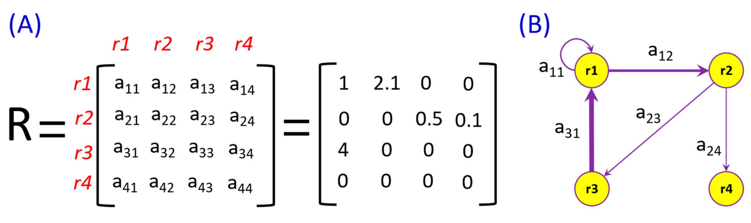
2.1.2. Network Topology—Graphs of Connectedness

The network graph of the variable connectedness measures in a multivariate system such as TEP is a valuable tool in analyzing the influences of variables and volatility spillover effects in the system. After computing the connectedness coefficients matrix $C_H$ (Table 1), the network representation of the coefficients can now be carried out by treating the $C_H$ matrix as an adjacency matrix [12]. Among the various centrality measures in a network, the directed centralities of in-degree, out-degree, and net directed degree are the most relevant in the task of estimating volatility spillover [10]. Below is an illustration of how an adjacency matrix is rendered as a network graph.

For simplicity, consider as a toy example the small adjacency matrix $R$ of four variables $r={\left[r_1,r_2,r_3,r_4\right]}^{\prime }$, as shown in Figure 4.

In the network graph (Figure 4), the variables $r_1,r_2,r_3$, and $r_4$ become nodes, and the connection between two nodes is an edge. The coefficient on the $R$ matrix (Figure 4A) is the weight of an edge connecting two nodes in the “row-to-column” direction. Hence, a weight of zero (0) means no connection between variables in a particular direction. In order to model the direction of influence, the network must be transformed into a directed graph, as shown above. Note that there is a self-directed edge “$r_1$ to $r_1$” in the graph for network $R$ (Figure 4B), but this kind of self-connectedness is excluded in the $C_H$ matrix as the definition of connectedness to “itself” does not add relevant information [10].

2.2. Computations: On TEP Benchmark Dataset Using the R-Package “ConnectednessApproach”

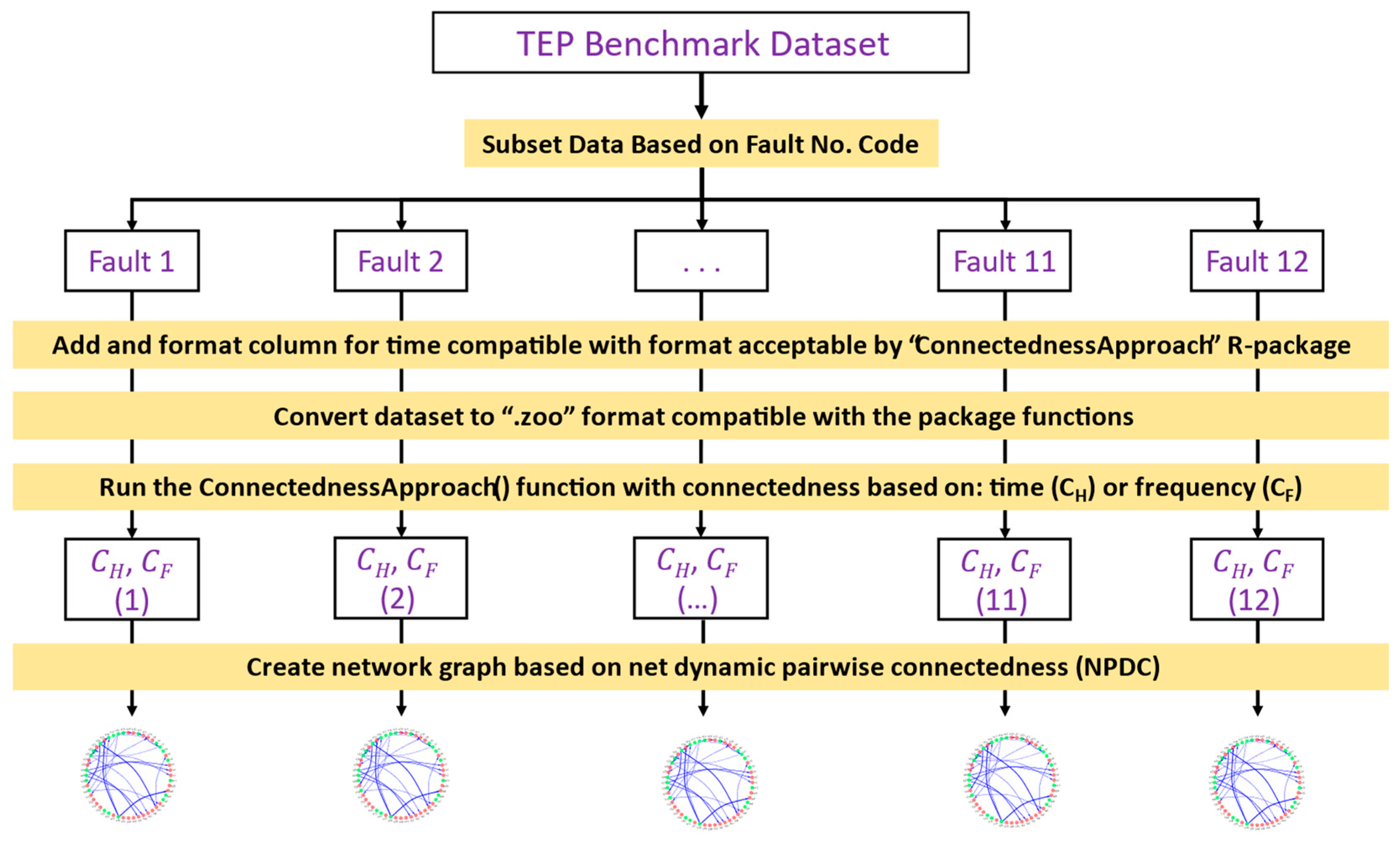
2.2.1. Data Analytics Workflow

A schematic of the data analytics workflow is shown in Figure 5. The steps were implemented via the R-codes [18] and R-Studio [19] written for the work and provided through an online GitHub repository Fortela and Mikolajczyk [20] (https://github.com/dhanfort/TEP_connectedness.git (accessed on 16 April 2023)). The R codes were built around the main analysis R-package “ConnectednessApproach” (version 1.0.1) created by Gabauer [21] and implemented the computations discussed in the theory section (see Section 2.1 of this paper).

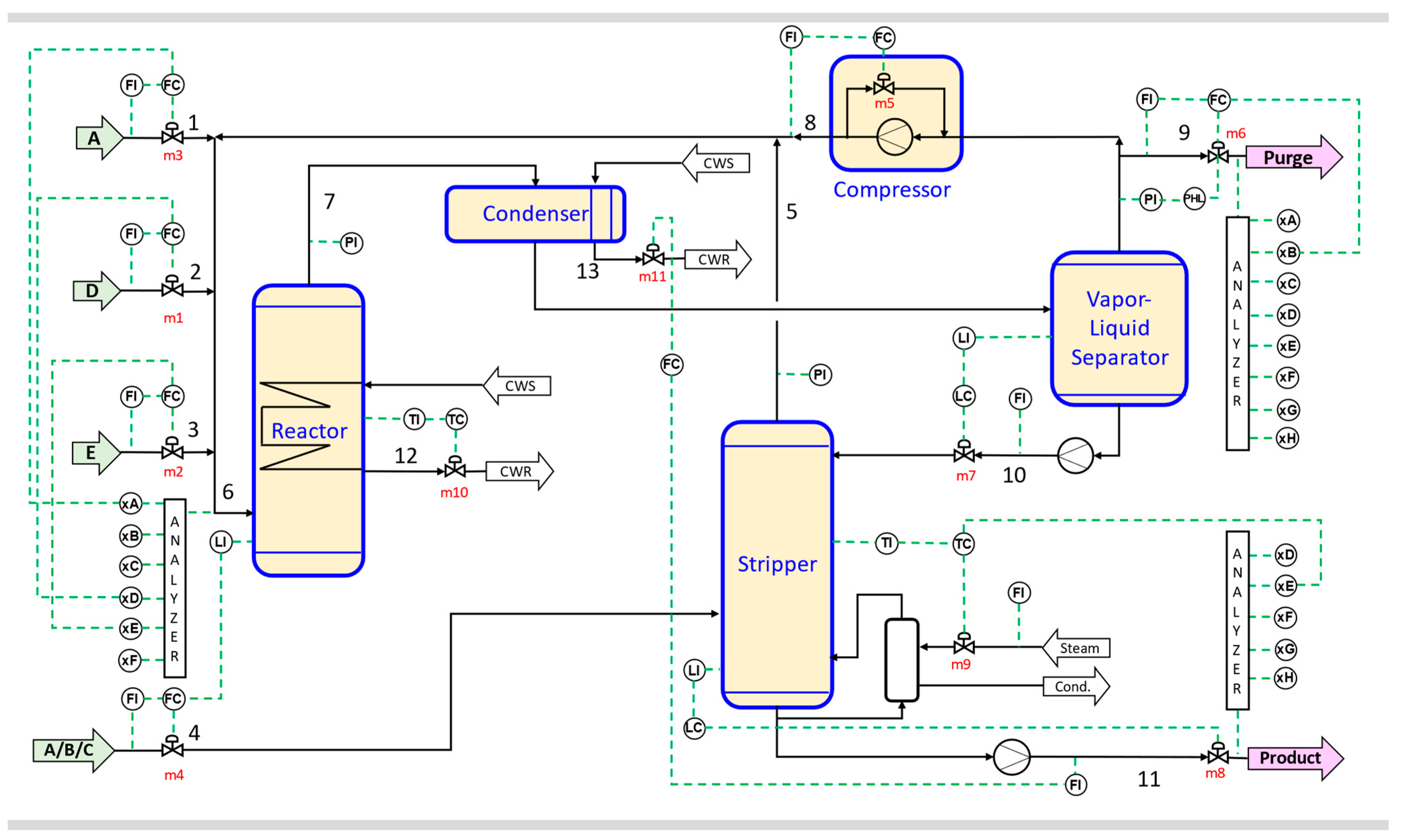
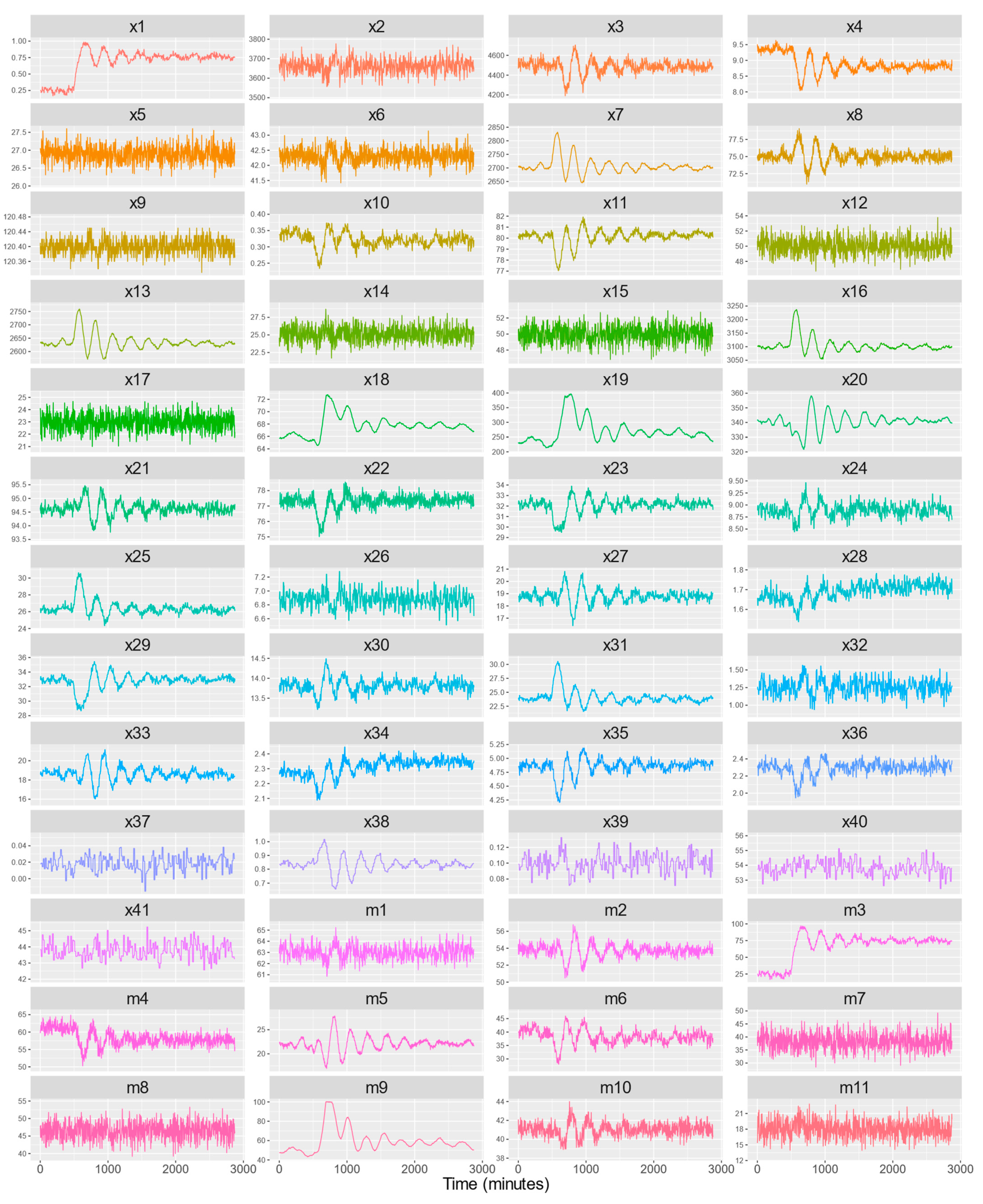
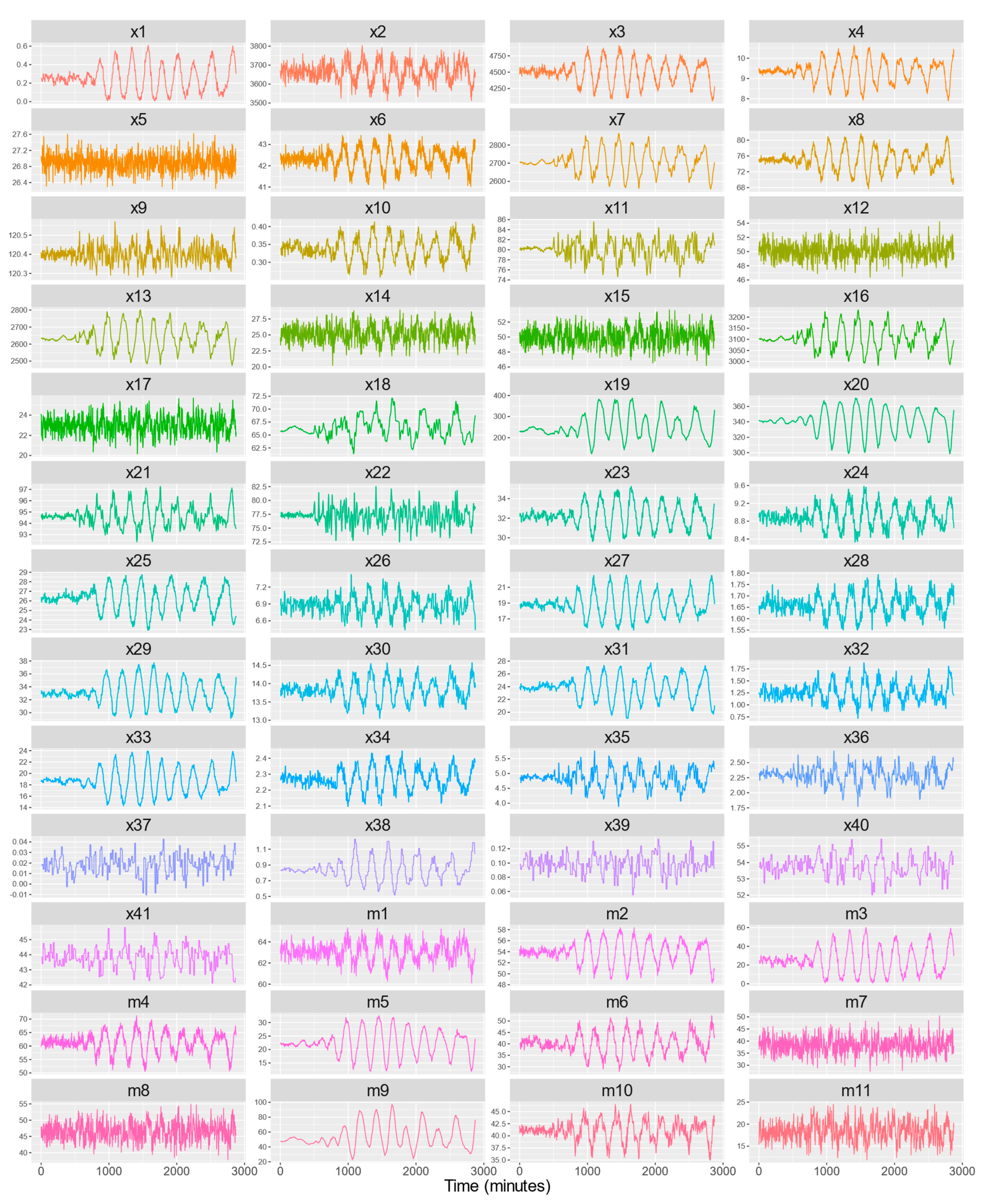
2.2.2. Benchmark Dataset: Tennessee-Eastman Chemical Process (TEP)

The dataset used in this work is that of the TEP process, which has been used as a benchmark process [4,16]. The particular TEP dataset used in this work is the recently expanded version created by Rieth et al. [3,16] with the aim of providing more variations of TEP for anomaly detection applications. There are 41 measured variables (coded as x1 to x41) and 11 manipulated variables (coded as m1 to m11), which are defined in

Table 2. Definition of process variables and symbols in the TEP benchmark dataset based on Downs and Vogel [4].

Current Symbol	Variable Definition	Original Symbol [4]	Units
x1	A feed (stream 1)	XMEAS (1)	kscmh
x2	D feed (stream 2)	XMEAS (2)	kg/h
x3	E feed (stream 3)	XMEAS (3)	kg/h
x4	A and C feed (stream 4)	XMEAS (4)	kscmh
x5	Recycle flow (stream 8)	XMEAS (5)	kscmh
x6	Reactor feed rate (stream 6)	XMEAS (6)	kscmh
x7	Reactor pressure	XMEAS (7)	kPa gauge
x8	Reactor level	XMEAS (8)	%
x9	Reactor temperature	XMEAS (9)	°C
x10	Purge rate (stream 9)	XMEAS (10)	kscmh
x11	Product separator temperature	XMEAS (11)	°C
x12	Product separator level	XMEAS (12)	%
x13	Product separator pressure	XMEAS (13)	kPa gauge
x14	Product separator underflow (stream 10)	XMEAS (14)	m3/h
x15	Stripper level	XMEAS (15)	%
x16	Stripper pressure	XMEAS (16)	kPa gauge
x17	Stripper underflow (stream 11)	XMEAS (17)	m3/h
x18	Stripper temperature	XMEAS (18)	°C
x19	Stripper steam flow	XMEAS (19)	kg/h
x20	Compressor work	XMEAS (20)	kW
x21	Reactor cooling water outlet temperature	XMEAS (21)	°C
x22	Separator cooling water outlet temperature	XMEAS (22)	°C
x23	A mole % reactor feed (stream 6)	XMEAS (23)	mol%
x24	B mole % reactor feed (stream 6)	XMEAS (24)	mol%
x25	C mole % reactor feed (stream 6)	XMEAS (25)	mol%
x26	D mole % reactor feed (stream 6)	XMEAS (26)	mol%
x27	E mole % reactor feed (stream 6)	XMEAS (27)	mol%
x28	F mole % reactor feed (stream 6)	XMEAS (28)	mol%
x29	A mole % purge gas (stream 9)	XMEAS (29)	mol%
x30	B mole % purge gas (stream 9)	XMEAS (30)	mol%
x31	C mole % purge gas (stream 9)	XMEAS (31)	mol%
x32	D mole % purge gas (stream 9)	XMEAS (32)	mol%
x33	E mole % purge gas (stream 9)	XMEAS (33)	mol%
x34	F mole % purge gas (stream 9)	XMEAS (34)	mol%
x45	G mole % purge gas (stream 9)	XMEAS (35)	mol%
x36	H mole % purge gas (stream 9)	XMEAS (36)	mol%
x37	D mole % product (stream 11)	XMEAS (37)	mol%
x38	E mole % product (stream 11)	XMEAS (38)	mol%
x39	F mole % product (stream 11)	XMEAS (39)	mol%
x40	G mole % product (stream 11)	XMEAS (40)	mol%
x41	H mole % product (stream 11)	XMEAS (41)	mol%
m1	D feed flow valve opening (stream 2)	XMV (1)	% open
m2	E feed flow valve opening (stream 3)	XMV (2)	% open
m3	A feed flow valve opening (stream 1)	XMV (3)	% open
m4	A and C feed flow valve opening (stream 4)	XMV (4)	% open
m5	Compressor recycle valve opening	XMV (5)	% open
m6	Purge valve opening (stream 9)	XMV (6)	% open
m7	Separator pot liquid flow valve opening (stream 10)	XMV (7)	% open
m8	Stripper liquid product flow valve opening (stream 11)	XMV (8)	% open
m9	Stripper steam valve opening	XMV (9)	% open
m10	Reactor cooling water flow valve opening	XMV (10)	% open
m11	Condenser cooling water flow valve opening	XMV (11)	% open

Note that the vector of process variables consists of both of the variables x1, x2, …, x41 and of the variables m1, m2, …, m11, as summarized in Table 2.

based on the original definitions and data of Downs and Vogel [4]. Note that the vector of process variables consists of both of the variables x1, x2, …, x41 and of the variables m1, m2…, m11, as summarized in Table 2. That is, $x={\left[x_1,x_2,\dots ,x_{41},m_1,m_2,\dots ,m_{11}\right]}^{\prime }$. More details about the TEP dataset and how to download it are available on the dataset webpage by Rieth et al. [16]. A sample rendering of the TEP dynamics in a normal operation is shown in Figure 3 for the data subset with “Fault 1” setting. As shown in Figure 1, the TEP benchmark process includes feedback controllers with valve openings as the manipulated variable at various key locations to control specific process variables.

The various TEP process faults are summarized in

Table 3. Faults and distrubances in the TEP benchmark dataset based on Downs and Vogel [4].

Fault No.	Fault Description	Type
1	A/C feed ratio, B composition constant (stream 4)	Step Change
2	B composition, A/C ratio constant (stream 4)	Step Change
3	D feed temperature (stream 2)	Step Change
4	Reactor cooling water inlet temperature	Step Change
5	Condenser cooling water inlet temperature	Step Change
6	A feed loss (stream 1)	Step Change
7	C heater pressure loss—reduced availability (stream 4)	Step Change
8	A, B, C feed composition (stream 4)	Random Variation
9	D feed temperature (stream 2)	Random Variation
10	C feed temperature (stream 4)	Random Variation
11	Reactor cooling water inlet temperature	Random Variation
12	Condenser cooling water inlet temperature	Random Variation

. Note that there are 20 sub-routines to create settings of faults; hence, there are 20 faults in the TEP benchmark dataset (Fault 1 to Fault 20) originally run via Fortran by Downs and Vogel [4], but only Fault 1 to Fault 15 have known process dynamics fault settings in the sub-routine code. The remaining sub-routines can be programmed by the user [4], but this current work did not need to run the other fault subroutines because the original dataset fault settings Fault 1 to Fault 12 were determined to be enough for the analysis in this current work.

Overall, the TEP dataset used consists of 52 process variables (x1…x41 plus m1…m11), 960 time steps with a time step interval of 3 min (total process dynamics period of 2880 min), and 12 fault settings. Figure 3 is a sample rendering for the “Fault 1” setting. Hence, $x={\left[x_1,x_2,\dots ,x_{41},m_1,m_2,\dots ,m_{11}\right]}^{\prime }$, $N$ = 52, and $T$ = 960. The resulting connectedness matrix for each fault setting has a dimension $N\times N$, which is $52\times 52$.

2.2.3. Type of Connectedness

• Time Connectedness

The current econometrics literature on the subject of variance decomposition shows various ways of modeling the connectedness metric. Connectedness in time is estimated by the $C_H$ matrix derived in Section 2.1 theory section. This is because the forecasting step at varying time horizons $h=1,\dots ,H$ computes the effect of one variable to another at $h$ steps ahead in time [10,17]. In the R-package “ConnectednessApproach”, the core function that implements this computation in the time domain is the “TimeConnectedness()” that is accessed by other functions such as the “ConnectednessApproach()” function.

2.

Frequency Connectedness

Building on the work of Diebold and Yılmaz [10], Baruník and Křehlík [13] expanded the variance decomposition to use Fourier transforms in decomposing time-series dynamics according to frequencies. In the R-package, frequency connectedness is implemented by the core function “FrequencyConnectedness()” that is accessed by other functions, such as the “ConnectednessApproach()” function.

For the “frequency connectedness” $C_F$, connectedness in short-term, mid-term, and long-term periods can be modeled by specifying the partitioning of the domain of the Fourier transforms defined in the interval $\left[-\pi ,\pi \right]$ based on Baruník and Křehlík [13]. More partitions mean higher frequencies, equivalently modeling short-term effects; on the other hand, fewer partitions (including no partition) mean low frequencies, equivalently modeling long-term effects [13]. This work used the following three levels of partitions to model short-term, mid-term, and long-term effects, respectively: $\left[\pi ,\raisebox{1ex}{$\pi $}\!\left/ \!\raisebox{-1ex}{$2$}\right.,0\right]$, which are the default partition levels in the R-package function for frequency connectedness analysis [13,21]. When converted to the common way of reporting frequencies, considering that the TEP dataset is for a process dynamics duration of 2880 min, these partitions correspond to the partition intervals of [917.2 min, 1834.4 min, and 2880 min], respectively; hence resulting to the following sampling frequencies: [1/55,032 Hz, 1/110,063 Hz, and 1/172,800 Hz] for short-, mid-, and long-term effects.

2.2.4. Process Variables Connectedness Reporting Using Volatility Spillover Index

Aggregating the values of the connectedness matrix $C_H$ or $C_F$ can be conducted in various ways for econometrics applications, but the index that measures how shocks are transmitted across financial markets is the net pairwise dynamic connectedness (NPDC) that is computed from the connectedness matrix [22]. Hence, this work uses NPDC as a measure of the volatility index in a chemical process such as TEP. The computation of NPDC can be conveniently specified in the “ConnectednessApproach()” function [21]. Depending on the tolerance of risk, only a certain range of NPDC values are considered for network topology rendering. It is typical for financial analysis to use a threshold of 25% (or threshold of 0.25) of the bivariate NPDC as the minimum level of NPDC used for spillover analysis [21]. This work evaluates how this threshold on volatility index NPDC affects the network topology of TEP.

The network graph renderings were completed using the “igraph” R-package [23] with the circle layout in such a way that the node positions are fixed, allowing easy trends tracking of network connectedness. The weight of the NPDC between variables is graphically represented as the thickness of the directed edges. That is, a thick, directed edge means a large bivariate NPDC index. Arrows on the edges represent the direction of the volatility spillover effect [21].

3. Results and Discussion

First, the vector autoregressive (VAR) model residuals from the dataset are evaluated using hypothesis testing against the null hypothesis that the mean of the residuals is not different from zero (

Table 4. Hypothesis testing on the standardized residuals as a measure of white noise ${ϵ}_t$ from the VAR model of each TEP fault dataset using a two-sided t-test.

Fault No.	Mean of Standardized Residuals	Degrees of Freedom	t-Statistic	p-Value Two-Sided t-test	$\mathbf{Decision} \mathbf{at} \mathbf{Significance} \mathbf{Level} \mathit{\alpha }$
					$\mathit{\alpha }=0.05$	$\mathit{\alpha }=0.01$
1	28.66	2703	1.8129	0.06995	$\mathrm{Fail} \mathrm{to} \mathrm{Reject} H_0$	$\mathrm{Fail} \mathrm{to} \mathrm{Reject} H_0$
2	30.92	2703	1.9395	0.05254	$\mathrm{Fail} \mathrm{to} \mathrm{Reject} H_0$	$\mathrm{Fail} \mathrm{to} \mathrm{Reject} H_0$
3	30.84	2703	1.9615	0.05000	$\mathrm{Reject} H_0$	$\mathrm{Fail} \mathrm{to} \mathrm{Reject} H_0$
4	28.45	2703	1.8305	0.06728	$\mathrm{Fail} \mathrm{to} \mathrm{Reject} H_0$	$\mathrm{Fail} \mathrm{to} \mathrm{Reject} H_0$
5	28.59	2703	1.7647	0.07773	$\mathrm{Fail} \mathrm{to} \mathrm{Reject} H_0$	$\mathrm{Fail} \mathrm{to} \mathrm{Reject} H_0$
6	10.20	2703	1.8913	0.05870	$\mathrm{Fail} \mathrm{to} \mathrm{Reject} H_0$	$\mathrm{Fail} \mathrm{to} \mathrm{Reject} H_0$
7	31.66	2703	1.9764	0.04821	$\mathrm{Reject} H_0$	$\mathrm{Fail} \mathrm{to} \mathrm{Reject} H_0$
8	25.75	2703	1.5543	0.12020	$\mathrm{Fail} \mathrm{to} \mathrm{Reject} H_0$	$\mathrm{Fail} \mathrm{to} \mathrm{Reject} H_0$
9	30.76	2703	1.9507	0.05120	$\mathrm{Fail} \mathrm{to} \mathrm{Reject} H_0$	$\mathrm{Fail} \mathrm{to} \mathrm{Reject} H_0$
10	31.19	2703	1.9776	0.04808	$\mathrm{Reject} H_0$	$\mathrm{Fail} \mathrm{to} \mathrm{Reject} H_0$
11	30.86	2703	1.9541	0.05079	$\mathrm{Fail} \mathrm{to} \mathrm{Reject} H_0$	$\mathrm{Fail} \mathrm{to} \mathrm{Reject} H_0$
12	31.48	2703	1.7588	0.07872	$\mathrm{Fail} \mathrm{to} \mathrm{Reject} H_0$	$\mathrm{Fail} \mathrm{to} \mathrm{Reject} H_0$

). This is a fundamental assumption about white noise, ${ϵ}_t$ as detailed in Section 2.2.1, which is left after the VAR model captures the trends in the data. Then, the network topology of oscillation propagation measured by the NPDC index for Fault 1 to Fault 12 is presented for time-based connectedness (Figure 6 and Figure 7). Afterward, the effect of varying the minimum threshold bivariate NPDC index in network topology is evaluated for time-based connectedness on Fault 12, as shown in Figure 8. Finally, the volatility spillover network topology based on frequency connectedness is presented using Figure 9 for Fault 1 and Figure 10 for Fault 12. For reference to the type of data used to create network graphs, a sample NPDC matrix for time-connectedness and frequency-connectedness is shown in Appendix A for TEP setting Fault 12 (Figure A1 and Figure A2).

3.1. VAR Model Residuals Analysis

Hypothesis testing on the white noise ${ϵ}_t$ (Equation (2)) must be conducted to make sure that the VAR model captures the trends in the time-series data. The time-series residuals were embedded into one-dimensional representation according to established computations from previous works on time-series embedding. That is, the time-series residuals of one variable were embedded into one dimension representation. Since one fault dataset has 52 variables, a VAR model embedded residuals of $52\times 52$ matrix was created, resulting in a total of $52\times 52=2704$ one-dimension VAR residuals. Hence, the VAR model residuals for each variable were normalized by the standard deviation of each corresponding variable. This was followed by a two-sided t-test, with degrees-of-freedom = no. samples −1 = 2704 −1 = 2703, on the standardized residuals with the null hypothesis that the mean is equal to zero, i.e., $H_0: {\mu }_{ϵ}=0$, and the alternative hypothesis that the mean is not equal to zero, i.e., $H_A: {\mu }_{ϵ}\ne 0$. The analysis was conducted for all the TEP fault datasets (Fault 1 to Fault 12), as summarized in Table 4. The R-code for this analysis is included in the online GitHub repository for the project [20].

These hypothesis testing results show that the residuals are not different from zero at a significance level of 1% ($\alpha =0.01$) in all fault settings (Fault 1 to Fault 12). If the significance level is increased to 5% ($\alpha =0.05$), then a few datasets, i.e., Fault 3, Fault 7, and Fault 10, result in rejecting the null hypothesis that the residuals are equal to zero for these fault settings (Table 4). The level of significance to be used can vary depending on the strictness of the hypothesis testing because $\alpha$ is a measure of the strength of the evidence that must be present in the dataset before rejecting the null hypothesis. However, with a large degrees-of-freedom of 2703 (with 2704 samples per fault dataset), the use of the VAR model in denoising the TEP datasets and capturing the trends at a significance level $\alpha =0.01$ is warranted.

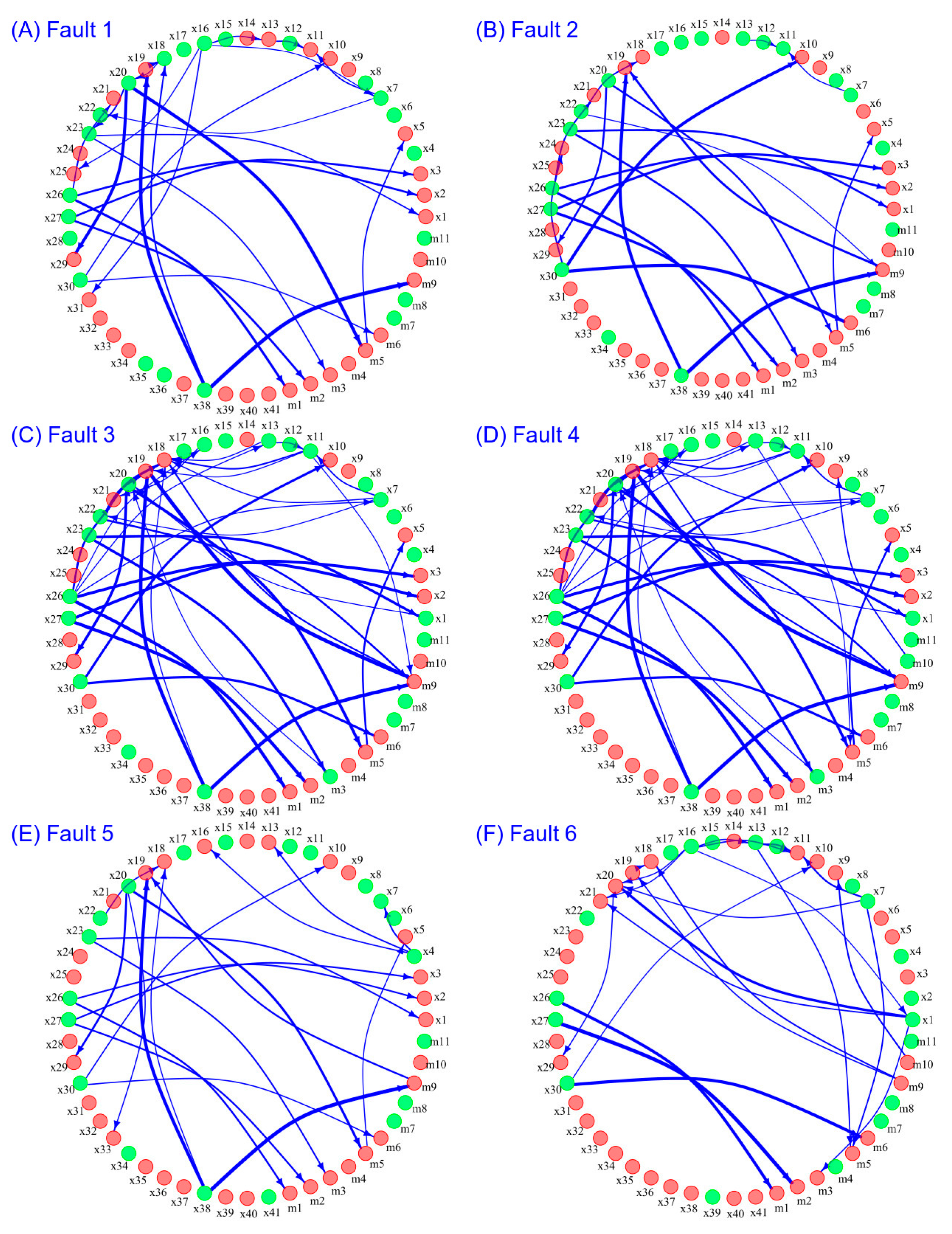
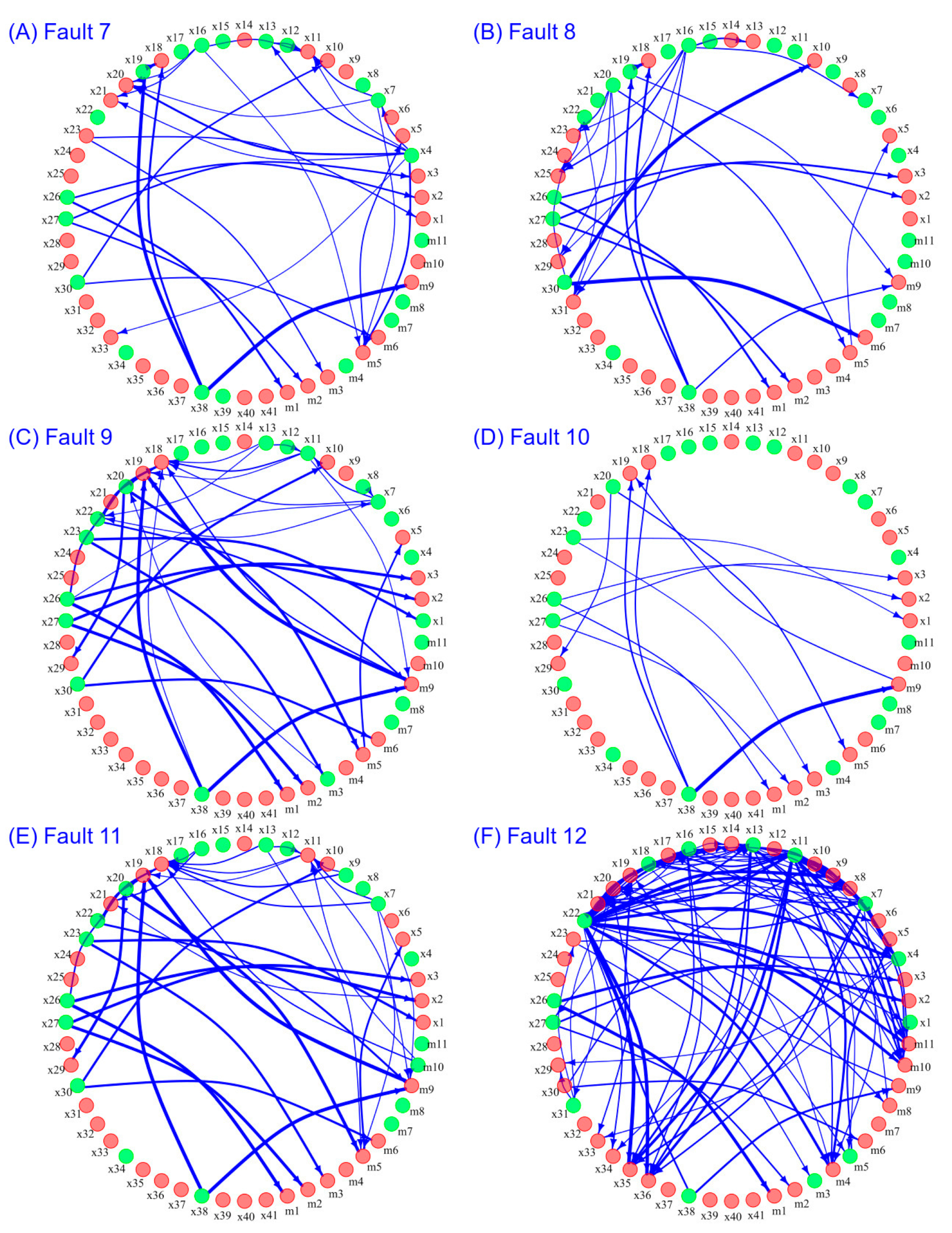
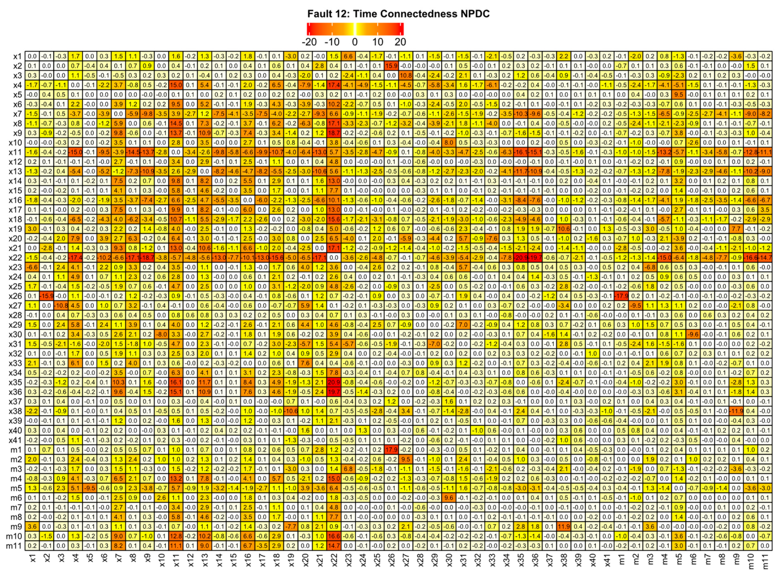
3.2. Oscillation Propagation Effects from TEP Faults Based on Time Connectedness

Depending on the dynamics of the fault, the network topology based on the NPDC index varies from Fault 1 to Fault 12 (Figure 6 and Figure 7). The fault that has the most volatility connectedness is Fault 12 (Figure 7F), when the condenser cooling water inlet temperature randomly fluctuated (Table 3). The fault that has the least volatility, as indicated by few node connections and thin directed edges, is Fault 10 (Figure 7D), when the reactor cooling water inlet temperature randomly fluctuated.

The main task of this work is to discuss how consistent the trends of NPDC networks are with the mechanistic relations of the variables in the TEP process to be able to assess the potential of the network topology of variance decompositions in capturing the volatility effects in the TEP. This will now be addressed by focusing on the key trends of network topologies (Figure 6 and Figure 7) and the fault settings summarized in Table 3.

Question: Are the network trends consistent with the TEP model?

The largest connectedness in Fault 1 (Figure 6A) is that of node x38 (stream 11) to m9, which means the concentration of the target product E in the product (x38 in stream 11) is dictating the valve % opening of the steam supply to the heater of the stripper (m9) (see Figure 1). This is expected from the first principles of stage (equilibrium) operations and the model of the control loop for x38 and m9 [4,16]. The second largest connection is from x38 (stream 11) to x19, which is the stripper steam flow rate (Figure 6A). This is also expected because m9 is the % opening of the valve for the stripper steam flow rate x19. The third largest connection is from x20 (compressor work) to m5 (compressor recycle valve % opening) (Figure 1A). This is also consistent with the TEP model, as the power added to the compressor leads to a downstream PV-work effect on the vapor stream 8, forcing the recycle valve (m5) to react according to its control setting (Figure 1).

An interesting trend in Fault 1 (Figure 6A) is that node x4, which is the variable for the flowrate of the A/C feed (with B inert) in stream 4, did not connect with any process variable (Figure 1A) even though this stream 4 is where the step change of Fault 1 occurred —a step change in A/C ratio in stream 4 at constant inert B composition (Table 3). So, the change in the ratio of A and C in stream 4 does necessarily result in having the flow rate of stream 4 be a significant source of oscillation in the system. Other variables downstream, such as x38 and x20, as discussed above, are the sources of significant oscillation in the system. The connection between x4 and other process variables does not show up here in the time-based connectedness analysis, but it becomes evident when the Fault 1 dynamics are analyzed using the frequency-based connectedness (Figure 9C). That is, the connection of x4 to m4 (stream 4 valve % opening) is detected using frequency-connectedness in the long term. Note that the absence of connection does not mean that the variables are not affecting each other. It simply means the fluctuations of one variable do not dictate the fluctuations of another variable at the NPDC threshold of 0.25 (Figure 6).

Another trend that becomes apparent when seen on the network of NPDC is the dynamics from Fault 12, which is the case when the condenser cooling water inlet temperature randomly fluctuates (Figure 7F). See Appendix A Figure A3 for the time-series graph of Fault 12. Even though it is a single unit of a heat exchanger, the condenser volatility propagates to almost all TEP process variables. This is consistent with the time-series trends shown in Figure A3. The complexity of the Fault 12 volatility graph will be handled in the next section on varying the threshold of NPDC. The network trends of Fault 12, however, can be compared with that of Fault 5 (Figure 6E) because the latter is the step-change version of the fault (Table 3). Fault 5 has fewer significant oscillation effects (Figure 6E) compared to that of Fault 12 (Figure 7F). This implies that the nature of the disturbance can significantly affect the propagation of oscillations. A step-change disturbance results in few oscillation propagations, while a random variation results in numerous connected oscillation propagations in the TEP.

Question: Are there network trends shown that are not obvious in the time-series dynamics?

There are trends shown in the network graphs that cannot be easily seen on the time-series dataset and even on the TEP P&ID (Figure 1). One such trend is when the network for Fault 1 (Figure 6A) and Fault 2 (Figure 6B) are compared. Between these networks, the effect of variable x30 (B mole % in purge gas stream 9) on variable m6 (purge valve % opening stream 9) and variable x20 (purge rate stream 9) becomes large from Fault 1 to Fault 2. These faults are comparable because they both pertain to stream 4 disturbance—Fault 1 is on a step change of A/C ratio with constant B, while Fault 2 is on a step change in B composition with constant A/C ratio. The process flow diagram (Figure 1) shows that stream 4 is not directly connected to stream 9 and that there are several chemical process units in between stream 4 and stream 9. However, the disturbance in the composition of the inert component B (Fault 2) x30 in stream 4 significantly propagates to the downstream variables x10 and m6 according to the network trends (Figure 6A and Figure 6B). This volatility effect becomes apparent only through network analysis. Does this trend make sense? Yes. Based on the first principles of mass balance, since component B is an inert chemical and the control loop for stream 9 is meant to handle the concentration of component B, the purge stream 9 is manipulated to discharge B, and the only gaseous outlet stream is the purge stream 9.

By looking at the network topology of Fault 3 (Figure 6C), Fault 4 (Figure 6D), and Fault 9 (Figure 7C), these three faults seem to have almost the same oscillation effects except for a few variable pairs: x13 to m5 appears in Fault 4, x11 to m9 appears in Fault 3, m10 to x9 appears in Fault 4. Note that Fault 9 is the same as Fault 3 except for the type of variation where Fault 9 has random variation while Fault 3 has s step-change in D feed temperature (Table 3). Hence, Fault 3, which is a step-change in the D feed temperature, Fault 9, which is a random variation in the D feed temperature, and Fault 4, which is the step-change in the reactor cooling water temperature, have almost the same oscillation propagation effect in the whole system. These oscillation propagation effect similarities become apparent only from the perspective of the network topologies of connectedness.

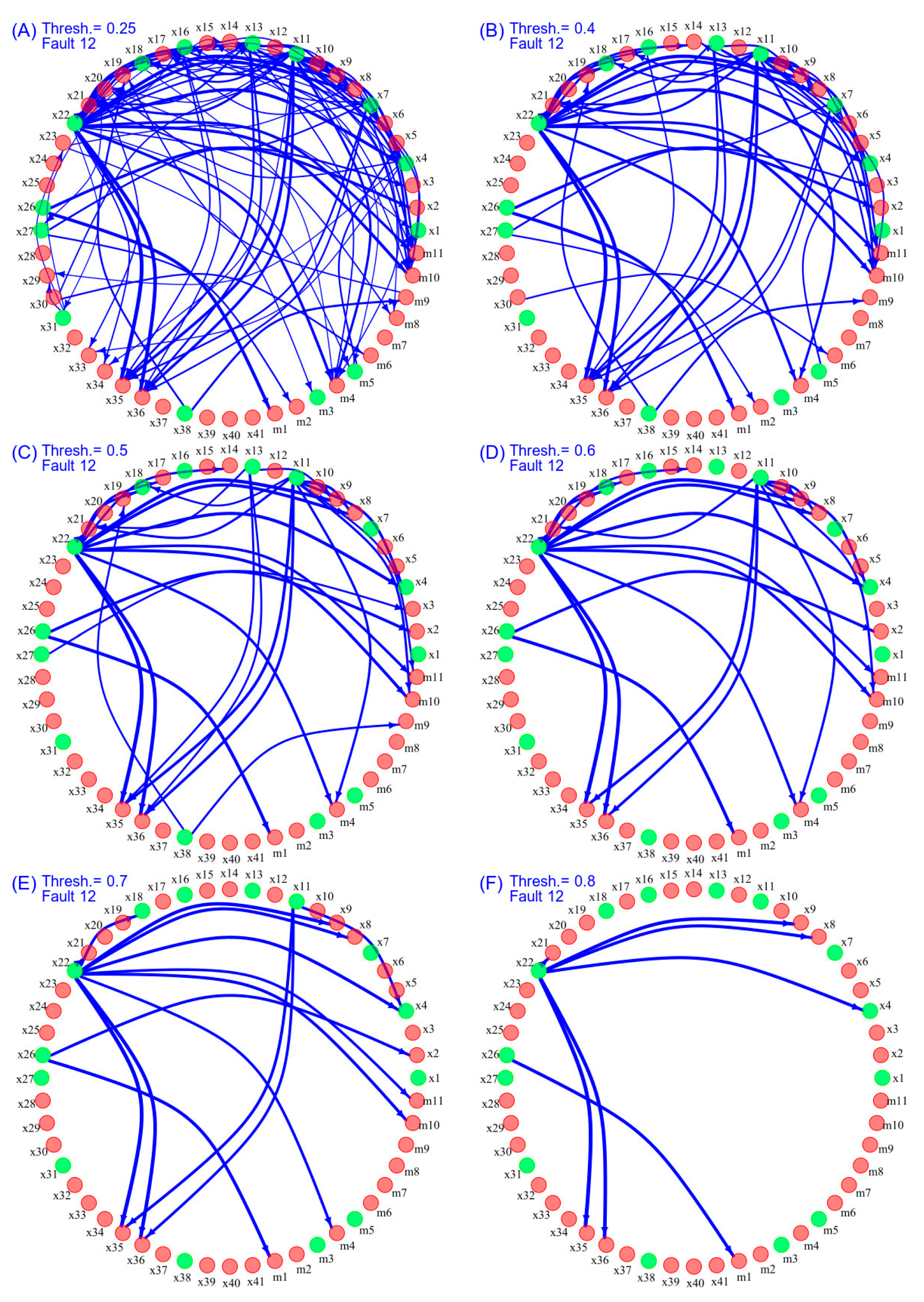
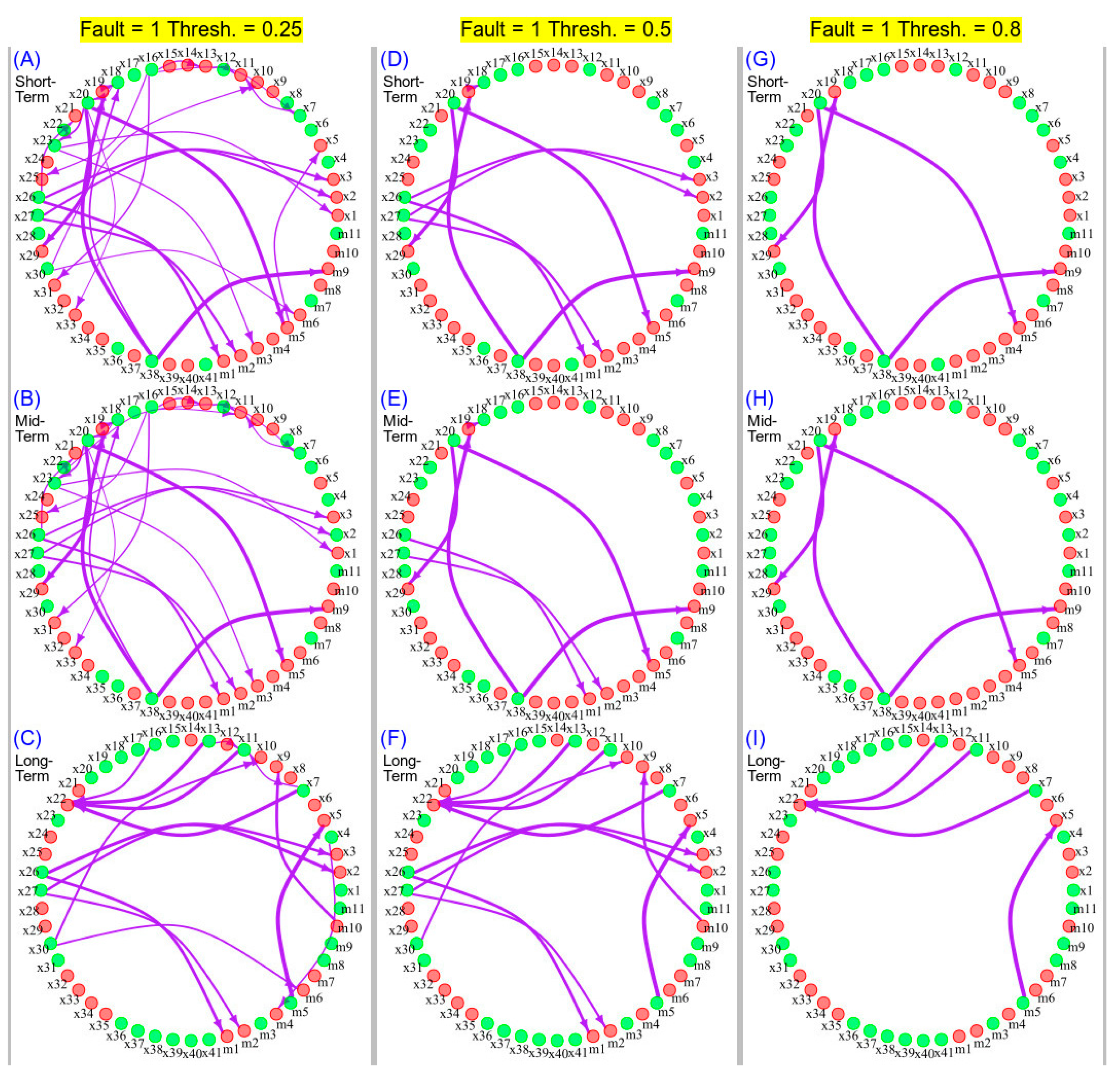
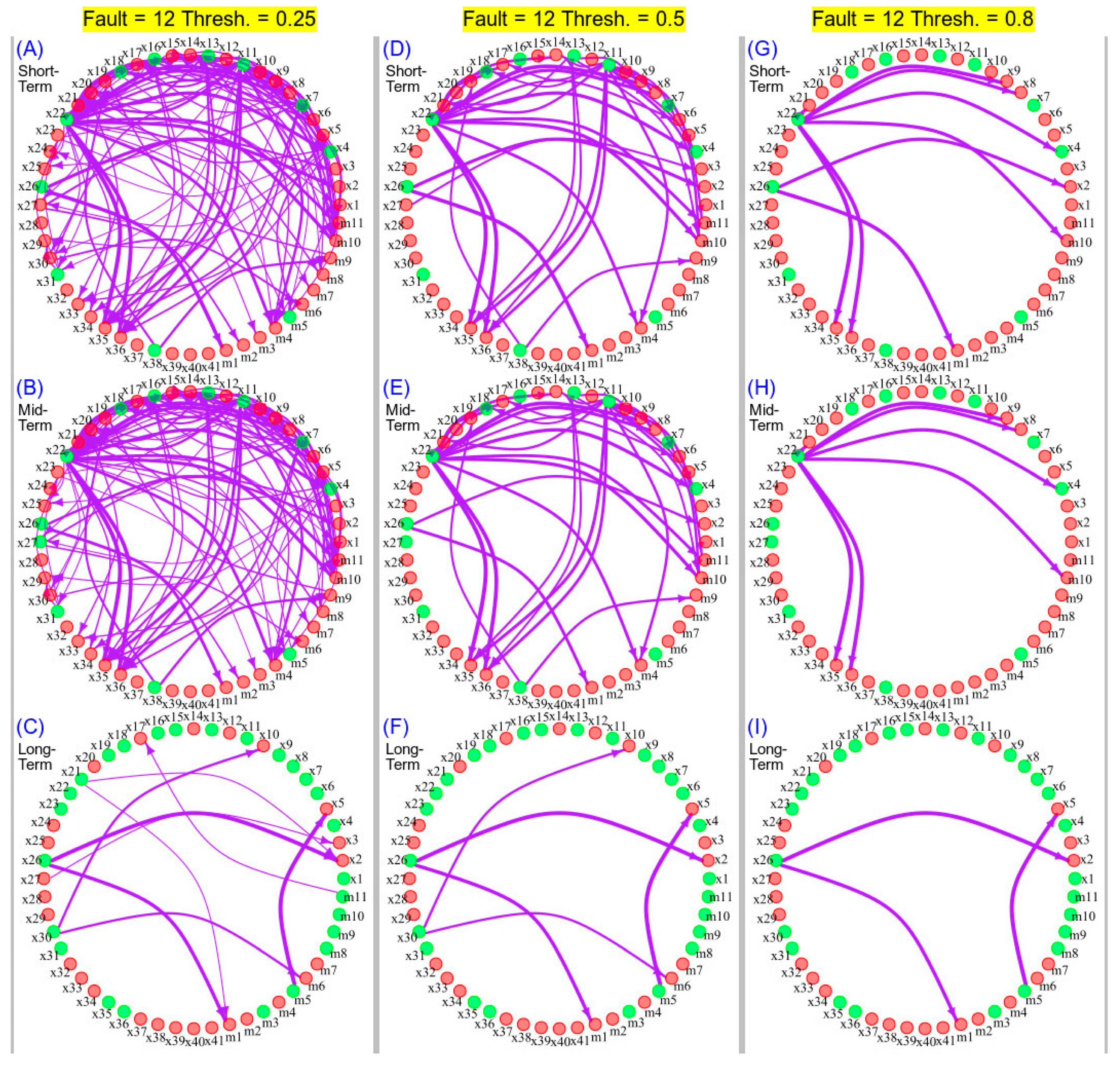
3.3. Network Topology at Varying Connectedness Thresholds

A question that naturally follows from the complicated network topology of Fault 12, as shown in Figure 7F, is the question of whether there is a way to segment the network topology based on the strength of the oscillation propagation effects (volatility index NPDC). The answer to the question is yes, and the sample solution for Fault 12 is shown in Figure 8. The solution is the set level of the minimum threshold of the volatility index NPDC to be considered for network rendering. That is, the NPDC index values greater than the set threshold fraction level will be the only NPDC index values to be considered for network topology rendering. For example, the maximum absolute value of the NPDC index in Fault 12 is 20.9 (see Figure A1 in Appendix A) and setting the threshold to 0.80 results in $20.9\times 0.80=16.72$ as the minimum NPDC value for network rendering resulting in Figure 8F, which has very few node connections but of high NPDC index values. These are the TEP process variables with high oscillation propagation effects in the system. If it is decided to add more node connections of lower NPDC values, i.e., in addition to the high NPDC node pairs, to expand the network analysis of oscillation, then the threshold can be set lower. This minimum threshold level then affects the number of visible node connections: the higher the minimum threshold, the higher the NPDC value cut-off resulting in fewer node connections that have high values of NPDC (Figure 8). There is no set rule about the level of the NPDC threshold, but the flexibility in varying this value as a means to add or remove the connections in the NPDC network allows for the possibility of prioritizing the process variables for further analysis of the oscillation propagation effects.

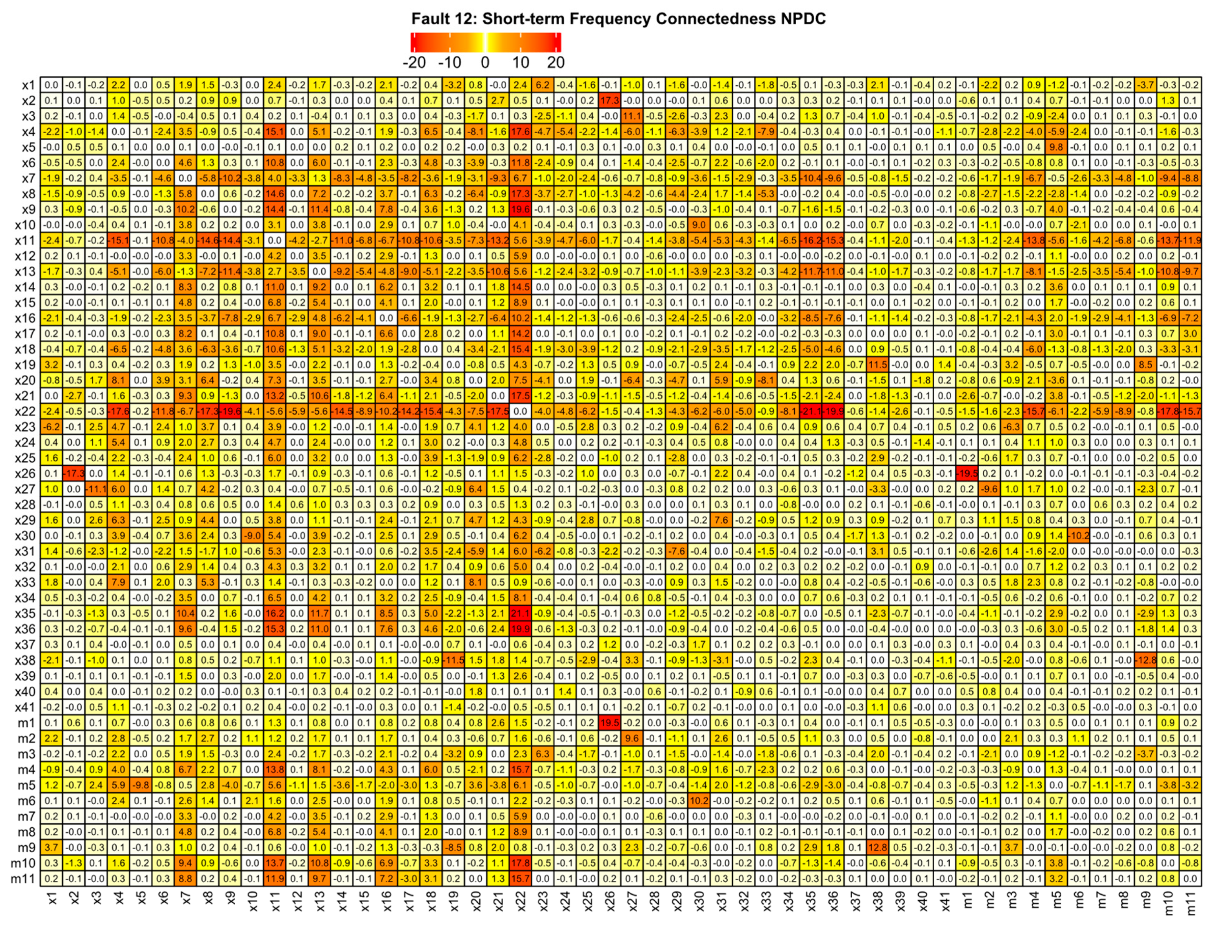
3.4. Connectedness Based on Frequency

Connectedness based on frequency may be a better model of connectedness when the time-series dynamics have a dominant periodic pattern [13]. Oscillations due to control loops is a challenging dynamics to detect and address in large-scale chemical processes [2]. Such periodic dynamics are apparent in the TEP dynamics, as shown in Figure 1 and Figure A1. Figure 9 and Figure 10 below show the network topology on the NPDC index based on frequency-connectedness $C_F$ at varying minimum threshold of the coefficients.

Apparent in both Fault 1 (Figure 9) and Fault 12 (Figure 10) are the differences in the network topology on the NPDC index between the short-term, mid-term, and long-term frequencies. In general, fewer oscillations are significant in long-term frequencies compared to short-term frequencies. This is expected in a system that has a control loop like the TEP, and it is an indication that the control loops are working to mitigate the disturbances arising from the faults.

For Fault 1 (Figure 9), the oscillation effects with high NPDC at a threshold of 0.8 at short-term are the following: the effect of x20 on x29 and m5; and the effect of x38 on x19 and m9 (Figure 9G). In the long-term, the following have high oscillation effects at the NPDC threshold of 0.8: x22 affected by x13, x11, and x7, and the effect of 5m to x5 (Figure 9I).

For Fault 12 (Figure 10), the oscillation effects with high NPDC at a threshold of 0.8 at short-term are the following: effect of x22 on x2, x4, x8, x9, x35, x36, and m10 (Figure 10G). In the long-term, the following have high oscillation effects at the NPDC threshold of 0.8: x26 on x2 and m1; and m5 on x5 (Figure 10I).

The connectedness index NPDC is significant in the short-term capture of the shock effects that occur and dissipate in short-term cyclical dynamics [13,24,25]. Hence, the oscillation connectedness at short-term measures the dynamics that rapidly manifest after a disturbance. On the other hand, the significant connectedness in the long-term capture the cyclical dynamics transmitted for long periods after a shock or disturbance [13,24,25]. Hence, the oscillation connectedness in the long term measure the dynamics that persist for a long time.

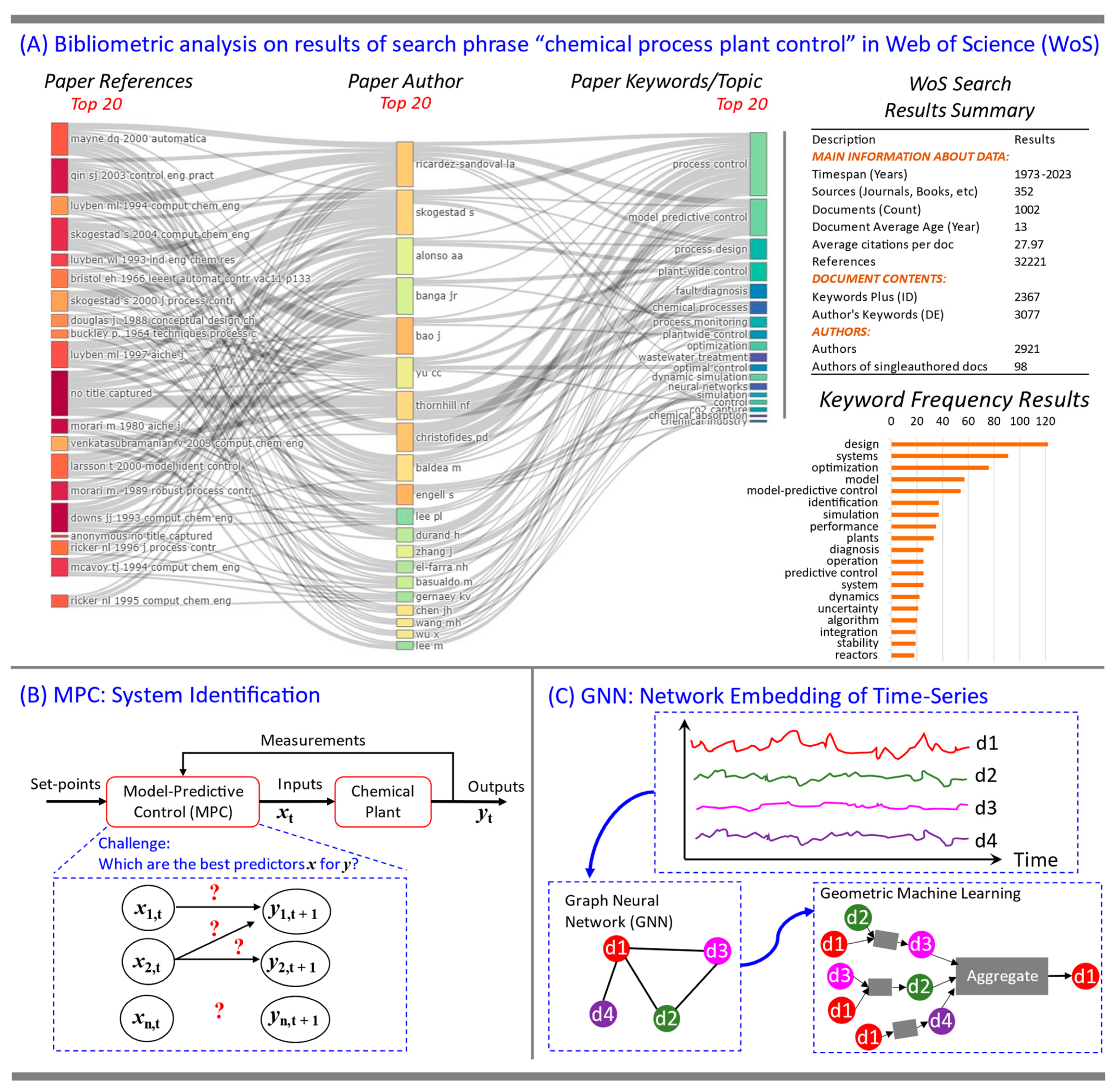
3.5. Significance of the Current Work

Chemical processes in small-scale or large-scale operations involve several control loops, and the corrective action of these control loops when a disturbance or fault occurs can result in oscillations propagating to many units through control loops and physical connections between units [2,26]. Hence, the disturbances may propagate to a plant-wide oscillation that can compromise product quality, increase the cost of operation, and increase the risk of accidents [1,4]. A recent review of literature conducted by Jiang and Yan [27] has identified that one of the key challenges in the plant-wide dynamics of the chemical process is the task of cause-effect and oscillation propagation path analysis. Capturing causality and connectivity has been a challenge for complex industrial-scale processes [28]. The demonstration in this work on the use of generalized variance decomposition to determine oscillation connectedness and the rendering of the NPDC volatility index as network graphs are aimed at introducing the said approach as an additional tool detecting and handling plant-wide oscillations caused by disturbances and faults.

Though the motivation of the work is to demonstrate a computational tool to detect oscillation propagation effects in a chemical process plant, the findings of the work may be of use in broader key areas of the field. We conducted a comprehensive literature review and bibliometric analysis to examine the state-of-art of the field of chemical process control and to show the significance of the current work. The results are summarized in Figure 11.

Figure 11A summarizes the results of bibliometric analysis on publications in Web of Science (WoS) on the search key phrase “chemical process plant control” for publication years 1973 to 2023. The top 1002 publications “by relevance” were collected and used in bibliometric analysis using the R-package “Bibliometrix” [29]. The three-field association plot in the form of a Sankey diagram for the top 20 authors, top 20 references, and top 20 topics depict the prominent research areas and researchers on the topic. The bibliographic dataset collected and the R-code for the analysis are provided in the online GitHub repository of the project [20]. It can be observed that the topic is averaging a publication of 13 documents per year from 352 sources (journals, books, etc.), and the average citation per document is 27.97. The topic of model-predictive control (MPC) is at the top of the list of topics, together with the topic area of neural networks (Figure 11A). These two topic areas fit well into the broader application of the results of this current work (Figure 11B,C).

Figure 11. Potential applications of the results of the network topology of oscillation propagation effects of disturbances and faults in a chemical process plant: (A) A comprehensive literature review and bibliometric analysis on the search key phrase “chemical process plant control” in the database Web of Science (WoS) for publication years 1973 to 2023. The top 1002 publications “by relevance” were collected and used in bibliometric analysis using the R-package “Bibliometrix”. A Sankey diagram of the Top 20 Author, Top 20 References, and Top 20 Topics represent a three-field summary of the top bibliometric entries in the 1002 publications. A frequency plot of keywords also provides a distribution of the prominent research terms. Top 20 authors: Ricardez-Sandoval [30], Skogestad [31], Alonso [32], Banga [33], Bao [34], Yu [35], Thornhill [36], Christofides [37], Baldea [38], Engell [39], Lee [40], Durand [41], Zhang [42], El-Farra [43], Basualdo [44], Gernaey [45], Chen [46], Wang [47], Wu [48], and Lee [49]. Top 20 references: Mayne [50], Qin [51], Luyben [52], Bristol [53], Skogestad [54], Douglas [55], Buckley [56], Luyben [57], Morari [58], Venkatasubramanian [59], Larsson [60], Morari [61], Downs [4], Ricker [62], McAvoy [63], and Ricker [64]. (B) Model-predictive control is an active research area particularly focused on the problem of system identification. (C) Graph-based machine learning of time-series datasets is also an active research area that can benefit from the network topology embedding of the time-series parameters.

Figure 11. Potential applications of the results of the network topology of oscillation propagation effects of disturbances and faults in a chemical process plant: (A) A comprehensive literature review and bibliometric analysis on the search key phrase “chemical process plant control” in the database Web of Science (WoS) for publication years 1973 to 2023. The top 1002 publications “by relevance” were collected and used in bibliometric analysis using the R-package “Bibliometrix”. A Sankey diagram of the Top 20 Author, Top 20 References, and Top 20 Topics represent a three-field summary of the top bibliometric entries in the 1002 publications. A frequency plot of keywords also provides a distribution of the prominent research terms. Top 20 authors: Ricardez-Sandoval [30], Skogestad [31], Alonso [32], Banga [33], Bao [34], Yu [35], Thornhill [36], Christofides [37], Baldea [38], Engell [39], Lee [40], Durand [41], Zhang [42], El-Farra [43], Basualdo [44], Gernaey [45], Chen [46], Wang [47], Wu [48], and Lee [49]. Top 20 references: Mayne [50], Qin [51], Luyben [52], Bristol [53], Skogestad [54], Douglas [55], Buckley [56], Luyben [57], Morari [58], Venkatasubramanian [59], Larsson [60], Morari [61], Downs [4], Ricker [62], McAvoy [63], and Ricker [64]. (B) Model-predictive control is an active research area particularly focused on the problem of system identification. (C) Graph-based machine learning of time-series datasets is also an active research area that can benefit from the network topology embedding of the time-series parameters.

3.5.1. Model-Predictive Control (MPC)—System Identification

The topic of MPC is a top research area where some of the prominent researchers in the field have conducted studies (Figure 11A) [31,32,37,65,66,67,68,69,70]. This is due to the potential of MPC to determine the optimal actions to take for large multi-input, multi-output (MIMO) systems [71]. Inherent in the implementation of MPC in a chemical plant, however, is the challenge of system identification (Figure 11B). System identification is the task of developing from process data the empirical models that become the “predictor” component of the MPC [72]. The MPC model must be efficient in capturing the relevant dynamics for a given objective [73]. The results of the connectedness measures from the generalized variance decomposition completed in this work can be used in identifying sets of predictor variables for specific target process output variables.

The interconnectedness of dynamics of various process variables depending on the fault (Figure 6 and Figure 7) elucidates whether the designated manipulated variables (m1, m2, … m11) are affecting the intended controlled variables (x1, x2, … x41) for that particular control loop. They also allow the detection of the spillover effects of manipulated variables onto controlled variables that are far downstream in the process. Such detection is difficult to do using only knowledge of first principles of mass balance, energy balance, kinetics and transfer phenomena because of the system-wide interconnectedness of the effects.

Another challenge that can be addressed by using the network topology of volatility spillover is the stratification of the spillover effects based on their levels. This is evident in the network topologies of NPDC at varying minimum thresholds (Figure 8). This allows for detecting which process variables must be prioritized for further analysis, as the high NPDC bivariate pairs represent the connections that transmit the greatest volatilities.

Analyzing oscillation propagation at short-term, mid-term, and long-term frequencies (Figure 9 and Figure 10) allows for the analysis of effects that manifest immediately (short-term) and those that persist for a longer period (long-term). An evident trend in Figure 9 and Figure 10 is that the oscillations propagation connectedness dissipates when going from short-term to long-term periods. This trend is consistent with the TEP process, which has various PID control loops designed to handle process faults and disturbances [4].

3.5.2. Graph Neural Network—Network Embedding of Time-Series

With the advent of machine learning techniques from shallow learning to deep learning, many studies developed anomaly-detection algorithms and architectures based on the training of machine learning models on large datasets [3,74,75]. This work does not attempt to provide an alternative computation approach. Rather, this work highlights another possible approach to representing the effects of faults and disturbances in a chemical process plant in a graph-based manner (Figure 11C). With the recognition of the capabilities of graph-based machine learning (geometric machine learning), there is an ongoing effort to discover ways of embedding time-series dynamics into network graphs where various attributes of the original time-series data can be represented as node attributes or edge attributes [76]. A recent review of the literature on the topic by Tjøstheim and Jullum [76] found that the common embedding approach is by using functional principal components analysis (PCA) [77], independent component analysis (ICA) [78], autoencoding [79], and self-organizing maps (SOM) [80]. A relatively new area of topological dynamics analysis (TDA) inspired by ideas from the pure mathematics of topology is being studied in terms of statical properties, and more work has to be carried out with TDA [76].

The network topologies graphically rendered in Figure 6, Figure 7, Figure 8, Figure 9 and Figure 10 are the kind of graphs that can be directly used as inputs into graph neural network (GNN) tensors and be processed via geometric machine learning. The attributes of the nodes and edges in the network topologies computed via time-based and frequency-based connectedness can all be embedded as network properties and be used in the machine learning computations allowing for more attributes captured from the original time-series dataset. These can be the next paths of research in this topic area. GNN has been a recent active area of research in systems involving connected data [81], and its extensive application in chemical process control merits consideration.

4. Conclusions

The method of generalized variance decomposition can estimate the connectedness of variables in a chemical processing system such as the Tennessee-Eastman process (TEP) based on time and based on dynamics frequency. Treating the time-based and frequency-based connectedness matrices as adjacency matrices and rendering the resulting net pairwise dynamic connectedness (NPDC) index of volatility results into network graphs that aid in the analysis of cause–effect relations of oscillations resulting from faults in a chemical process. The network topology of oscillations can be analyzed depending on the level of the NPDC volatility index. The frequency-based NPDC index network allows for the detection of short-term, mid-term, and long-term oscillation effects. The results of the current work may be applicable in broader areas of application, such as system identification in model-predictive control and graph-based machine learning of time-series dynamics.

References

1. Duan, P.; Chen, T.; Shah, S.L.; Yang, F. Methods for root cause diagnosis of plant-wide oscillations. AIChE J. 2014, 60, 2019–2034. [Google Scholar] [CrossRef]
2. Wang, Y.; Hu, X.; Zhou, S.; Ji, G. Oscillation Source Detection for Large-Scale Chemical Process with Interpretative Structural Model. In Information Technology and Intelligent Transportation Systems, Proceedings of the 2015 International Conference on Information Technology and Intelligent Transportation Systems ITITS 2015, Xi’an, China, 12–13 December 2015; Springer: Cham, Switzerland, 2017; pp. 441–451. [Google Scholar]
3. Rieth, C.A.; Amsel, B.D.; Tran, R.; Cook, M.B. Issues and Advances in Anomaly Detection Evaluation for Joint Human-Automated Systems. In Advances in Human Factors in Robots and Unmanned Systems, Proceedings of the AHFE 2017 International Conference on Human Factors in Robots and Unmanned Systems, Los Angeles, CA, USA, 17–21 July 2017; Springer International Publishing: Cham, Switzerland, 2018; Volume 8, pp. 52–63. [Google Scholar]
4. Downs, J.J.; Vogel, E.F. A plant-wide industrial process control problem. Comput. Chem. Eng. 1993, 17, 245–255. [Google Scholar] [CrossRef]
5. Cao, J.; Zhang, L.; Zheng, J.; Xia, C. An Integrated Approach to Oscillation Propagation Identification and Source Locating in Process Multi-loop Systems. Chin. J. Chem. Eng. 2011, 19, 999–1008. [Google Scholar] [CrossRef]
6. Bounoua, W.; Aftab, M.F.; Omlin, C.W.P. Controller Performance Monitoring: A Survey of Problems and a Review of Approaches from a Data-Driven Perspective with a Focus on Oscillations Detection and Diagnosis. Ind. Eng. Chem. Res. 2022, 61, 17735–17765. [Google Scholar] [CrossRef]
7. Granger, C.W.J. Investigating Causal Relations by Econometric Models and Cross-spectral Methods. Econometrica 1969, 37, 424–438. [Google Scholar] [CrossRef]
8. Stokes, P.A.; Purdon, P.L. A study of problems encountered in Granger causality analysis from a neuroscience perspective. Proc. Natl. Acad. Sci. USA 2017, 114, E7063–E7072. [Google Scholar] [CrossRef] [PubMed] [Green Version]
9. Shojaie, A.; Fox, E.B. Granger Causality: A Review and Recent Advances. arXiv 2021. [Google Scholar] [CrossRef]
10. Diebold, F.X.; Yılmaz, K. On the network topology of variance decompositions: Measuring the connectedness of financial firms. J. Econom. 2014, 182, 119–134. [Google Scholar] [CrossRef] [Green Version]
11. Jiang, W.; Gao, R.; Lu, C. The Analysis of Causality and Risk Spillover between Crude Oil and China’s Agricultural Futures. Int. J. Environ. Res. Public Health 2022, 19, 10593. [Google Scholar] [CrossRef]
12. Diebold, F.X.; Yilmaz, K. Financial and Macroeconomic Connectedness: A Network Approach to Measurement and Monitoring; Oxford University Press: Oxford, UK, 2015. [Google Scholar] [CrossRef]
13. Baruník, J.; Křehlík, T. Measuring the Frequency Dynamics of Financial Connectedness and Systemic Risk. J. Financ. Econom. 2018, 16, 271–296. [Google Scholar] [CrossRef]
14. Marlin, T.E. Process Control: Designing Processes and Control Systems for Dynamic Performance, 2nd ed.; McGraw-Hill Company: New York, NY, USA, 2000. [Google Scholar]
15. Joffe, M. Equilibrium, Instability, Growth and Feedback in Economics. In Feedback Economics: Economic Modeling with System Dynamics; Cavana, R.Y., Dangerfield, B.C., Pavlov, O.V., Radzicki, M.J., Wheat, I.D., Eds.; Springer International Publishing: Cham, Switzerland, 2021; pp. 43–68. [Google Scholar] [CrossRef]
16. Rieth, C.A.; Amsel, B.D.; Tran, R.; Cook, M.B. Additional Tennessee Eastman Process Simulation Data for Anomaly Detection Evaluation; Harvard Dataverse: Cambridge, MA, USA, 2017. [Google Scholar] [CrossRef]
17. Diebold, F.X.; Yilmaz, K. Measuring Financial Asset Return and Volatility Spillovers, with Application to Global Equity Markets. Econ. J. 2009, 119, 158–171. [Google Scholar] [CrossRef] [Green Version]
18. CRAN. The Comprehensive R Archive Network (CRAN); CRAN: Vienna, Austria, 2023. [Google Scholar]
19. RStudioTeam. RStudio: Integrated Development for R. RStudio; PBC: Boston, MA, USA, 2020. [Google Scholar]
20. Fortela, D.L.B.; Mikolajczyk, A.P. Tennessee-Eastman Chemical Process (TEP) Connectedness; GitHub: San Francisco, CA, USA, 2023. [Google Scholar]
21. Gabauer, D.; Gabauer, M.D. R-Package: ConnectednessApproach, R package Version 1.0.1; The Comprehensive R Archive Network (CRAN): Vienna, Austria, 2022. [Google Scholar]
22. Kang, S.H.; Lee, J.W. The network connectedness of volatility spillovers across global futures markets. Phys. A: Stat. Mech. Its Appl. 2019, 526, 120756. [Google Scholar] [CrossRef]
23. Csardi, G.; Nepusz, T. The igraph software package for complex network research. InterJournal 2006, 1695, 1–9. [Google Scholar]
24. Naeem, M.A.; Peng, Z.; Suleman, M.T.; Nepal, R.; Shahzad, S.J.H. Time and frequency connectedness among oil shocks, electricity and clean energy markets. Energy Econ. 2020, 91, 104914. [Google Scholar] [CrossRef]
25. Chatziantoniou, I.; Gabauer, D.; Gupta, R. Integration and Risk Transmission in the Market for Crude Oil: A Time-Varying Parameter Frequency Connectedness Approach; University of Pretoria, Department of Economics: Pretoria, South Africa, 2021. [Google Scholar]
26. Wu, W.; Song, C.; Liu, J.; Zhao, J. Data-knowledge-driven distributed monitoring for large-scale processes based on digraph. J. Process Control. 2022, 109, 60–73. [Google Scholar] [CrossRef]
27. Jiang, Q.; Yan, X.; Huang, B. Review and Perspectives of Data-Driven Distributed Monitoring for Industrial Plant-Wide Processes. Ind. Eng. Chem. Res. 2019, 58, 12899–12912. [Google Scholar] [CrossRef]
28. Yang, F.; Duan, P.; Shah, S.L.; Chen, T. Capturing Causality from Process Data. In Capturing Connectivity and Causality in Complex Industrial Processes; Yang, F., Duan, P., Shah, S.L., Chen, T., Eds.; Springer International Publishing: Cham, Switzerland, 2014; pp. 41–65. [Google Scholar] [CrossRef]
29. Aria, M.; Cuccurullo, C. Bibliometrix: An R-tool for comprehensive science mapping analysis. J. Informetr. 2017, 11, 959–975. [Google Scholar] [CrossRef]
30. Ricardez-Sandoval, L.A.; Budman, H.M.; Douglas, P.L. Simultaneous design and control of chemical processes with application to the Tennessee Eastman process. J. Process Control 2009, 19, 1377–1391. [Google Scholar] [CrossRef]
31. Skogestad, S. Control structure design for complete chemical plants. Comput. Chem. Eng. 2004, 28, 219–234. [Google Scholar] [CrossRef]
32. Antelo, L.T.; Banga, J.R.; Alonso, A.A. Hierarchical design of decentralized control structures for the Tennessee Eastman Process. Comput. Chem. Eng. 2008, 32, 1995–2015. [Google Scholar] [CrossRef]
33. Antelo, L.T.; Exler, O.; Banga, J.R.; Alonso, A.A. Optimal tuning of thermodynamic-based decentralized PI control loops: Application to the Tennessee Eastman Process. AIChE J. 2008, 54, 2904–2924. [Google Scholar] [CrossRef] [Green Version]
34. Tippett, M.J.; Bao, J. Distributed model predictive control based on dissipativity. AIChE J. 2012, 59, 787–804. [Google Scholar] [CrossRef]
35. Lin, S.-W.; Yu, C.-C. Design and control for recycle plants with heat-integrated separators. Chem. Eng. Sci. 2004, 59, 53–70. [Google Scholar] [CrossRef]
36. Thornhill, N. Finding the source of nonlinearity in a process with plant-wide oscillation. IEEE Trans. Control. Syst. Technol. 2005, 13, 434–443. [Google Scholar] [CrossRef] [Green Version]
37. Durand, H.; Christofides, P.D. Economic Model Predictive Control: Handling Valve Actuator Dynamics and Process Equipment Considerations. Found. Trends® Syst. Control. 2018, 5, 293–350. [Google Scholar] [CrossRef]
38. Baldea, M.; El-Farra, N.H.; Ydstie, B.E. Dynamics and control of chemical process networks: Integrating physics, communication and computation. Comput. Chem. Eng. 2012, 51, 42–54. [Google Scholar] [CrossRef]
39. Engell, S. Feedback control for optimal process operation. J. Process. Control. 2007, 17, 203–219. [Google Scholar] [CrossRef]
40. Nott, H.; Lee, P. An optimal control approach for scheduling mixed batch/continuous process plants with variable cycle time. Comput. Chem. Eng. 1999, 23, 907–917. [Google Scholar] [CrossRef]
41. Durand, H. A Nonlinear Systems Framework for Cyberattack Prevention for Chemical Process Control Systems. Mathematics 2018, 6, 169. [Google Scholar] [CrossRef] [Green Version]
42. Li, C.; Zhang, J.; Wang, G. Batch-to-batch optimal control of batch processes based on recursively updated nonlinear partial least squares models. Chem. Eng. Commun. 2006, 194, 261–279. [Google Scholar] [CrossRef]
43. El-Farra, N.H.; Gani, A.; Christofides, P.D. Fault-tolerant control of process systems using communication networks. AIChE J. 2005, 51, 1665–1682. [Google Scholar] [CrossRef]
44. Zumoffen, D.; Basualdo, M. From Large Chemical Plant Data to Fault Diagnosis Integrated to Decentralized Fault-Tolerant Control: Pulp Mill Process Application. Ind. Eng. Chem. Res. 2008, 47, 1201–1220. [Google Scholar] [CrossRef]
45. Ingildsen, P.; Rosen, C.; Gernaey, K.; Nielsen, M.; Guildal, T.; Jacobsen, B. Modelling and control strategy testing of biological and chemical phosphorus removal at Avedøre WWTP. Water Sci. Technol. 2006, 53, 105–113. [Google Scholar] [CrossRef] [PubMed]
46. Chan, L.L.T.; Chen, J. Probabilistic uncertainty based simultaneous process design and control with iterative expected improvement model. Comput. Chem. Eng. 2017, 106, 609–620. [Google Scholar] [CrossRef]
47. Biliyok, C.; Lawal, A.; Wang, M.; Seibert, F. Dynamic modelling, validation and analysis of post-combustion chemical absorption CO2 capture plant. Int. J. Greenh. Gas Control. 2012, 9, 428–445. [Google Scholar] [CrossRef]
48. Wu, X.; Shen, J.; Li, Y.; Wang, M.; Lawal, A.; Lee, K.Y. Nonlinear dynamic analysis and control design of a solvent-based post-combustion CO2 capture process. Comput. Chem. Eng. 2018, 115, 397–406. [Google Scholar] [CrossRef]
49. Husnil, Y.A.; Lee, M. Control structure synthesis for operational optimization of mixed refrigerant processes for liquefied natural gas plant. AIChE J. 2014, 60, 2428–2441. [Google Scholar] [CrossRef]
50. Mayne, D.Q. Model predictive control: Recent developments and future promise. Automatica 2014, 50, 2967–2986. [Google Scholar] [CrossRef]
51. Qin, S.; Badgwell, T.A. A survey of industrial model predictive control technology. Control. Eng. Pract. 2002, 11, 733–764. [Google Scholar] [CrossRef]
52. Luyben, M.; Floudas, C. Analyzing the interaction of design and control—1. A multiobjective framework and application to binary distillation synthesis. Comput. Chem. Eng. 1994, 18, 933–969. [Google Scholar] [CrossRef]
53. Bristol, E. On a new measure of interaction for multivariable process control. IEEE Trans. Autom. Control 1966, 11, 133–134. [Google Scholar] [CrossRef]
54. Skogestad, S. Plantwide control: The search for the self-optimizing control structure. J. Process. Control. 2000, 10, 487–507. [Google Scholar] [CrossRef]
55. Douglas, J.M. Conceptual Design of Chemical Processes; McGraw-Hill: New York, NY, USA, 1988; p. 601. [Google Scholar]
56. Buckley, P.S. Techniques of Process Control; Wiley: Hoboken, NJ, USA, 1965. [Google Scholar]
57. Luyben, M.L.; Tyréus, B.D. An industrial design/control study for the vinyl acetate monomer process. Comput. Chem. Eng. 1998, 22, 867–877. [Google Scholar] [CrossRef]
58. Morari, M.; Stephanopoulos, G. Studies in the synthesis of control structures for chemical processes: Part II: Structural aspects and the synthesis of alternative feasible control schemes. AIChE J. 1980, 26, 232–246. [Google Scholar] [CrossRef]
59. Venkatasubramanian, V.; Rengaswamy, R.; Yin, K.; Kavuri, S.N. A review of process fault detection and diagnosis: Part I: Quantitative model-based methods. Comput. Chem. Eng. 2003, 27, 293–311. [Google Scholar] [CrossRef]
60. Truls, L.; Skogestad, S. Plantwide control—A review and a new design procedure. Model. Identif. Control 2000, 21, 209–240. [Google Scholar]
61. Morari, M.; Zafiriou, E. Robust Process Control; Prentice-Hall, Inc.: Englewood Cliffs, NJ, USA, 1989; p. 488. [Google Scholar]
62. Ricker, N.L. Decentralized control of the Tennessee Eastman Challenge Process. J. Process. Control. 1996, 6, 205–221. [Google Scholar] [CrossRef]
63. McAvoy, T.; Ye, N. Base control for the Tennessee Eastman problem. Comput. Chem. Eng. 1994, 18, 383–413. [Google Scholar] [CrossRef]
64. Ricker, N.; Lee, J. Nonlinear model predictive control of the Tennessee Eastman challenge process. Comput. Chem. Eng. 1995, 19, 961–981. [Google Scholar] [CrossRef]
65. Bahakim, S.S.; Ricardez-Sandoval, L.A. Simultaneous design and MPC-based control for dynamic systems under uncertainty: A stochastic approach. Comput. Chem. Eng. 2014, 63, 66–81. [Google Scholar] [CrossRef]
66. Gutierrez, G.; Ricardez-Sandoval, L.A.; Budman, H.; Prada, C. An MPC-based control structure selection approach for simultaneous process and control design. Comput. Chem. Eng. 2014, 70, 11–21. [Google Scholar] [CrossRef]
67. He, Z.R.; Sahraei, M.H.; Ricardez-Sandoval, L.A. Flexible operation and simultaneous scheduling and control of a CO2 capture plant using model predictive control. Int. J. Greenh. Gas Control 2016, 48, 300–311. [Google Scholar] [CrossRef]
68. Francisco, M.; Skogestad, S.; Vega, P. Model predictive control for the self-optimized operation in wastewater treatment plants: Analysis of dynamic issues. Comput. Chem. Eng. 2015, 82, 259–272. [Google Scholar] [CrossRef] [Green Version]
69. Albalawi, F.; Durand, H.; Christofides, P.D. Process operational safety via model predictive control: Recent results and future research directions. Comput. Chem. Eng. 2018, 114, 171–190. [Google Scholar] [CrossRef]
70. Wang, S.; Simkoff, J.M.; Baldea, M.; Chiang, L.H.; Castillo, I.; Bindlish, R.; Stanley, D.B. Autocovariance-based plant-model mismatch estimation for linear model predictive control. Syst. Control Lett. 2017, 104, 5–14. [Google Scholar] [CrossRef] [Green Version]
71. Forbes, M.G.; Patwardhan, R.S.; Hamadah, H.; Gopaluni, R.B. Model Predictive Control in Industry: Challenges and Opportunities. IFAC-Pap. 2015, 48, 531–538. [Google Scholar] [CrossRef]
72. Ortiz Torres, G.; Rumbo Morales, J.Y.; Ramos Martinez, M.; Valdez-Martínez, J.S.; Calixto-Rodriguez, M.; Sarmiento-Bustos, E.; Torres Cantero, C.A.; Buenabad-Arias, H.M. Active Fault-Tolerant Control Applied to a Pressure Swing Adsorption Process for the Production of Bio-Hydrogen. Mathematics 2023, 11, 1129. [Google Scholar] [CrossRef]
73. Kaiser, E.; Kutz, J.N.; Brunton, S.L. Sparse identification of nonlinear dynamics for model predictive control in the low-data limit. Proc. R. Soc. A Math. Phys. Eng. Sci. 2018, 474, 20180335. [Google Scholar] [CrossRef] [Green Version]
74. Lomov, I.; Lyubimov, M.; Makarov, I.; Zhukov, L.E. Fault detection in Tennessee Eastman process with temporal deep learning models. J. Ind. Inf. Integr. 2021, 23, 100216. [Google Scholar] [CrossRef]
75. Fabian Hartung, B.J.F.; Michels, T.; Wagner, D.; Liznerski, P.; Reithermann, S.; Fellenz, S.; Jirasek, F.; Rudolph, M.; Neider, D.; Leitte, H.; et al. Deep Anomaly Detection on Tennessee Eastman Process Data. arXiv 2023. [Google Scholar] [CrossRef]
76. Tjøstheim, D.; Jullum, M.; Løland, A. Some recent trends in embeddings of time series and dynamic networks. arXiv 2022. [Google Scholar] [CrossRef]
77. Peña, D.; Yohai, V.J. Generalized Dynamic Principal Components. J. Am. Stat. Assoc. 2016, 111, 1121–1131. [Google Scholar] [CrossRef]
78. Hyvärinen, A.; Oja, E. Independent component analysis: Algorithms and applications. Neural Netw. 2000, 13, 411–430. [Google Scholar] [CrossRef] [Green Version]
79. Hinton, G.E.; Salakhutdinov, R. Reducing the Dimensionality of Data with Neural Networks. Science 2006, 313, 504–507. [Google Scholar] [CrossRef] [PubMed] [Green Version]
80. Kohonen, T. Self-organized formation of topologically correct feature maps. Biol. Cybern. 1982, 43, 59–69. [Google Scholar] [CrossRef]
81. Xia, F.; Sun, K.; Yu, S.; Aziz, A.; Wan, L.; Pan, S.; Liu, H. Graph Learning: A Survey. IEEE Trans. Artif. Intell. 2021, 2, 109–127. [Google Scholar] [CrossRef]
Figure 1. P&ID rendering of the Tennessee-Eastman chemical process benchmark originally proposed by Downs and Vogel [4]. Number annotations denote stream number. Arrowed solid lines indicate flow stream direction. Dashed lines indicate signals of a control loop. Letters: FC = flow controller, FI = flow indicator, TC = temperature controller, TI = temperature indicator, LC = level controller, LI = liquid indicator, PI = pressure indicator, composition symbols: xA, xB, xC, xD, xE, xF, xG, and xH in mole fraction for chemical components A, B, C, D, E, F, G, and H, respectively. Valves are manipulated variables indicated by m1, m2, m3, etc.
Processes 11 01747 g001
Figure 2. A schematic depicting the analogy of feedback control loops (A) in chemical processing [14] and (B) in economic systems such as price-demand-supply dynamics [15].
Processes 11 01747 g002
Figure 3. Sample time-series dynamics of TEP with “Fault 1”, which is a negative step change of (x4) feed ratio of mol A/mol C in stream 4. The valve opening m3 compensated for increasing the feed flow of A (x1). The levels of the measured variables (x1 to x41) and the manipulated variables (m1 to m11) were sampled every 3 min.
Processes 11 01747 g003
Figure 4. Sample rendering of a toy example-directed network graph R from its corresponding adjacency matrix: (A) network weighted adjacency matrix and (B) network graph.
Processes 11 01747 g004
Figure 5. Data analysis workflow implemented for the TEP benchmark dataset.
Processes 11 01747 g005
Figure 6. Network topology of volatility spillover index net pairwise dynamic connectedness (NPDC) based on time-connectedness on Fault 1 to Fault 6 of the TEP. The NPDC threshold is 0.25. Nodes filled with green color have zero overall NPDC, while nodes filled with red color have positive overall NPDC. The arrowed edges indicate the direction of volatility spillover.
Processes 11 01747 g006
Figure 7. Network topology of volatility spillover index net pairwise dynamic connectedness (NPDC) based on time-connectedness on Fault 7 to Fault 12 of the TEP. The NPDC threshold is 0.25. Nodes filled with green color have zero overall NPDC, while nodes filled with red color have positive overall NPDC. The arrowed edges indicate the direction of volatility spillover.
Processes 11 01747 g007
Figure 8. Network topology of volatility spillover index net pairwise dynamic connectedness (NPDC) based on time-connectedness on Fault 12 at a varying minimum threshold of the NPDC. Nodes filled with green color have zero overall NPDC, while nodes filled with red color have positive overall NPDC. The arrowed edges indicate the direction of volatility spillover.
Processes 11 01747 g008
Figure 9. Network topology of volatility spillover index net pairwise dynamic connectedness (NPDC) based on frequency-connectedness on Fault 1 at a varying minimum threshold of the NPDC. Nodes filled with green color have zero overall NPDC, while nodes filled with red color have positive overall NPDC. The arrowed edges indicate the direction of volatility spillover.
Processes 11 01747 g009
Figure 10. Network topology of volatility spillover index net pairwise dynamic connectedness (NPDC) based on frequency-connectedness on Fault 12 at a varying minimum threshold of the NPDC. Nodes filled with green color have zero overall NPDC, while nodes filled with red color have positive overall NPDC. The arrowed edges indicate the direction of volatility spillover.
Processes 11 01747 g010