

Data-Driven Operation of Flexible Distribution Networks with Charging Loads
 and
and
Abstract
:1. Introduction
2. Framework of Data-Driven Operation of FDNs with Charging Loads
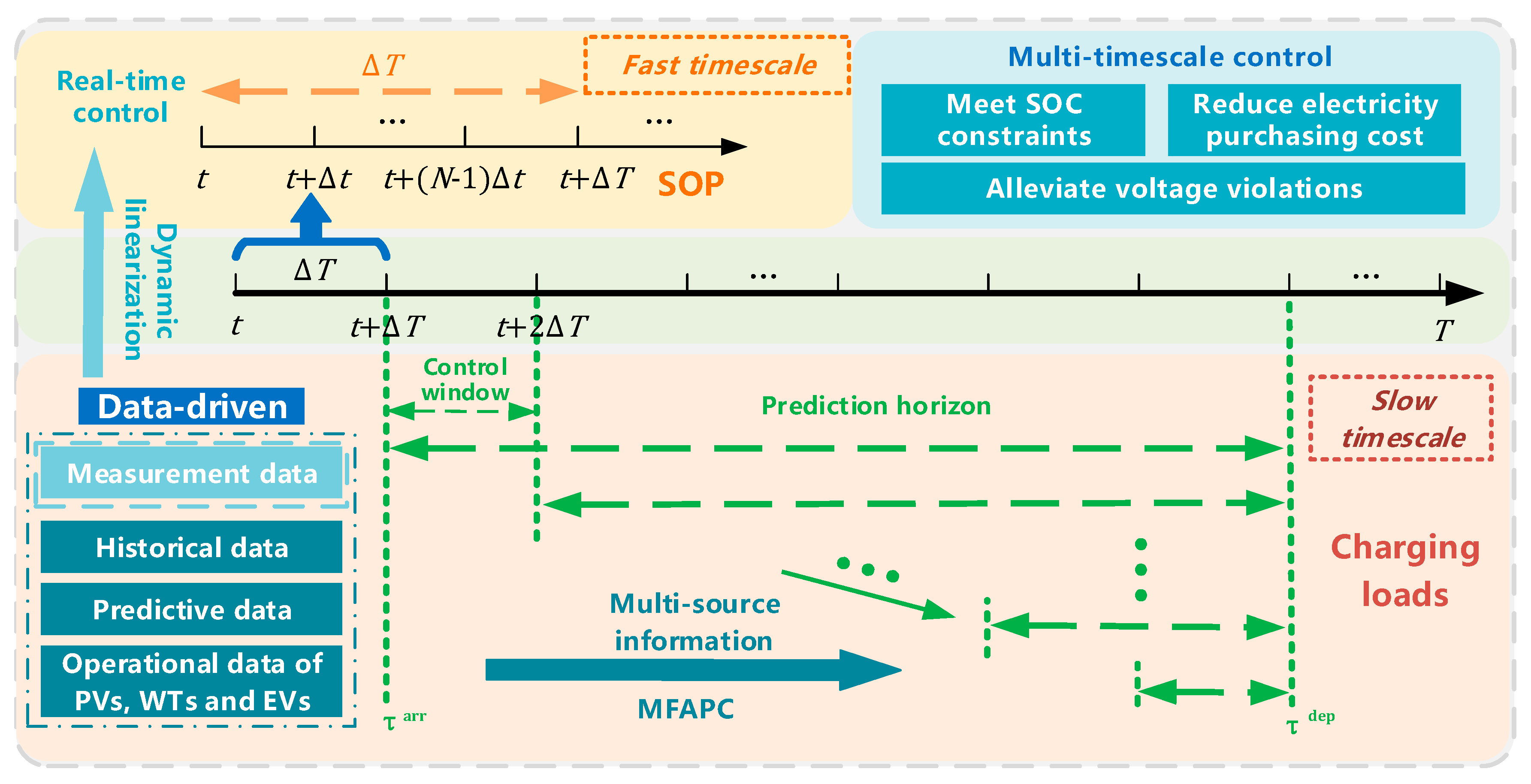
3. Multi-Timescale Data-Driven Operation Based on MFAPC
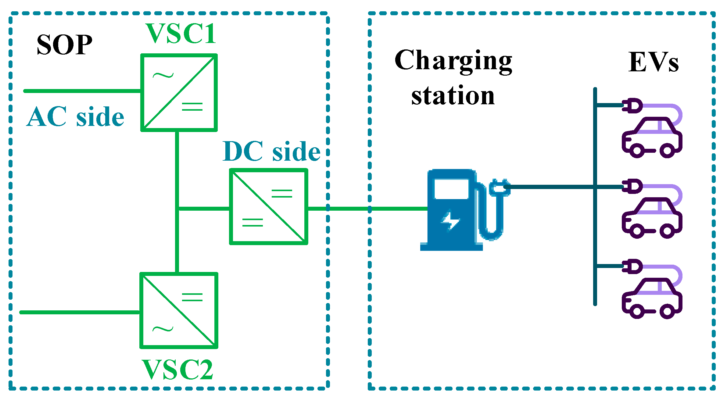
3.1. Data-Driven Operation Model of FDNs with Charging Loads
3.2. Multi-Timescale Coordination Control Model
3.3. Solution Methodology
4. Case Studies and Analysis
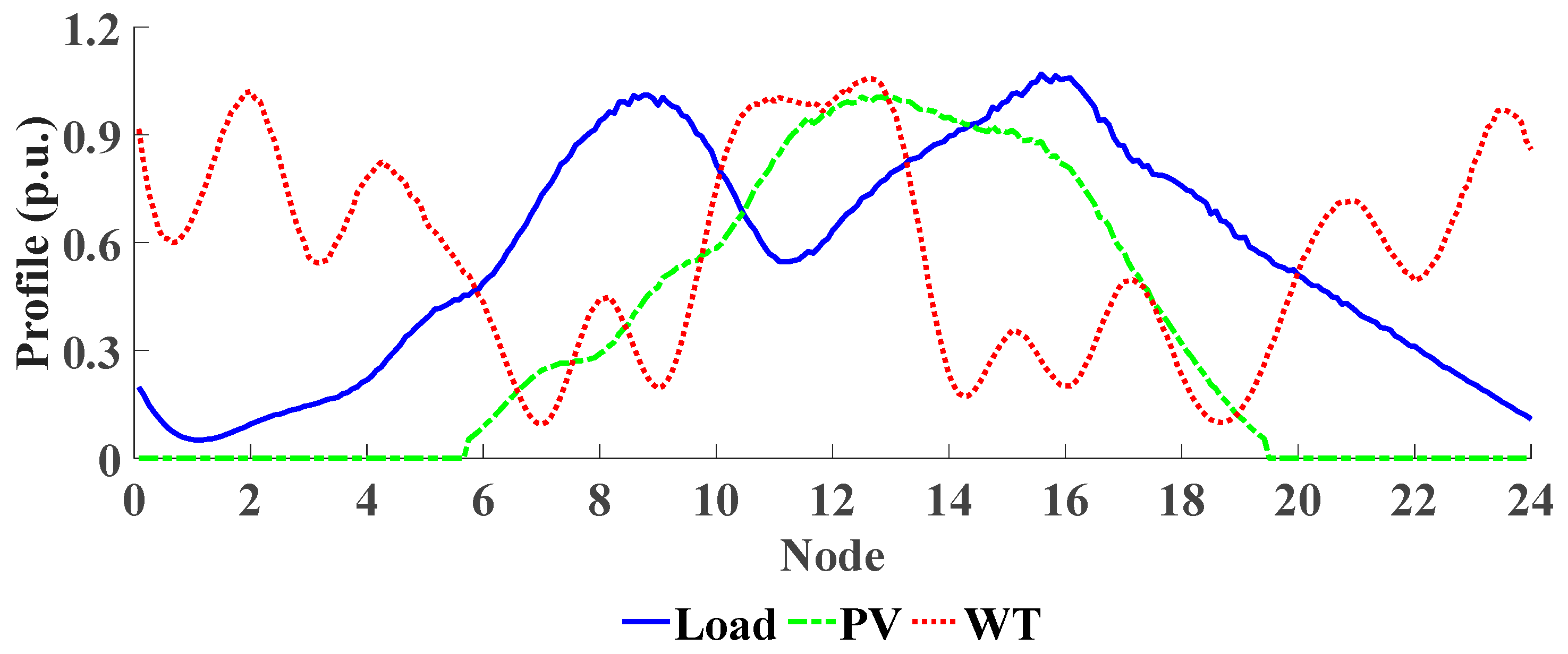
4.1. Parameters
4.2. Numerical Results
5. Conclusions
Author Contributions
Funding
Informed Consent Statement
Data Availability Statement
Conflicts of Interest
References
- Zhang, Y.; Yang, Y.; Zhang, X.; Pu, W.; Song, H. Planning strategies for distributed pv-storage using a distribution network based on load time sequence characteristics partitioning. Processes 2023, 11, 540. [Google Scholar] [CrossRef]
- Maghami, M.R.; Pasupuleti, J.; Ling, C.M. A static and dynamic analysis of photovoltaic penetration into MV distribution network. Processes 2023, 11, 1172. [Google Scholar] [CrossRef]
- Xiao, J.; Wang, Y.; Luo, F.; Bai, L.; Gang, F.; Huang, R.; Jiang, X.; Zhang, X. Flexible distribution network: Definition, configuration, operation, and pilot project. IET Gener. Transm. Distrib. 2018, 12, 4492–4498. [Google Scholar] [CrossRef]
- Ji, H.; Wang, C.; Li, P.; Ding, F.; Wu, J. Robust operation of soft open points in active distribution networks with high penetration of photovoltaic integration. IEEE Trans. Sustain. Energy 2019, 10, 280–289. [Google Scholar] [CrossRef]
- Ding, T.; Wang, Z.; Jia, W.; Chen, B.; Chen, C.; Shahidehpour, M. Multiperiod distribution system restoration with routing repair crews, mobile electric vehicles, and soft-open-point networked microgrids. IEEE Trans. Smart Grid 2020, 11, 4795–4808. [Google Scholar] [CrossRef]
- Xu, J.; Huang, Y. The short-term optimal resource allocation approach for electric vehicles and V2G service stations. Appl. Energy 2022, 319, 119200. [Google Scholar] [CrossRef]
- Mehta, R.; Srinivasan, D.; Trivedi, A.; Yang, J. Hybrid planning method based on cost-benefit analysis for smart charging of plug-in electric vehicles in distribution systems. IEEE Trans. Smart Grid 2019, 10, 523–534. [Google Scholar] [CrossRef]
- Wang, J.; Zhou, N.; Wang, Q.; Liu, H. Hierarchically coordinated optimization of power distribution systems with soft open points and electric vehicles. Int. J. Electr. Power Energy Syst. 2023, 149, 109040. [Google Scholar] [CrossRef]
- Maulik, A. Probabilistic power management of a grid-connected microgrid considering electric vehicles, demand response, smart transformers, and soft open points. Sustain. Energy Grids Netw. 2022, 30, 100636. [Google Scholar]
- Sun, X.; Qiu, J. A customized voltage control strategy for electric vehicles in distribution networks with reinforcement learning method. IEEE Trans. Industr. Inform. 2021, 17, 6852–6863. [Google Scholar] [CrossRef]
- Zhu, H.; Zhang, D.; Goh, H.H.; Wang, S.; Ahmad, T.; Mao, D.; Liu, T.; Zhao, H.; Wu, T. Future data center energy-conservation and emission-reduction technologies in the context of smart and low-carbon city construction. Sustain. Cities Soc. 2023, 89, 104322. [Google Scholar] [CrossRef]
- Tong, L.; Zhao, S.; Jiang, H.; Zhou, J.; Xu, B. Multi-scenario and multi-objective collaborative optimization of distribution network considering electric vehicles and mobile energy storage systems. IEEE Access 2021, 9, 55690–55697. [Google Scholar] [CrossRef]
- Zhu, X.; Han, H.; Gao, S.; Shi, Q.; Cui, H.; Zu, G. A multi-stage optimization approach for active distribution network scheduling considering coordinated electrical vehicle charging strategy. IEEE Access 2018, 6, 50117–50130. [Google Scholar] [CrossRef]
- Li, H.; Azzouz, M.A.; Hamad, A.A. Cooperative voltage control in MV distribution networks with electric vehicle charging stations and photovoltaic DGs. IEEE Syst. J. 2021, 15, 2989–3000. [Google Scholar] [CrossRef]
- Huo, Y.; Li, P.; Ji, H.; Yu, H.; Yan, J.; Wu, J.; Wang, C. Data-driven coordinated voltage control method of distribution networks with high DG penetration. IEEE Trans. Power Syst. 2023, 38, 1543–1557. [Google Scholar] [CrossRef]
- Lee, Z.J.; Sharma, S.; Johansson, D.; Low, S.H. ACN-Sim: An open-source simulator for data-driven electric vehicle charging research. IEEE Trans. Smart Grid 2021, 12, 5113–5123. [Google Scholar] [CrossRef]
- Khemmook, P.; Prompinit, K.; Surinkaew, T. Control of a microgrid using robust data-driven-based controllers of distributed electric vehicles. Electr. Power Syst. Res. 2022, 213, 108681. [Google Scholar] [CrossRef]
- Zhang, X.; Kong, X.; Yan, R.; Liu, Y.; Xia, P.; Sun, X.; Zeng, R.; Li, H. Data-driven cooling, heating and electrical load prediction for building integrated with electric vehicles considering occupant travel behavior. Energy 2023, 264, 126274. [Google Scholar] [CrossRef]
- Tao, Y.; Qiu, J.; Lai, S. A data-driven management strategy of electric vehicles and thermostatically controlled loads based on modified generative adversarial network. IEEE Trans. Transp. Electrif. 2022, 8, 1430–1444. [Google Scholar] [CrossRef]
- Wang, S.; Li, J.; Hou, Z.; Meng, Q.; Li, M. Composite model-free adaptive predictive control for wind power generation based on full wind speed. CSEE J. Power Energy Syst. 2022, 8, 1659–1669. [Google Scholar]
- Wang, Y.; Hou, Z. Event-triggered model-free adaptive predictive control for nonlinear NCSs with data dropout and application in PMSM control system. In Proceedings of the 2022 IEEE 11th Data Driven Control and Learning Systems Conference (DDCLS), Chengdu, China, 13–15 May 2022; pp. 1111–1117. [Google Scholar]
- Zhang, S.; Fang, Y.; Zhang, H.; Cheng, H.; Wang, X. Maximum hosting capacity of photovoltaic generation in SOP-based power distribution network integrated with electric vehicles. IEEE Trans. Industr. Inform. 2022, 18, 8213–8224. [Google Scholar] [CrossRef]


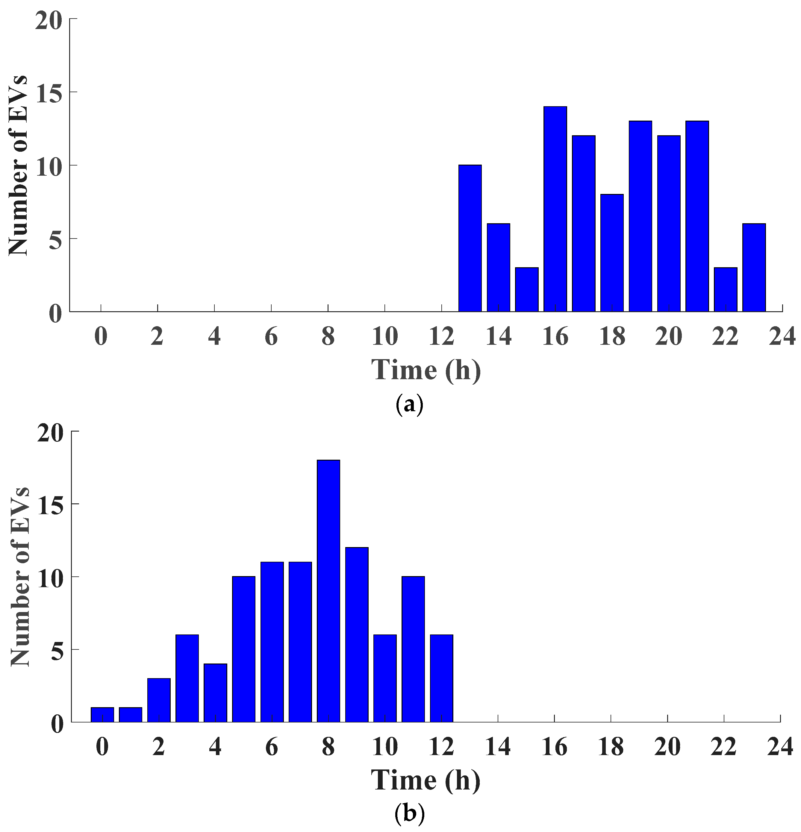
| Behaviors | Distribution |
|---|---|
| Arrival time | N (17.47, 6) |
| Departure time | N (8.92, 3.25) |
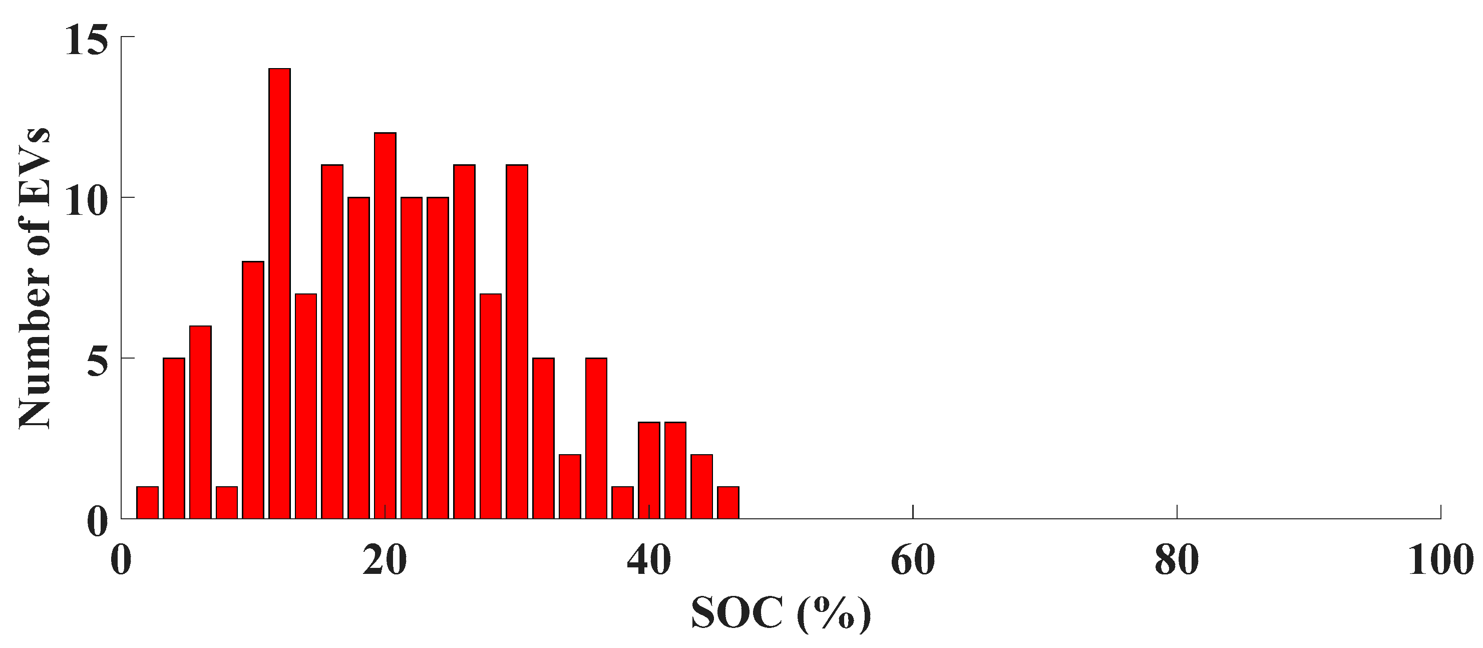
| Initial SOC | N (0.196, 0.1182) |
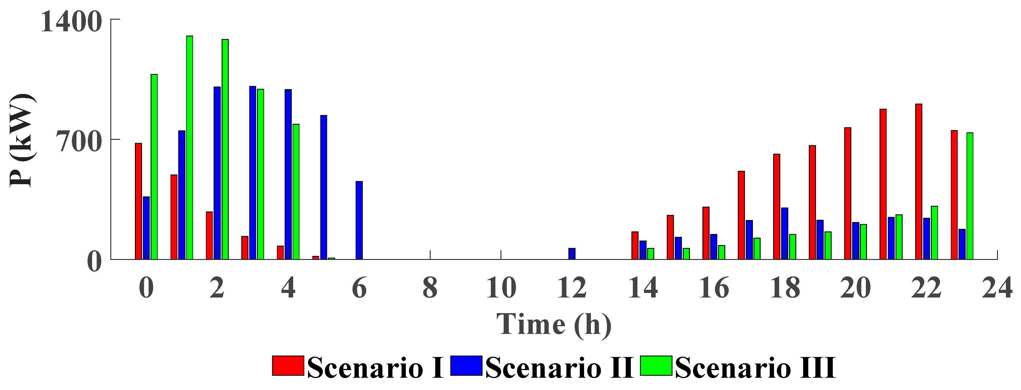
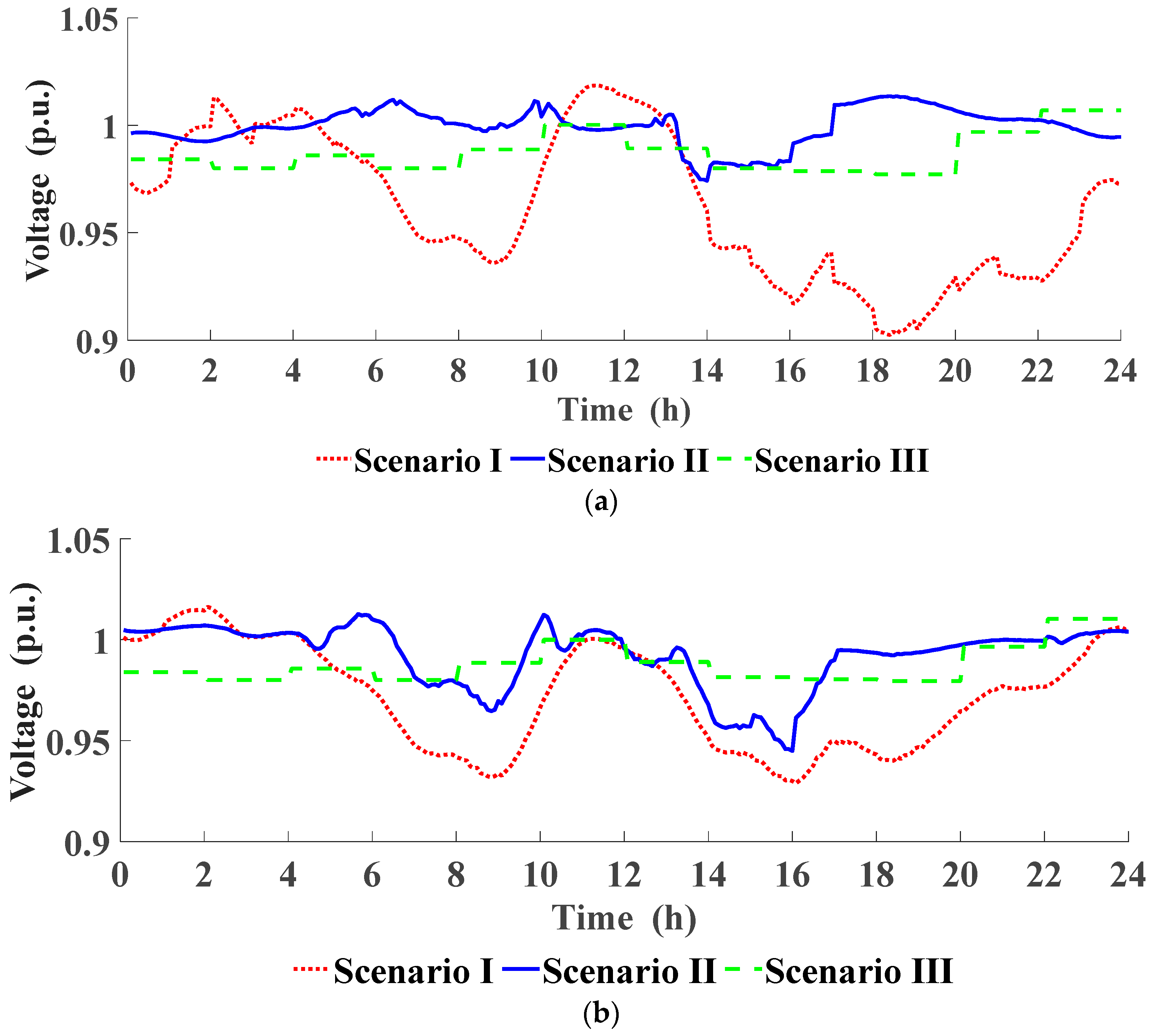
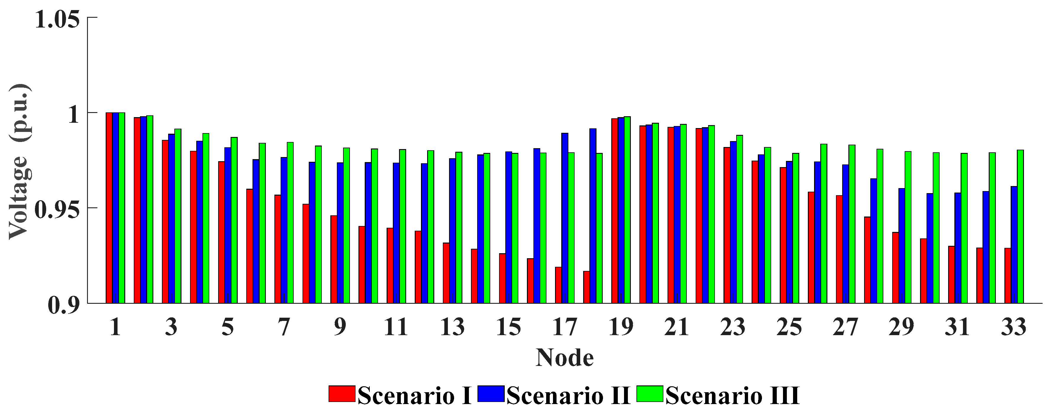
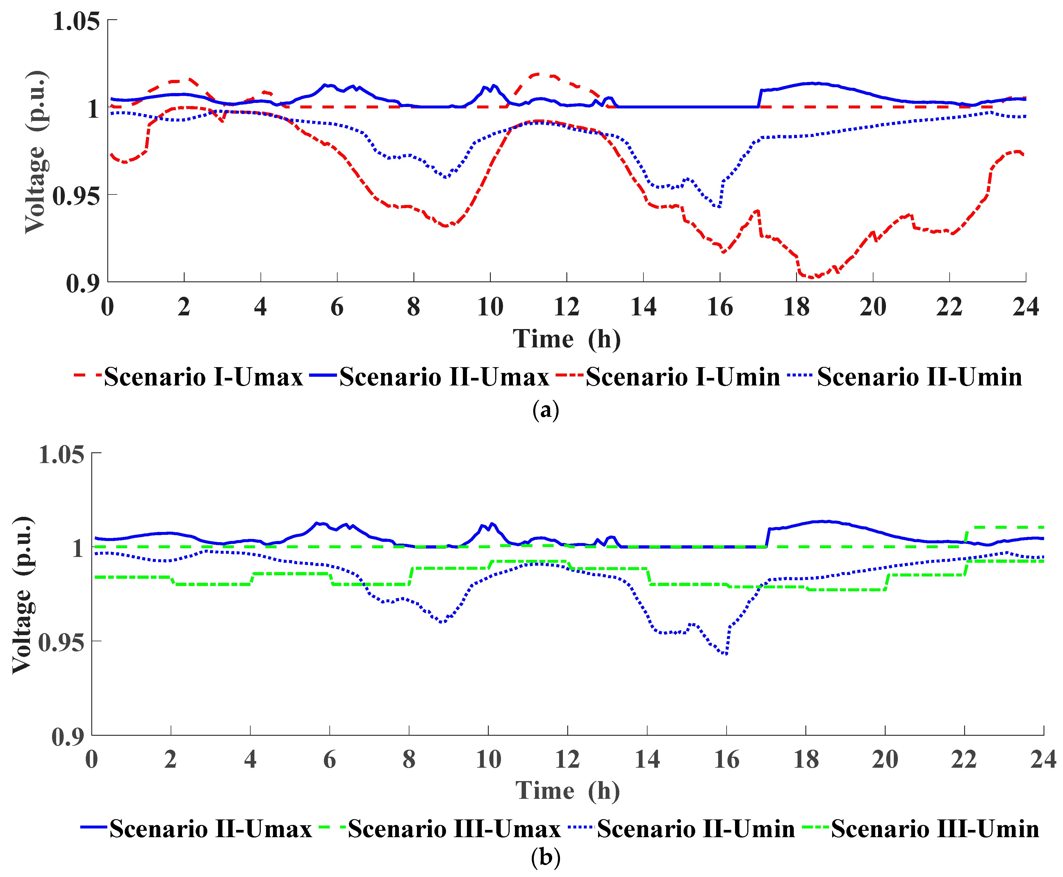
| Scenarios | Umax (p.u.) | Umin (p.u.) | VFI (p.u.) | Electricity Purchasing Cost (CNY) |
|---|---|---|---|---|
| I | 1.0189 | 0.9024 | 0.0205 | 4078.6 |
| II | 1.0136 | 0.9429 | 0.0077 | 3180.1 |
| III | 1.0103 | 0.9770 | 0.0086 | 2873.9 |
Disclaimer/Publisher’s Note: The statements, opinions and data contained in all publications are solely those of the individual author(s) and contributor(s) and not of MDPI and/or the editor(s). MDPI and/or the editor(s) disclaim responsibility for any injury to people or property resulting from any ideas, methods, instructions or products referred to in the content. |
© 2023 by the authors. Licensee MDPI, Basel, Switzerland. This article is an open access article distributed under the terms and conditions of the Creative Commons Attribution (CC BY) license (https://creativecommons.org/licenses/by/4.0/).
Share and Cite
Wang, G.; Qian, Z.; Feng, X.; Ren, H.; Zhou, W.; Wang, J.; Ji, H.; Li, P. Data-Driven Operation of Flexible Distribution Networks with Charging Loads. Processes 2023, 11, 1592. https://doi.org/10.3390/pr11061592
Wang G, Qian Z, Feng X, Ren H, Zhou W, Wang J, Ji H, Li P. Data-Driven Operation of Flexible Distribution Networks with Charging Loads. Processes. 2023; 11(6):1592. https://doi.org/10.3390/pr11061592
Chicago/Turabian StyleWang, Guorui, Zhenghao Qian, Xinyao Feng, Haowen Ren, Wang Zhou, Jinhe Wang, Haoran Ji, and Peng Li. 2023. "Data-Driven Operation of Flexible Distribution Networks with Charging Loads" Processes 11, no. 6: 1592. https://doi.org/10.3390/pr11061592