A Hybrid Model to Assess the Remaining Useful Life of Proton Exchange Membrane Fuel Cells

Abstract

Durability and remaining useful life (RUL) prediction techniques are ones of the key issues for proton exchange membrane fuel cell (FC) commercialization. Herein, the performance degradation of an FC is analyzed based on the whole lifetime experimental data (up to 6500 h). The voltage model with different patterns is developed based on the voltage data, which can be easily measured. The mechanism model is developed based on the evolution of degradation indices reflecting the degradation state. However, the former is sensitive to the local and periodic changes in the voltage curve, leading to a large prediction error, and the latter requires aging data from complex and high-cost characterization, limiting the practical applications. Therefore, a hybrid prediction model combining the voltage and mechanism model is proposed where the respective weight of each model is dynamically determined based on their local prediction errors. The results reveal that the maximum errors in RUL prediction are 9.72%, 3.90% and 2.01% for the voltage, mechanism and hybrid model, respectively, and the RUL prediction results of the hybrid model are close to actual RUL when those of the voltage model are far from the accuracy zone, indicating that the hybrid model provides credible RUL predictions with the highest accuracy.

1. Introduction

As one of the most promising devices for power generation, proton exchange membrane fuel cells (PEMFCs) are potential candidates in transportation, co-generation and military applications due to their high power density, environmental friendliness, light weight and abundant fuel sources [1]. However, before large-scale commercial applications, PEMFCs still need to overcome the challenges of high cost and poor durability. According to the statistics of the United States Department of Energy (DOE), the relevant indices for PEMFCs of current and target values are as follows, respectively: system cost (76 USD/kW vs. 30 USD/kW), peak energy efficiency (64% vs. 70%), power density (640 W/L vs. 850 W/L), specific power (860 W/kg vs. 900 W/kg) and durability in automotive drive cycle (4130 h vs. 8000 h) [2].

Performance degradation is one of the key reasons for the poor durability. Studying the aging mechanism and characteristics of the fuel cell (FC) is helpful to analyze the changes in performance and improve the remaining useful life (RUL). The aging study focuses on the proton exchange membrane (PEM), catalyst, gas diffusion layer (GDL) and bipolar plate (BP). The PEM is the main component of concern in FC, and the relevant studies include changes in PEM thickness [3], fluoride release rate (FRR), semi-empirical models based on the FRR [4] and the effect of hydrogen crossover [5,6,7]. The research on catalyst aging includes Pt dissolution/deposition mechanisms, corresponding models [8,9,10] and the modeling of the electrochemical active surface area (ECSA) reduction rate [11,12]. The aging of the GDL is mainly manifested by the changes in hydrophilicity and hydrophobicity, which are caused by the loss of the PTFE coating, the effect of thickness and porosity of the GDL [13,14,15]. Moreover, BP aging is mainly reflected in the deterioration of coating, which affects the contact resistance and, in turn, the performance of PEMFCs [16,17,18,19].

People expect to arrange maintenance timely by estimating RUL based on the previous operating status of an FC before the occurrence of trouble, which can extend the service life and reduce the cost. The prognostics methods of RUL are mainly divided into three categories: model-based methods, data-driven methods and hybrid methods [1].

The model-based methods are the most common and intuitive prognostic methods. The main principle is based on establishing some models related to PEMFCs, such as empirical models [20], semi-empirical models [21] and mechanism models [22], and then achieving the prognostics through filtering, statistics, machine learning and other technologies. The main advantage of the model-based method is that the changes in degradation index and state of PEMFCs can be observed with high accuracy. However, these model-based methods also suffer from the fact that the degradation mechanism is quite complex and some parameters of the models can only be determined based on the experimental data or expertise. The data-driven method typically utilizes machine learning algorithms [23], neural networks [24,25] and other algorithms to achieve the RUL estimation of PEMFCs. These methods are usually used when it is difficult to model the aging process. The main advantage is that these methods do not require an in-depth understanding of the degradation mechanism and just require a large set of aging data. However, these methods possess the black-box problem, i.e., key parameters and states of PEMFCs cannot be identified, compromising the effectiveness of maintenance measures.

Given the advantages and disadvantages of the model-driven and data-driven methods, different hybrid methods and strategies have been proposed to compensate for the shortcomings of model- and data-driven methods [26,27,28,29]. For instance, Hu et al. [27] have proposed a reconstructed lifetime-prediction model of an FC. Considering the temperature fluctuations and sensor errors, the voltage model was divided into three parts, and a degradation model with ECSA and resistance was added to the voltage model based on the degradation mechanism. The results demonstrated that the proposed model is credible and robust. Ma et al. [29] proposed a hybrid prediction method by combining the extended Kalman filter (EKF) with long- and short-term memory (LSTM) recurrent neural networks. In the training phase (TP), the EKF was used to obtain the prediction parameters and LSTM was trained with the FC output voltage. Overall, the RMSEs of voltage prediction were obtained as less than 0.0110, 0.0262 and 0.0317 using experimental data under static, quasi-dynamic and dynamic conditions, respectively.

In summary, hybrid methods for the lifetime prediction of PEMFCs are more concise and effective; however, there are still certain problems. In the published papers, the test time for FCs is far away from the actual lifetime, such as Silva’s 1200 h (2014) [30], Ma’s 1000 h (2017) [24] and Xie’s 1150 h (2022) [28]. Therefore, though these methods are feasible, the results may not be flawless, as the aging characteristics of some life periods of the FCs may not be presented. To propose a life-prediction model based on experimental data, the selection and processing of data are also critical. In practical applications, the output voltage or power is easy to be observed and commonly used as a health indicator (HI); however, a voltage model developed based on the measured voltage data is sensitive to the local or periodic changes in the voltage curve, leading to a large prediction error; another category of HIs, such as the ECSA, which directly shows the degradation degree, can only be periodically measured due to the complexity and cost. Therefore, it is difficult to achieve a simple and reliable RUL prediction of PEMFCs using aging data from either one of the categories alone.

In this study, the whole lifetime test data (>6500 h) of a fuel cell are analyzed. The voltage model is developed based on the measured voltage, where three models are used to compare the prediction results. The mechanism model is also developed based on the evolution of main degradation indicators, directly reflecting the degradation state of an FC. Furthermore, a hybrid prediction model based on the voltage and mechanism models is proposed to exploit the advantages of both models. A PF algorithm is used to eliminate random errors. The paper is structured as follows: Section 2 reports the lifetime test of a PEMFC; Section 3 introduces the PF algorithm; Section 4 presents the voltage model, mechanism model and hybrid model; Section 5 discusses the prognostic results of these models; and Section 6 summarizes the major results of this article.

2. Experimental Methods

The current data were obtained from the durability test of a single cell with a single-serpentine flow channel, as detailed elsewhere [22,31]. The MEA of the cell, prepared by WUT energy Co., Ltd., was selected with an active area of 25 cm²; Pt loading at anode and cathode was 0.1 and 0.4 mg/cm², respectively.

The cell was tested under steady-state conditions with a constant current density of 800 mA/cm². The operating temperature of the cell was 75 °C, the relative humidity of the anode and cathode were 70% and 50%, respectively, the stoichiometric ratios were both 2.0 and the back pressures were both 150 kPa. The test system included the GreenlightG20 test bench, an electrochemical workstation (Gamry Electrochemical Station, Interface5000E), an internal resistance tester (Applent, AT526) and a human–computer interaction interface, as shown in Figure 1.

The cell was shut down and purged every 100 h for characterization and performance measurements, including cyclic voltammetry (CV), linear sweep voltammetry (LSV), EIS and polarization curves (or current-voltage or I-V curves). The durability test lasted for 6562 h, but the time for intermediate purging, characterization and performance measurements was not included. Figure 2 shows the I-V, CV, LSV and EIS curves at some typical moments. Generally speaking, the I-V performance degrades with time, but at the end phase of the cell’s life, the degradation ration is much bigger than at the early time; the ECSA is decreased with time; the leakage current density is constant for a long time, but increases quickly at the end time, and the diffusion resistance increases with time. More details and quantity calculation can be found in [22].

The voltage evolution at a current density of 800 mA/cm² with time is shown in Figure 3. The time interval for each data point is 1 h. It can be seen that the voltage degradation during the whole lifetime is non-monotonic and non-linear. The FC performance slightly increased in the time interval of 0 to 5000 h, followed by a decrease at a slow rate for a long time and a rapid decline in the final stage. Across the entire lifetime of the FC, the contributions of the key factors (i.e., the ECSA, leakage current density, internal resistance and limiting current density) to voltage degradation significantly differed, resulting in the non-monotonic and non-linear characteristics of the aging performance [22]. Therefore, the fuel cell performance degradation curve cannot be fitted only with a simple linear model, as performed by some authors [32,33], due to the fact that the test time for their FCs is far away from the actual lifetime. The voltage suddenly increased after purging, characterization and performance measurements every 100 h due to the recovery of reversible degradation inside the FC. Though this behavior is beneficial to extend the FC’s lifetime, it makes the prediction of the voltage quite difficult.

3. Particle Filter

It can be seen that there are many data points, such as background noise, in Figure 3 which may be caused by different types of errors during aging testing. Meanwhile, resampling data per hour may cause some deviations from the real value. Hence, the relationship between output voltage and time is non-exact (with unknown coefficients), non-stationary and non-linear, as well as there may be an effect of the unknown noise distribution. These are the characteristics of a non-linear Bayesian tracking problem, and the particle filters solve this kind of problem [34].

The principle of particle filters is based on Monte Carlo methods that use sets of particles to represent probabilities. It can be applied to any type of the state-space equation. The tracking problem requires two equations, where the first one is the state equation, which needs to consider the change of system state [35]:

$$X_k=f(X_{k-1},W_k)$$

(1)

where k refers to the time index, X_k represents the state of the system at time k, f denotes the transition function from the state X_k-1 to the next state X_k and W_k refers to an independent identically distributed noise. The second is the observation equation [35]:

$$Z_k=h(X_k,V_k)$$

(2)

where Z_k refers to the result of observations, which is the voltage value of FC system, h denotes the observation function and V_k corresponds to the measurement noise, which refers to the measurement error of the G20 test station. The first stage is to split the initial state distribution $p\left(X_0\right)$, which is assumed known, into n particles. Then, the following three steps are repeated until the results are obtained.

(1)

Prediction: The n particles are propagated from time k − 1 to k by the state equation, and then gain a new system distribution.

$$p\left(X_k\left|Z_{1:k-1}\right.\right)={\displaystyle \int p\left(X_k\left|X_{k-1}\right.\right)p\left(X_{k-1}\left|Z_{k-1}\right.\right)d{X}_{k-1}}$$

(3)

(2)

Update: The likelihood function $p\left(Z_k\left|X_k\right.\right)$ of each particle is calculated based on the actual value, providing weight to each particle.

$$p\left(X_k\left|Z_{1:k}\right.\right)=\frac{p\left(Z_k\left|X_k\right.\right)p\left(X_k\left|Z_{1:k-1}\right.\right)}{p\left(Z_k\left|Z_{1:k-1}\right.\right)}$$

(4)

(3)

Re-sampling: A degeneracy phenomenon occurs with an increasing number of iterations, i.e., the number of particles with small weights tends to increase. Therefore, the particles with low weights are removed and particles with relatively large weights are copied via re-sampling. The recurrence formula of weight is:

$$\begin{gathered} W_k\left(X_k^{}\right)=\frac{p\left(Z_{1:k}\left|X_k\right.\right)p\left(X_k\right)}{q\left(X_k\left|Z_{1:k}\right.\right)}\propto \frac{p\left(\left.X_k\right|Z_{1:k}\right)}{q\left(X_k\left|Z_{1:k}\right.\right)} \\ =W_{k-1}^{}\frac{p\left(Z_k\left|X_k\right.\right)p\left(X_k\left|X_{k-1}\right.\right)}{q\left(X_k\left|X_{0:k-1},Z_{1:k}\right.\right)} \end{gathered}$$

(5)

4. Hybrid Prognostic Model

4.1. Prognostic Models for RUL

The FC voltage can be measured easily, and its change reflects the degradation of the FC itself. Therefore, it is often selected as an HI to determine the RUL of the FC.

4.1.1. Voltage Model

The linear model is simple, while the exponential and the logarithmic models are more accurate to track the rapid voltage decline in the final stage. Therefore, three voltage degradation models, including the linear model [32,33,36], the exponential model [35,36] and the logarithmic model, were chosen and compared to acquire the best suitable model.

(1)

The linear model:

$$y=a_1\cdot x+a_2$$

(6)

(2)

The exponential model:

$$y=b_1\cdot \exp (b_2\cdot x)+b_3\cdot x+b_4$$

(7)

(3)

The logarithmic model:

$$y=c_1\cdot \exp (c_2\cdot x)\ln (c_3\cdot x)+c_4$$

(8)

The state equations for the three models can be obtained using recursion:

(1)

The linear model:

$$X_k=a_1\cdot (t_k-t_{k-1})+X_{k-1}$$

(9)

(2)

The exponential model:

$$\begin{gathered} X_k=b_1\cdot (\exp (b_1\cdot (t_k-t_{k-1}))-1)\cdot \exp (b_2\cdot t_{k-1})+ \\ {b}_3\cdot (t_k-t_{k-1})+X_{k-1} \end{gathered}$$

(10)

(3)

The logarithmic model:

$$\begin{gathered} X_k=c_1\cdot \exp (c_1\cdot t_{k-1})\cdot (\exp (c_2\cdot (t_k-t_{k-1}))\ln (c_3\cdot t_k)- \\ \ln (c_3\cdot t_{k-1}))+X_{k-1} \end{gathered}$$

(11)

where X_k refers to the voltage value at time k, which is the result to be observed. Therefore, it is not necessary to construct the observation equation. These coefficients in the equations can be obtained by fitting the voltage curve.

4.1.2. Mechanism Model

The output voltage V_cell can be given as:

$$V_{cell}=E_{rev}-V_{act}-V_{ohm}-V_{con}$$

(12)

where E_rev refers to reversible voltage and V_act represents activation loss. The activation loss can be obtained by using the simplified Tafel equation:

$$V_{act}=\frac{\mathrm{RT}}{2\alpha \mathrm{F}}\ln \left(\frac{i+i_{loss}}{i_0}\right)$$

(13)

where α represents the charge transfer coefficient, i refers to the current density of FC, i_loss represents the leakage current density, which can be obtained from LSV, and i₀ denotes the exchange current density, which possesses the following function relationship with ECSA [12]:

$$i_0=i_0^{Pt}ECSA$$

(14)

During the durability test, the activity of the catalyst can be evaluated and the ECSA can be calculated from the CV. Therefore, we can gain a set of ECSA data, i.e., ECSA vs. time. Moreover, V_act can be calculated as follows:

$$V_{act}(t)=\frac{\mathrm{RT}}{2\alpha \mathrm{F}}\ln \left(\frac{i+i_{loss}(t)}{i_0^{Pt}ECSA\left(t\right)}\right)$$

(15)

The final V_act expression can be given as:

$$V_{act}(t)=\frac{\mathrm{RT}}{2\alpha \mathrm{F}}\left[\ln \left(\frac{i+i_{loss}(t)}{i_0^{Pt}ECSA\left(t_0\right)}\right)-\ln \left(\frac{ECSA(t)}{ECSA\left(t_0\right)}\right)\right]$$

(16)

The ohmic loss V_ohm can be given by Ohm’s law:

$$V_{ohm}(t)=i\cdot \left(R_{ele}+R_{ion}+R_{contact}\right)$$

(17)

where R_ele refers to electronic resistance, R_ion represents ionic resistance and R_contact denotes contact resistance. The sum of these can be determined using high frequency resistance (HFR) experimentally. HFR can be recorded with the G20 test station. Therefore, the ohmic loss V_ohm can be given as:

$$V_{ohm}(t)=i\cdot R_{HRF}(t)$$

(18)

The diffusion loss V_con can be evaluated as [12]:

$$V_{con}=\overline{\omega }\mathrm{T}i\cdot \ln \left(\frac{i_L}{i_L-i}\right)$$

(19)

where $\overline{\omega }$ refers to an empirical constant. i_L represents the limiting current density that can be obtained by fitting the polarization curve. Moreover, V_con can be given as:

$$V_{con}(t)=\overline{\omega }\mathrm{T}i\cdot \ln \left(\frac{i_L(t)}{i_L(t)-i}\right)$$

(20)

It can be seen that the voltage output is divided into four parts. The reversible voltage is affected by the temperature and partial pressure of hydrogen and oxygen, but there is only a little variation in temperature and partial pressure during the durability test. Hence, the effect on reversible voltage can be neglected. Therefore, the variation in voltage depends on activation loss, ohmic loss and diffusion loss. The degradation indices that affect the lifetime of the FC include leakage current density, exchange current density, resistance and limiting current density [22]. The leakage current density is mainly related to gas crossover and electronic short-circuit. The exchange current density reflects the electrochemical reaction rate and is connected with the performance of the catalyst layer (CL), whereas the change in ECSA is used to evaluate the performance of the CL. The resistance of the FC that can be replaced by HFR is mainly affected by the resistance of membrane and bipolar plate. The limiting current is proportional to the diffusion coefficient; thus, the change in limiting current reflects the aging state of the GDL.

Based on the above discussion, the functional relationships of these indices and time can be obtained by choosing suitable models to fit the data. Then, the state equations of these indices can be achieved via recursion. By combining Equations (12)–(20), the state equation and observation equation of the mechanism model are as follows:

$$\left[\begin{array}{c}{i}_{loss}(k+1)\\ ECSA(k+1)\\ R_{HFR}(k+1)\\ i_L(k+1)\end{array}\right]=\left[\begin{array}{c}{i}_{loss}(k)\\ ECSA(k)\\ R_{HFR}(k)\\ i_L(k)\end{array}\right]+W_k$$

(21)

$$\begin{gathered} V_{\mathrm{cell}}(k)=E_{rev}-\frac{\mathrm{RT}}{2\alpha \mathrm{F}}\left[\ln \left(\frac{i+i_{loss}(k)}{i_0^{Pt}ECSA\left(t_0\right)}\right)-\ln \left(\frac{ECSA(k)}{ECSA\left(t_0\right)}\right)\right]- \\ i\cdot R_{HFR}(k)-\overline{\omega }\mathrm{T}i\cdot \ln \left(\frac{i_L(k)}{i_L(k)-i}\right)+V_k \end{gathered}$$

(22)

4.2. Hybrid Diagnostic Approach

As mentioned above, the voltage model and mechanism model can be used to make predictions of RUL, marked as RUL₁ and RUL₂, respectively. The advantages and disadvantages of the two models are as follows:

• The advantages of the voltage model are as follows—the voltage as a degradation index is easy to be measured; the degradation trend can be observed directly. While its disadvantages are—the fuel cell can be observed being degraded, but the degradation mechanism cannot be understood directly; the predicted RUL is sensitive to the local variation of the measured data, which many affect the prediction accuracy.
• For the mechanism model, though aging indices reflect the internal aging state of the FC, the data used by this model are obtained from the characterization and performance test after shutdown, which are complex and high-cost; therefore, related data are not abundant, with poor practicality.

Hence, to take advantage of the voltage and mechanism models, the hybrid diagnostic approach is proposed and shown in Figure 4. The hybrid model can be given as:

$$RU{L}_t^{*}={\displaystyle \sum }_{n=1}^2{w}_{t,n}\cdot \left(RU{L}_{t,n}-B_{t,n}\right)$$

(23)

where $RU{L}_t^{*}$ represents the hybrid prognostic RUL at time t, RUL_t,n (n = 1, 2) refers to the prognostic RUL of the voltage and mechanism models, respectively, and w_t denotes the weighing factor. The weights should be changed according to their local prediction accuracy at different time steps dynamically. It is anti-correlated with the error. Moreover, the weighting factor can be calculated by the inverse of error, i.e.,

$$w_t=\frac{1/Er{r}_{t,1}}{\left(1/Er{r}_{t,1}+1/Er{r}_{t,2}\right)}$$

(24)

where Err_t,n refers to the prediction absolute error of both models at time t. It can be defined at time t for the n^th model as below:

$$Er{r}_{t,n}=\frac{1}{\mathrm{m}}{\displaystyle \sum _{k=1}^{\mathrm{m}}\left|RU{L}_t^{real}-RU{L}_{t,n}^{prediction}\right|}$$

(25)

where $RU{L}_t^{real}$ refers to the true RUL and $RU{L}_t^{prediction}$ represents the predicted RUL of the k^th curve predicted by the n^th model at time step t, and m denotes the number of nearest trajectories. Considering the insufficient available observations at shorter TPs, the model provides predictions with large variations. By introducing the average variation of the model (B_t,n), used as an offset, the effect can be effectively reduced [37]:

$$B_{t,n}=\frac{1}{\mathrm{m}}{\displaystyle \sum _{k=1}^{\mathrm{m}}\left(RU{L}_t^{real}-RU{L}_{t,n}^{prediction}\right)}$$

(26)

5. Results and Discussion

5.1. Degradation Prediction Based on the Voltage Model

5.1.1. Voltage Aging Prediction

According to Equations (6)–(8), the initial values of coefficients were obtained by fitting the voltage curves during the training phase. Both the linear and logarithmic models can capture the voltage drop trend when the TP is more than 4500 h, while the exponential model can predict it when the TP is more than 5300 h. Thus, TP = 5300–6500 h was uniformly chosen to be compared. The number of particles of three model coefficient filters was 3000. For each set of the model coefficients, the voltage was calculated with 100 times and the means of the results were used as the outputs. Figure 5 presents the voltage prediction results of three models at different TPs.

Figure 5a shows the voltage prediction of three models with the TP at 5249 h. It can be seen that the linear model can only reflect the declining trend of the voltage, but it fails to predict the rapid decreasing trend after 5900 h. Herein, the rapid decreasing trend in the later stage can be well-predicted by both exponential and logarithmic models, and the predicted data match well with the measured data. However, the recovery phenomenon has not been captured by these models. Therefore, compared with both the logarithmic and exponential models, the linear model is inaccurate.

Figure 5b,c show the voltage prediction of exponential and logarithmic models at different TPs, respectively. Herein, the time increase step was 100 h for each TP, starting from 5300 h to 6500 h. It can be seen that the voltage model is sensitive to local and periodic changes in the voltage curves. For instance, as shown in Figure 5b for a TP of 5300 h, the local trend at 5300 h is flat, which results in a predicted RUL of more than 8000 h. On the other hand, in the case of TP = 5600 h, the local trend at 5600 h is decreasing, which results in a predicted RUL of around 5700 h. In the case of the logarithmic model (Figure 5c), it can be seen that the predicted RULs are also affected by TPs (or by the local/periodic changes in voltage curves). However, the influence of different TPs is far lower than in Figure 5b. Herein, large differences among voltage prediction curves for different TPs show that a shorter TP corresponds to a larger prediction error.

To compare the prediction accuracy of three models for voltage degradation, the root mean square error (RMSE) and mean absolute percent error (MAPE) were introduced to evaluate the voltage prediction. The calculation formulas are as follows:

$$\mathrm{RMSE}=\sqrt{\frac{1}{m}{\displaystyle \sum }_{i=1}^m{\left({\widehat{y}}_i-y_i\right)}^2}$$

(27)

$$\mathrm{MAPE}=\frac{1}{m}{\displaystyle \sum _{i=1}^m\frac{\left|{\widehat{y}}_i-y_i\right|}{\left|y_i\right|}}\times 100$$

(28)

RMSE and MAPE of three models at different TPs are listed in

Table 1. The RMSE and MAPE of three models.

	Linear Model		Exponential Model		Logarithmic Model
TP	RMSE	MAPE	RMSE	MAPE	RMSE	MAPE
5300	0.01436	1.441	0.01431	1.446	0.01274	1.472
5400	0.01468	1.467	0.01147	1.239	0.01238	1.414
5500	0.01454	1.455	0.01622	1.429	0.01097	1.165
5600	0.01399	1.431	0.01871	1.582	0.01089	1.158
5700	0.01422	1.430	0.01951	1.634	0.01096	1.157
5800	0.01399	1.414	0.01628	1.470	0.01129	1.220
5900	0.01388	1.428	0.01422	1.561	0.01083	1.157
6000	0.01375	1.427	0.01112	1.159	0.01084	1.152
6100	0.01370	1.445	0.01412	1.343	0.01078	1.152
6200	0.01360	1.442	0.01133	1.247	0.01104	1.184
6300	0.01342	1.430	0.01115	1.176	0.01097	1.172
6400	0.01377	1.520	0.01614	1.491	0.01133	1.247
6500	0.01336	1.446	0.01094	1.168	0.01097	1.166

, whereas stacked RMSE and MAPE plots are drawn in Figure 5d,e. It can be seen that the RMSE of the logarithmic model keeps the lowest value except for the TP at 5400 h and the MAPE keeps the lowest value after 5500 h. Both the MAPE and RMSE tend to gradually decrease with the increase in learning time. Though the exponential model exhibits a similar decrease, the stacked values are larger than the logarithmic model. Moreover, the RMSE of the linear model remains constant, but the RMSE value of the linear model is higher than that of the logarithmic model, and the stacked MAPE is the highest among three models. Thus, it can be seen that the logarithmic model renders the highest accuracy.

5.1.2. RUL Estimations

The RUL of fuel cells can be determined based on the failure threshold of the output voltage value. The actual end-of-life (EOL) threshold for the PEMFC is a 10% loss of initial voltage defined by the DOE [2]. Therefore, a 10% decrease in voltage is used as the EOL threshold. RUL is the time interval between the time when the prediction begins and when the prediction voltage first reaches the EOL threshold. Due to the poor results of the linear model, RUL predictions of the linear model are not discussed further. To assess the RUL prediction quality of the exponential and logarithmic models, α metric [38] and satisfactory horizon (SH) [2] were applied as evaluation criteria.

(1)

α metric is the allowable error bound around the actual RUL, which is taken as α = ±5% in this paper, meeting the prediction requirements of industrial applications [38]. If the prediction point stands in the interval of the accuracy zone, it is considered that the prediction result meets the accuracy requirements, which is an on-time prediction. There are two other cases: early predictions and late predictions. Early prediction means that the predicted RUL is smaller than the actual RUL and the point falls below the accuracy zone. Late prediction means that the predicted RUL is greater than the actual RUL and the point falls above the accuracy zone. The late prediction indicates that the prediction exceeds the actual value, which cannot warn users in time to make a decision for maintenance or adjust operating conditions. Therefore, on-time prediction and early prediction are more meaningful and desirable [2]. The number of prediction points in each region is denoted by N.

(2)

SH is defined as a duration when the prediction in the interval of allowable error range is around the actual RUL [2]. Herein, the SH can evaluate the prediction ability of the model, and a high SH value corresponds to a better prediction quality.

Moreover, the RUL predictions of these models are calculated at different TPs, where the time step for each TP is 100 h, starting from 5300 h to 6500 h. Figure 6a,b shows RUL predictions for 100 calculations of the exponential and logarithmic models. The red mark in the middle of the box signifies the median and the red dot shows the average value. It can be seen that the predicted value of the exponential model differs significantly from the actual RUL value before 5800 h and is always in the interval of the accuracy zone after 5800 h, where the predicted value of the logarithmic model enters the interval of the accuracy zone after 5500 h. Therefore, the SH value of exponential model is 700 h, which is smaller than the corresponding value of the logarithmic model. It means that the RUL prediction of the logarithmic model is more reliable than that of the exponential model.

Table 2. The prediction performance with α-metrics.

N	Exponential	Logarithmic
Early prediction	3	0
On-time prediction	8	11
Late prediction	2	2
sum	13	13

shows the number of prediction points falling in three regions for two models. It is clear that the logarithmic model has more points falling in the interval of the accuracy zone than the exponential model.

After 5900 h, RUL predictions of the exponential and logarithmic models are quite similar in the interval of the accuracy zone. It can be also readily observed that the logarithmic model exhibits a shorter box, implying that it is more stable than the exponential model.

Table 3. Error dispersion between the 25th and 75th percentiles of the RUL prediction.

	Exponential	Logarithmic
Minimum range	20	30
Average range	106.5	56
Maximum range	252.5	122.5

shows the error dispersion of both models between the 25th and 75th percentiles. It can be seen that the average dispersion of the exponential model is 106.5 h, while the corresponding value for the logarithmic model is 56 h. Though the RUL prediction of the exponential model after 5900 h is closer to the true value compared with that of the logarithmic model, the dispersion over 100 h cannot be neglected. Thus, only the logarithmic model and relevant results are used in the following section.

5.2. Degradation Prediction Based on the Mechanism Model

5.2.1. Voltage Aging Prediction

The degradation indices can be predicted based on the PF algorithm, reflecting the degradation state of the inner components or materials of FCs. The different degradation processes during the whole lifetime can be reflected by the variation of the four degradation indices. The calculation results of this model at some important moments are listed in

Table 4. Calculation results of the mechanism model.

Time	Characteristic	iloss /A cm−2	ECSA /m2 g−1	HFR /mOhm cm−2	ilim /A cm−2	Output Voltage /V
T = 0 h	Value	0.00304	21.952	1.851	2.248	0.718
	Voltage drop/V	0.00011	0.401	0.033	0.036
T = 2000 h	Value	0.00332	9.837	1.757	2.695	0.699
	Voltage drop/V	0.00012	0.421	0.0351	0.0333
	Relative change ratio	0.092	−0.552	−0.051	0.199
T = 5000 h	Value	0.00449	12.928	1.716	2.643	0.708
	Voltage drop/V	0.00017	0.412	0.0343	0.0341
	Relative change ratio	0.477	−0.411	−0.073	0.176
T = 6562 h	Value	0.08100	6.352	1.741	1.886	0.663
	Voltage drop/V	0.00289	0.433	0.0348	0.0544
	Relative change ratio	25.645	−0.711	−0.059	−0.161

. It can be seen that the ECSA was reduced a lot at 2000 h and the output voltage decreased correspondingly to 0.699V, which has the same trend as shown in Figure 3. Then, i_loss was generally stable at 5000 h. The HFR was reduced a bit compared with the initial values, and the i_lim had a larger value at 5000 h than at 0 h; within about 0–5000 h, according to our calculation, the contributions of i_lim and HFR evolution to voltage loss were negative. Thus, the voltage was generally stable before 5000 h. It can be also found that at 6562 h the relative change ratios of i_loss and ECSA changed more than two other indices, and activation loss caused by the decrease in i_loss and ECSA mainly contributed to the output voltage drop. It can be concluded that the degradation rates of the membrane and CL are higher than those of the GDL.

The voltage prediction results for the FC with different TPs, ranging from 3000 h to 6500 h with a step size of 500 h, are shown in Figure 7a. It can be seen that the mechanism model can predict the decreasing trend of voltage in a shorter learning time compared with the voltage model, and the predicted voltage values exhibit a higher decreasing rate than those of the measured voltage. Additionally, the rate of decrease increases with an increase in TP. Therefore, the mechanism model underestimates the RUL.

To confirm the prediction accuracy of the mechanism model, the RMSE and MAPE are listed in

Table 5. RMSE and MAPE of the mechanism model.

TP	RMSE	MAPE	TP	RMSE	MAPE
5300	0.0232	2.349	6000	0.01760	2.021
5400	0.02248	2.313	6100	0.02141	2.394
5500	0.02189	2.372	6200	0.02349	2.524
5600	0.03144	2.492	6300	0.02210	2.410
5700	0.02636	2.562	6400	0.02163	2.428
5800	0.02257	2.318	6500	0.02499	2.493
5900	0.02496	2.371

, and the stacked RMSE and MAPE plots, with TP = 5300–6500 h, are presented in Figure 7b,c. It can be seen that both the RMSE and MAPE of the mechanism model are larger than those of the voltage model. This is caused by the fact that the prediction voltage of the mechanism model is calculated with the four degradation indices, which contain some errors obtained from three factors: calculation error from the mechanism model, fitting error between the observed and estimated value of the four degradation indices and human errors from the model simplification.

5.2.2. RUL Estimation

Compared with the voltage model, RUL predictions of the mechanism model are calculated from 5300 h to 6500 h with an interval of 100 h. Figure 8 shows the RUL prediction distribution of the mechanism model.

Though the prediction points are in the interval of allowable error range, it can be seen that the mechanism model underestimates the RUL. This indicates that the mechanism model is reliable and gives on-time predictions with different TPs. The box plot also shows that the distribution becomes more concentrated with the increase in TP. In fact, the average error dispersion of the mechanism model is 257.1 h in the 25th and 75th percentiles against the voltage model of 56 h in

Table 6. Error dispersion between the 25th and 75th percentiles of the RUL prediction.

	Voltage	Mechanism
Minimum range	30	200
Average range	56	257.1
Maximum range	122.5	300

. It means that the mechanism model underestimates the RUL, while the dispersion of prediction results is relatively large.

5.3. Comparison with the Hybrid Model

In practical applications, it is expected to obtain a great number of aging trajectories, i.e., aging data, to predict the RUL of the same fuel cell group. Herein, the prediction errors are obtained based on the 10 selected nearest curves (m = 10 in Equation (25)) from the 100 curves calculated previously. Figure 9a shows the distribution of average error of two models at different TPs. It can be seen that the voltage model has a relatively large error at first and it decreases with increasing TP in the later stages. Hence, the overall error of the mechanism model is smaller than that of the voltage model, which increases during the last stage.

Figure 9b shows the dynamic assignment of the weighting factors of each model according to the prediction errors. The weights of the mechanism model are larger than those of the voltage model before 5500 h and decrease after, which are smaller than the corresponding values of the voltage model at some points but conversely at other points, indicating that the prediction quality of the voltage model rapidly improves with increasing training time.

Figure 10a compares the RUL predictions of three models. It can be seen that the prediction results of the hybrid model can almost totally enter the interval, except for one point at a TP of 4800 h, and the SH of the hybrid model is 1600 h. It is worth emphasizing that the RUL prediction results of the hybrid model are still close to the actual RUL when the RUL of the voltage method is far from the 2α interval before 5500 h. The RUL prediction errors for three models, ranging from 4500 h to 6500 h with an interval of 100 h, is shown in Figure 10b. It can be seen that the prediction error of the hybrid model is the minimum for almost all training phases. Overall, the results reveal that when the TP is more than 4500 h, the errors in the RUL prediction are less than 9.72%, 3.90% and 2.01% for the voltage, mechanism and hybrid model, respectively, indicating that the hybrid model provides credible RUL predictions with the highest accuracy.

6. Conclusions

In summary, the evolution characteristics of the performance degradation of the fuel cell are analyzed based on the whole lifetime data (up to 6500 h). The RUL prediction models of the fuel cell and prediction accuracy are studied in detail. The main conclusions can be drawn as follows:

(1)

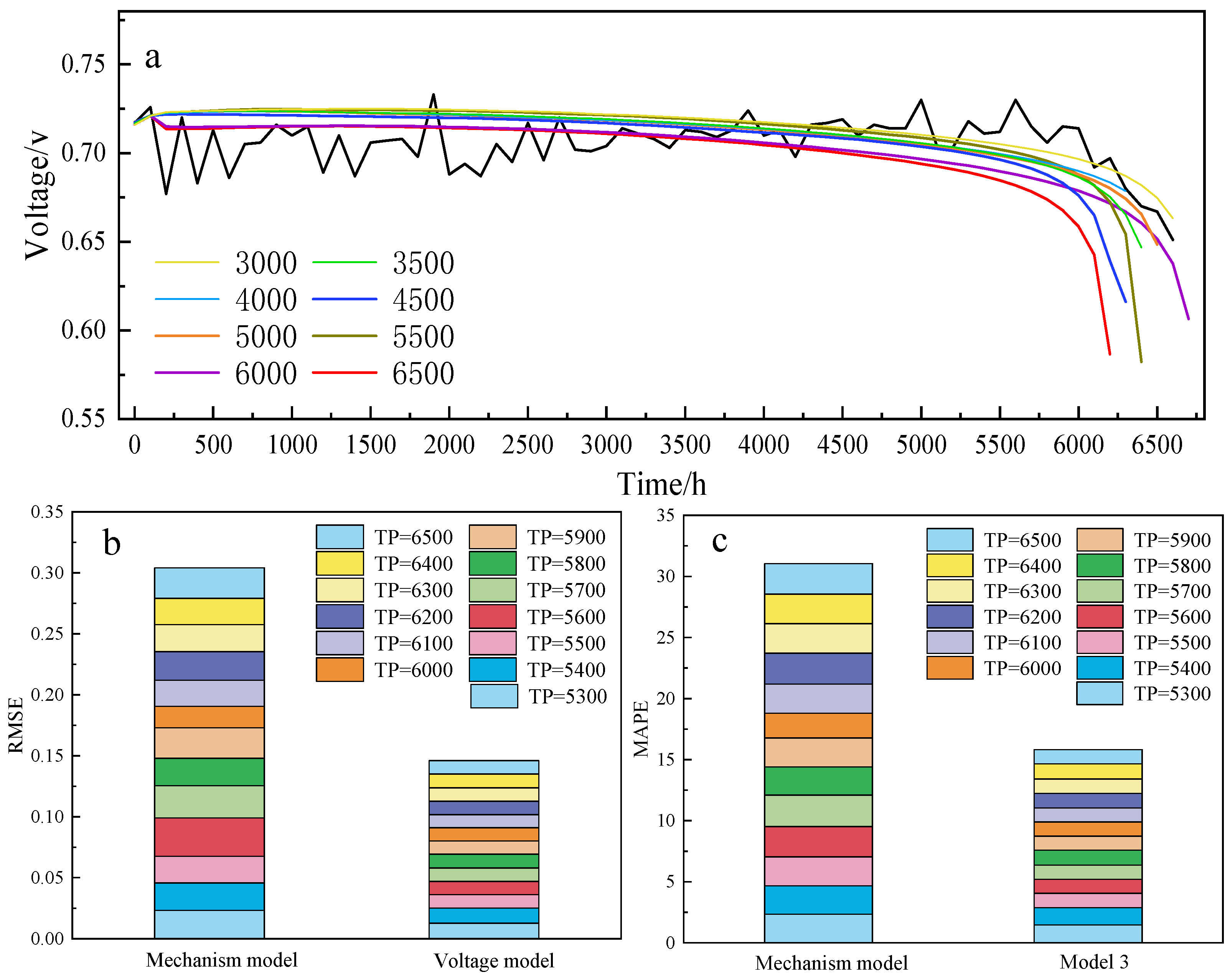
The overall trend of the performance degradation curve of the FC varies during different periods of the whole lifetime, which slightly increases from 0 to 5000 h and decreases at a small rate for a long time, followed by a rapid decline at the end of life. Therefore, the fuel cell performance degradation curve exhibits non-monotonic and non-linear characteristics which cannot be fitted only with a simple linear model.

(2)

The voltage model was developed based on the voltage data, which can be measured easily, and the prediction accuracy of linear, exponential and logarithmic models is compared. The results reveal that the logarithm model can assess the characteristics of rapid voltage decrease with a shorter TP than other models, and the stacked RMSE and MAPE are the lowest. The RUL prediction value is more stable, with an average dispersion of 56 h. The prediction performance of the voltage model improves with increasing training time. However, this model is sensitive to local and periodic changes in the voltage curve, which leads to a relatively large prediction error with a short TP.

(3)

The mechanism model was developed based on the evolution characteristics of degradation indices, which can reflect the degradation of FCs. It is found that the activation loss caused by the decrease in i_loss and ECSA contributes most to the output voltage drop, and the degradation rate of the membrane and CL is higher than that of the GDL. The mechanism model is reliable and underestimates RUL, whereas the dispersion of prediction results is relatively large and it requires aging data from complex and high-cost characterization and performance tests, limiting practical applications.

(4)

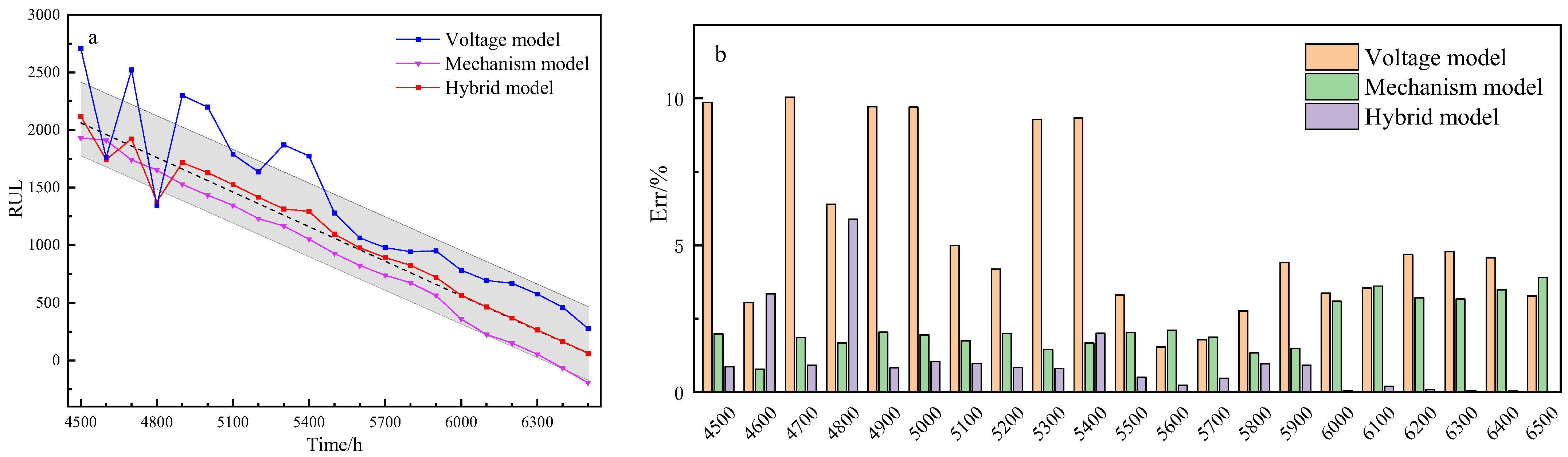
The hybrid model combining the voltage and mechanism models is proposed to utilize the advantages of each model. The results reveal that when the TP is more than 4500 h, the errors of RUL prediction are less than 9.72%, 3.90% and 2.01% for the voltage, mechanism and hybrid model, respectively. The RUL prediction results of the hybrid model are close to the actual RUL when the prediction results of the voltage method are far from the accuracy zone. Hence, the proposed hybrid model provides credible RUL predictions with the highest accuracy.

These results confirm that the hybrid model is significant for predicting the RUL of PEMFCs. For a group of PEMFCs composed with the same materials and the same structural components/assemblies, the hybrid model combines aging data from different, but related, sources, which can effectively improve the accuracy of RUL predictions and give out the degradation causes.

References

1. Liu, H.; Chen, J.; Hissel, D.; Lu, J.; Hou, M.; Shao, Z. Prognostics Methods and Degradation Indexes of Proton Exchange Membrane Fuel Cells: A Review. Renew. Sustain. Energy Rev. 2020, 123, 109721. [Google Scholar] [CrossRef]
2. Hua, Z.; Zheng, Z.; Pahon, E.; Péra, M.-C.; Gao, F. A Review on Lifetime Prediction of Proton Exchange Membrane Fuel Cells System. J. Power Sources 2022, 529, 231256. [Google Scholar] [CrossRef]
3. Zhao, M.; Shi, W.; Wu, B.; Liu, W.; Liu, J.; Xing, D.; Yao, Y.; Hou, Z.; Ming, P.; Zou, Z. Influence of Membrane Thickness on Membrane Degradation and Platinum Agglomeration under Long-Term Open Circuit Voltage Conditions. Electrochim. Acta 2015, 153, 254–262. [Google Scholar] [CrossRef]
4. Chandesris, M.; Vincent, R.; Guetaz, L.; Roch, J.-S.; Thoby, D.; Quinaud, M. Membrane Degradation in PEM Fuel Cells: From Experimental Results to Semi-Empirical Degradation Laws. Int. J. Hydrogen Energy 2017, 42, 8139–8149. [Google Scholar] [CrossRef]
5. Inaba, M.; Kinumoto, T.; Kiriake, M.; Umebayashi, R.; Tasaka, A.; Ogumi, Z. Gas Crossover and Membrane Degradation in Polymer Electrolyte Fuel Cells. Electrochim. Acta 2006, 51, 5746–5753. [Google Scholar] [CrossRef]
6. Truc, N.T.; Ito, S.; Fushinobu, K. Numerical and Experimental Investigation on the Reactant Gas Crossover in a PEM Fuel Cell. Int. J. Heat Mass Transf. 2018, 127, 447–456. [Google Scholar] [CrossRef]
7. Tang, Q.; Li, B.; Yang, D.; Ming, P.; Zhang, C.; Wang, Y. Review of Hydrogen Crossover through the Polymer Electrolyte Membrane. Int. J. Hydrogen Energy 2021, 46, 22040–22061. [Google Scholar] [CrossRef]
8. Bi, W.; Fuller, T.F. Modeling of PEM Fuel Cell Pt/C Catalyst Degradation. J. Power Sources 2008, 178, 188–196. [Google Scholar] [CrossRef]
9. Robin, C.; Gérard, M.; Quinaud, M.; d’Arbigny, J.; Bultel, Y. Proton Exchange Membrane Fuel Cell Model for Aging Predictions: Simulated Equivalent Active Surface Area Loss and Comparisons with Durability Tests. J. Power Sources 2016, 326, 417–427. [Google Scholar] [CrossRef]
10. Ren, P.; Pei, P.; Li, Y.; Wu, Z.; Chen, D.; Huang, S. Degradation Mechanisms of Proton Exchange Membrane Fuel Cell under Typical Automotive Operating Conditions. Prog. Energy Combust. Sci. 2020, 80, 100859. [Google Scholar] [CrossRef]
11. Reid, O.; Saleh, F.S.; Easton, E.B. Determining Electrochemically Active Surface Area in PEM Fuel Cell Electrodes with Electrochemical Impedance Spectroscopy and Its Application to Catalyst Durability. Electrochim. Acta 2013, 114, 278–284. [Google Scholar] [CrossRef]
12. Polverino, P.; Pianese, C. Model-Based Prognostic Algorithm for Online RUL Estimation of PEMFCs. In Proceedings of the 2016 3rd Conference on Control and Fault-Tolerant Systems (SysTol), Barcelona, Spain, 7–9 September 2016; IEEE: Barcelona, Spain, 2016; pp. 599–604. [Google Scholar]
13. Baik, K.D.; Kim, S.I.; Hong, B.K.; Han, K.; Kim, M.S. Effects of Gas Diffusion Layer Structure on the Open Circuit Voltage and Hydrogen Crossover of Polymer Electrolyte Membrane Fuel Cells. Int. J. Hydrogen Energy 2011, 36, 9916–9925. [Google Scholar] [CrossRef]
14. Lapicque, F.; Belhadj, M.; Bonnet, C.; Pauchet, J.; Thomas, Y. A Critical Review on Gas Diffusion Micro and Macroporous Layers Degradations for Improved Membrane Fuel Cell Durability. J. Power Sources 2016, 336, 40–53. [Google Scholar] [CrossRef]
15. Pan, Y.; Wang, H.; Brandon, N.P. Gas Diffusion Layer Degradation in Proton Exchange Membrane Fuel Cells: Mechanisms, Characterization Techniques and Modelling Approaches. J. Power Sources 2021, 513, 230560. [Google Scholar] [CrossRef]
16. Zhang, L.; Liu, Y.; Song, H.; Wang, S.; Zhou, Y.; Hu, S.J. Estimation of Contact Resistance in Proton Exchange Membrane Fuel Cells. J. Power Sources 2006, 162, 1165–1171. [Google Scholar] [CrossRef]
17. Lin, C.-H.; Tsai, S.-Y. An Investigation of Coated Aluminium Bipolar Plates for PEMFC. Appl. Energy 2012, 100, 87–92. [Google Scholar] [CrossRef]
18. Orsi, A.; Kongstein, O.E.; Hamilton, P.J.; Oedegaard, A.; Svenum, I.H.; Cooke, K. An Investigation of the Typical Corrosion Parameters Used to Test Polymer Electrolyte Fuel Cell Bipolar Plate Coatings, with Titanium Nitride Coated Stainless Steel as a Case Study. J. Power Sources 2015, 285, 530–537. [Google Scholar] [CrossRef]
19. Yang, L.X.; Liu, R.J.; Wang, Y.; Liu, H.J.; Zeng, C.L.; Fu, C. Corrosion and Interfacial Contact Resistance of Nanocrystalline β-Nb2N Coating on 430 FSS Bipolar Plates in the Simulated PEMFC Anode Environment. Int. J. Hydrogen Energy 2021, 46, 32206–32214. [Google Scholar] [CrossRef]
20. Jouin, M.; Gouriveau, R.; Hissel, D.; Péra, M.-C.; Zerhouni, N. Prognostics of PEM Fuel Cell in a Particle Filtering Framework. Int. J. Hydrogen Energy 2014, 39, 481–494. [Google Scholar] [CrossRef]
21. Lechartier, E.; Laffly, E.; Péra, M.-C.; Gouriveau, R.; Hissel, D.; Zerhouni, N. Proton Exchange Membrane Fuel Cell Behavioral Model Suitable for Prognostics. Int. J. Hydrogen Energy 2015, 40, 8384–8397. [Google Scholar] [CrossRef]
22. Chen, H.; Zhan, Z.; Jiang, P.; Sun, Y.; Liao, L.; Wan, X.; Du, Q.; Chen, X.; Song, H.; Zhu, R.; et al. Whole Life Cycle Performance Degradation Test and RUL Prediction Research of Fuel Cell MEA. Appl. Energy 2022, 310, 118556. [Google Scholar] [CrossRef]
23. Wu, Y.; Breaz, E.; Gao, F.; Paire, D.; Miraoui, A. Nonlinear Performance Degradation Prediction of Proton Exchange Membrane Fuel Cells Using Relevance Vector Machine. IEEE Trans. Energy Convers. 2016, 31, 1570–1582. [Google Scholar] [CrossRef]
24. Ma, R.; Yang, T.; Breaz, E.; Li, Z.; Briois, P.; Gao, F. Data-Driven Proton Exchange Membrane Fuel Cell Degradation Predication through Deep Learning Method. Appl. Energy 2018, 231, 102–115. [Google Scholar] [CrossRef]
25. Hua, Z.; Zheng, Z.; Pahon, E.; Péra, M.-C.; Gao, F. Remaining Useful Life Prediction of PEMFC Systems under Dynamic Operating Conditions. Energy Convers. Manag. 2021, 231, 113825. [Google Scholar] [CrossRef]
26. Sankavaram, C.; Pattipati, B.; Kodali, A.; Pattipati, K.; Azam, M.; Kumar, S.; Pecht, M. Model-Based and Data-Driven Prognosis of Automotive and Electronic Systems. In Proceedings of the 2009 IEEE International Conference on Automation Science and Engineering, Bangalore, India, 22–25 August 2009; IEEE: Bangalore, India, 2009; pp. 96–101. [Google Scholar]
27. Hu, Z.; Xu, L.; Li, J.; Ouyang, M.; Song, Z.; Huang, H. A Reconstructed Fuel Cell Life-Prediction Model for a Fuel Cell Hybrid City Bus. Energy Convers. Manag. 2018, 156, 723–732. [Google Scholar] [CrossRef]
28. Xie, Y.; Zou, J.; Li, Z.; Gao, F.; Peng, C. A Novel Deep Belief Network and Extreme Learning Machine Based Performance Degradation Prediction Method for Proton Exchange Membrane Fuel Cell. IEEE Access 2020, 8, 176661–176675. [Google Scholar] [CrossRef]
29. Ma, R.; Xie, R.; Xu, L.; Huangfu, Y.; Li, Y. A Hybrid Prognostic Method for PEMFC with Aging Parameter Prediction. IEEE Trans. Transp. Electrif. 2021, 7, 2318–2331. [Google Scholar] [CrossRef]
30. Silva, R.E.; Gouriveau, R.; Jemeï, S.; Hissel, D.; Boulon, L.; Agbossou, K.; Yousfi Steiner, N. Proton Exchange Membrane Fuel Cell Degradation Prediction Based on Adaptive Neuro-Fuzzy Inference Systems. Int. J. Hydrogen Energy 2014, 39, 11128–11144. [Google Scholar] [CrossRef]
31. He, L.; Zhan, Z.; Chen, H.; Jiang, P.; Yu, Y.; Yang, X.; Sun, Y.; Wan, X.; Liao, L.; Li, S.; et al. A Quick Evaluation Method for the Lifetime of the Fuel Cell MEA with the Particle Filter Algorithm. Int. J. Green Energy 2021, 18, 1536–1549. [Google Scholar] [CrossRef]
32. Pei, P.; Chang, Q.; Tang, T. A Quick Evaluating Method for Automotive Fuel Cell Lifetime. Int. J. Hydrogen Energy 2008, 33, 3829–3836. [Google Scholar] [CrossRef]
33. Fu, K.; Tian, T.; Chen, Y.; Li, S.; Cai, C.; Zhang, Y.; Guo, W.; Pan, M. The Durability Investigation of a 10-cell Metal Bipolar Plate Proton Exchange Membrane Fuel Cell Stack. Int. J. Energy Res. 2019, 43, 2605–2614. [Google Scholar] [CrossRef]
34. Jouin, M.; Gouriveau, R.; Hissel, D.; Péra, M.-C.; Zerhouni, N. Degradations Analysis and Aging Modeling for Health Assessment and Prognostics of PEMFC. Reliab. Eng. Syst. Saf. 2016, 148, 78–95. [Google Scholar] [CrossRef]
35. Jouin, M.; Gouriveau, R.; Hissel, D.; Pera, M.-C.; Zerhouni, N. Joint Particle Filters Prognostics for Proton Exchange Membrane Fuel Cell Power Prediction at Constant Current Solicitation. IEEE Trans. Reliab. 2016, 65, 336–349. [Google Scholar] [CrossRef]
36. Chen, K.; Laghrouche, S.; Djerdir, A. Fuel Cell Health Prognosis Using Unscented Kalman Filter: Postal Fuel Cell Electric Vehicles Case Study. Int. J. Hydrogen Energy 2019, 44, 1930–1939. [Google Scholar] [CrossRef]
37. Zhang, D.; Baraldi, P.; Cadet, C.; Yousfi-Steiner, N.; Bérenguer, C.; Zio, E. An Ensemble of Models for Integrating Dependent Sources of Information for the Prognosis of the Remaining Useful Life of Proton Exchange Membrane Fuel Cells. Mech. Syst. Signal Process. 2019, 124, 479–501. [Google Scholar] [CrossRef]
38. Zhang, D.; Cadet, C.; Bérenguer, C.; Yousfi-Steiner, N. Some Improvements of Particle Filtering Based Prognosis for PEM Fuel Cells. IFAC-PapersOnLine 2016, 49, 162–167. [Google Scholar] [CrossRef]
Figure 1. The test system. (a) Schematic of the test system and (b) experiment setup.
Processes 11 01583 g001
Figure 2. Performance measurement: (a) polarization curves, (b) CV curves, (c) LSV curves and (d) EIS curves of FC during the durability test.
Processes 11 01583 g002
Figure 3. Fuel cell voltage under an operating current density of 800 mA/cm2.
Processes 11 01583 g003
Figure 4. Schematic diagram of the hybrid diagnostic approach.
Processes 11 01583 g004
Figure 5. Voltage prediction results: (a) voltage prediction of three models with TP at 5249 h; voltage prediction of the (b) exponential and (c) logarithmic model at different TPs; the stacked (d) RMSE and (e) MAPE of three models.
Processes 11 01583 g005
Figure 6. RUL predictions with ±α of the (a) logarithmic and (b) exponential models.
Processes 11 01583 g006aProcesses 11 01583 g006b
Figure 7. (a) The voltage prediction results of the mechanism model at different TPs; the stacked (b) RMSE and (c) MAPE of mechanism and voltage models.
Processes 11 01583 g007
Figure 8. RUL prediction with ±α of the mechanism model.
Processes 11 01583 g008
Figure 9. (a) Average error evaluated at different TPs and (b) weights assigned to each model.
Processes 11 01583 g009
Figure 10. (a) RUL prediction results and (b) RUL prediction errors of three models.
Processes 11 01583 g010