Estimation of Fracture Height in Tight Reserviors via a Finite Element Approach

Abstract

In tight reservoirs, the rock formations are typically less porous and permeable, which makes it more difficult for hydrocarbons to flow through them. In addition to length and conductivity, the height of a fracture is another critical parameter of the hydraulic fracturing treatments in unconventional tight/shale formations, which determines the stimulated reservoir volume. If the fracture height is too shallow, the volume of rock exposed to the fluid and proppant may not be sufficient to improve the reservoir’s production significantly. Conversely, if the fracture height is too deep, the injected fluid may not be able to propagate high enough to reach the desired formation. However, after years of research, fracture height has often been simplified in traditional or recent studies of fracture simulation and estimation. The objective of this work is to propose an innovative way to simulate the hydraulic fracturing process in both horizontal and vertical directions in tight formations with a well-built finite element numerical model. Fracture toughness $K_{IC}$ is calculated based on the Brazilian test. Vertical fracturing fluid was also considered, and the model was validated by fracture height monitoring data from a stimulated well in the Montney formation. The influence of rock and fluid properties on the fracture height propagation was studied thoroughly with sensitivity analysis. The results indicated the fracture height prediction model was in good accordance with the monitoring data collected from the field, with an error margin of 7.2%. Sensitivity analysis results showed that a high Young’s modulus led to a larger stress intensity factor at the fracture tip, thus further advancing the fracture. Minimum horizontal stress also tends to facilitate the fracture to propagate. The influence of Poisson’s ratio and fluid viscosity on fracture height propagation was also investigated.

1. Introduction

Hydraulic fracturing is a stimulation process involving the injection of fluids under a high pressure into a formation to create and propagate induced fractures. In addition to the half-length and conductivity, fracture height is also important in the stimulation treatment. If the fracture height is too short, some areas of the productive zone may not be stimulated, limiting after-treatment productivity. Conversely, operators have strong economic incentives to ensure that fractures do not propagate beyond the formation and into the adjacent rock strata [1]. Fractures extending beyond the formation would not only be a waste of time, materials, and money but may also result in loss of the well and the associated oil/gas resources in some cases [2].

Extensive efforts have been devoted to developing accurate models for hydraulic fracture properties prediction since the 1950s [3,4,5], including two-dimensional (2D) models, pseudo-three-dimensional (P-3D) models, and three-dimensional (3D) models. The 2D models were proposed first, the most popular being the Perkins–Kern–Nordgren (PKN) model, the Khristianovic–Geertsma–de Klerk (KGD) model, and the radial model (penny shape model). In 1961, Perkins and Kern developed the PK model [6], which was later modified by Nordgren to consider fluid loss [7]. In this model, the height is fixed, and an elliptic intersection was assumed. The PKN model is applicable for long fractures with a limited height. The KGD model [8,9] is height-independent, with an elliptic horizontal intersection. This model is applicable for fractures with a small ratio of fracture length/height. The penny shape model is a radial model proposed by Sneddon and Green [10,11]. This model assumes the hydraulic fracturing fluid is injected from the center of the wellbore to the surrounding fractures and thus is applicable when the injection region is a point source. Pseudo-3D [12,13] and true 3D models were also developed to analyze fracture height growth and the fracture propagation process. Simonson et al. developed a pseudo-3D model to simulate height growth in a symmetric three-layer formation and investigated the effects of in situ stress and pressure gradients for the pay zone on the fracture height. Warpinski et al. [14,15] studied the fracturing process in a layered formation and suggested the in-situ stresses had a more dominant influence on the propagation of hydraulic fractures. Different fracture propagation criteria in impermeable rocks were adopted [16], and several theoretical and numerical models were conducted to analyze the propagation of fluid-driven fractures. Two dissipative processes were studied: the fracturing of the rock (toughness) [17] and the dissipation in the fracturing fluid (viscosity) [18].

Numerical methods have also been applied to simulate the fracture propagation process, which include the boundary element method (BEM), the finite difference method (FDM), the discrete element method (DEM), and the finite element method (FEM). In this model, we used the FEM method due to its ability to handle reservoir heterogeneity and rock properties in the layered reservoirs. Compared to FEM, BEM requires discretization and calculation only on the domain boundaries and cannot address the rock properties change in the matrix [19]; the FDM is limited to calculations of the meshes of the whole domain and to dynamic fracture propagation [20], while the discrete element method (DEM) is often used in discontinuous, separate domains and emphasizes the solution of contact and impact between multiple bodies [21,22]. Ma et al. [23,24,25] suggested that numerical simulation models based on a three-phase flow process can provide accurate predictions of water-silt inrush hazards in fault rocks and presented the viewpoint that numerical modeling is essential to avert potential disasters caused by water-silt inrush hazards.

However, fracture height is assumed to be a constant in traditional 2D analytical models such as the KGD and PKN models and is equal to fracture length in a radial model. In pseudo-3D models, fracture height is calculated explicitly based on fracturing fluid leak-off theory, which does not take rock mechanics and fracture propagation criterion into account. Moreover, facture height is often calculated in the numerical 3D propagation model of a homogeneous reservoir, which cannot consider the influence of complex bounding layers. In this study, a fully coupled finite element model was built to simulate fracture propagation in the vertical direction in order to analyze fracture height growth in an unconventional tight gas reservoir. Results of the model were compared with results from the analytical method and the fracture height monitoring data from a wellsite. The results indicated that the fracture height prediction model had a good correlation with the monitoring data collected from the field. A detailed analysis of the influence of fluid viscosity and element grid size on fracture height propagation is thus presented. Although the intention was to investigate fracture height, fracture length is also calculated in this study.

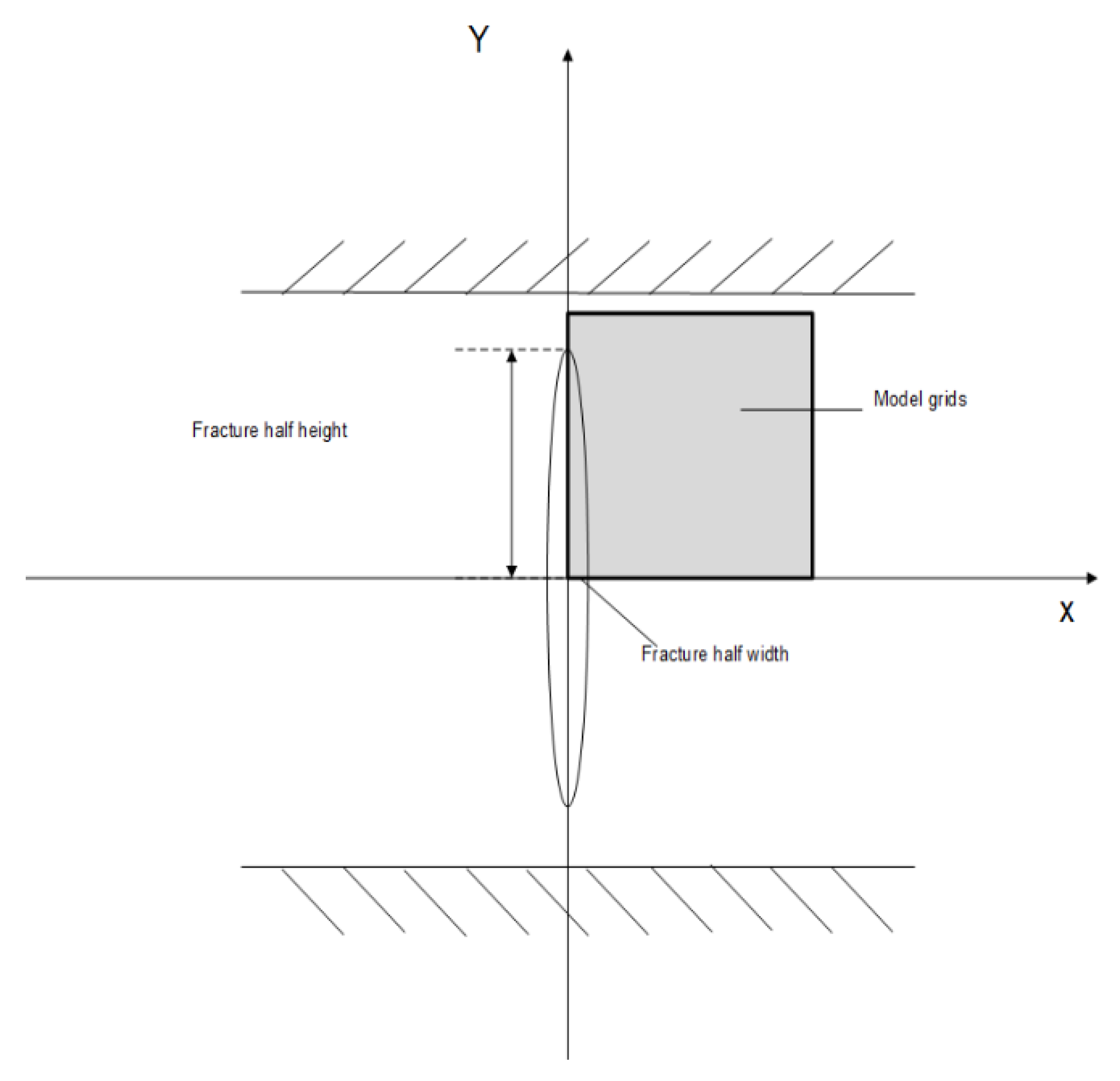
2. Model Description

The assumptions of the model are as follows: (1) The fracture geometry is plane-strain; (2) the fracturing fluid is incompressible, laminar, and Newtonian; (3) the lubrication theory can be applied for fluid flow calculation; (4) the linear elastic fracture mechanics theory is used as the criterion for fracture propagation; and (5) vertical stress is higher than the maximum horizontal stress. In addition, the M-integral method was used to calculate the stress intensity factor along the horizontal and vertical fracture propagation. Fracture tip stress intensity factors are first calculated as the fracture lengths propagate. Fracture height is then obtained for the in situ length when the stress intensity factor of the fracture tip in the vertical direction is equal to that in the horizontal direction.

2.1. Governing Equations

2.1.1. Mass Conservation

The fluid mass conservation law can be written as follows [26]:

$$\frac{\partial w}{\partial t}+\frac{\partial q}{\partial y}+C=0$$

(1)

where q is fluid flux, m³/min; w is fracture width, m; t is time, s; y is vertical flow direction; and $C$ is the leak-off term, m/s^0.5. Integrating Equation (1) twice yields the following:

$$2{{\displaystyle \int }}_0^{l}wdy+2{{\displaystyle \int }}_0^t{{\displaystyle \int }}_0^{l\left(t^{\prime }\right)}Cdy d{t}^{\prime }=Q_{0}t$$

(2)

2.1.2. Fluid Flow in the Fracture

Lubrication theory is used to describe fluid flow behavior within the fractures, which is described by the Poiseuille’s law:

$$q=-\frac{w^3}{12\mu }\left(\frac{\partial p_f}{\partial y}\right)$$

(3)

where $p_f$ is fluid pressure at the fracture surface, MPa; and $\mu$ is fluid viscosity, $\mathrm{Pa}\cdot \mathrm{s}$.

2.1.3. Fluid Leak-off

Carter’s leak-off model is used to describe fluid leak-off to the surrounding matrix (Carter, 1957):

$$C\left(y,t\right)=\frac{2C_l}{\sqrt{t-t_0\left(y\right)}},t>t_0\left(y\right)$$

(4)

where $C_l$ is leak-off coefficient, m/s^0.5; and $t_0\left(y\right)$ is the time the fracture tip arrives at position y, s.

2.1.4. Fracture Propagation Criterion

Tensile failure criterion is used for the reservoir rock to simulate fracture propagation, which is defined as follows:

$$K_I\ge K_{IC}$$

(5)

where $K_I$ is the stress intensity factor, $\mathrm{MPa}\cdot \sqrt{\mathrm{m}}$; and $K_{IC}$ is the critical stress intensity or fracture toughness, $\mathrm{MPa}\cdot \sqrt{\mathrm{m}}$.

2.1.5. Boundary Equations

Only a quarter of the fracture is modelled in this work, and the boundary conditions for fluid flow are as given below:

$$q\left(0\right)=\raisebox{1ex}{$Q_0$}\!\left/ \!\raisebox{-1ex}{$4$}\right.,q\left(l\right)=0$$

(6)

where $q\left(0\right)$ is fluid flux at the start of the crack, m³/min; and $q\left(l\right)$ is fluid flux at the fracture tip, m³/min; $Q_0$ is the total injection flow rate, m³/min.

2.1.6. Stress Intensity Factor Determination

The stress intensity factor $K_I$ is calculated with the M-integral method [27,28]. The M-integral method is a path-independent line integral that is applied to a class of plane elastic fracture problems for a variety of elastic crack problems:

$$K_I=\frac{E}{2\left(1-v^2\right)}\left\{\underset{D}{{\displaystyle \int }}\left[{\sigma }_{ij}\frac{\partial u_i{}^a}{\partial x_1}+{\sigma }_{ij}^a\frac{\partial u_i}{\partial x_1}-{\sigma }_{mn}^a{\epsilon }_{mn}{\delta }_{1j}\right]\frac{\partial \chi }{\partial x_j}dS-\underset{S_e}{{\displaystyle \int }}\chi p\frac{\partial u_i^a}{\partial x_1}dL\right\}$$

(7)

where domain D is a set of elements surrounding the fracture tip in the discretized finite element model. $S_e$ is a set of edges of the finite elements in domain D, and these edges coincide with the fracture surface; ${\sigma }_{ij}$ is the stress field; $x_j\left(j=1,2\right)$ is the local coordinate; $u_i\left(i=1,2\right)$ is the displacement field; $\delta$ is the Kronecker delta;$\chi$ is a scalar field; ${\epsilon }_{mn}$ is the strain field; ${\sigma }_{ij}^a$ and $u_i{}^a$ are the auxiliary stress and displacement field, respectively.

The auxiliary stress and displacement fields can be expressed as follows:

$$\left\{\begin{array}{c}{u}_1^a\\ u_2^a\end{array}\right\}=\frac{1}{2G}\sqrt{\frac{r}{2\pi }}\left\{\begin{array}{c}\cos \frac{\theta }{2}\left[\kappa -\cos \theta \right]\\ \sin \frac{\theta }{2}\left[\kappa -\cos \theta \right]\end{array}\right\}$$

(8)

$$\left\{\begin{array}{c}{\sigma }_{11}^a\\ {\sigma }_{22}^a\\ {\sigma }_{12}^a\end{array}\right\}=\frac{1}{\sqrt{2\pi r}}\cos \frac{\theta }{2}\left\{\begin{array}{c}1-\sin \frac{\theta }{2}\sin \frac{3\theta }{2}\\ 1+\sin \frac{\theta }{2}\sin \frac{3\theta }{2}\\ \sin \frac{\theta }{2}\cos \frac{3\theta }{2}\end{array}\right\}$$

(9)

where r is the distance from the fracture tip to the observation point x, and θ is the angle from the tangent to the fracture path. This angle equals $\frac{\pi }{2}$ as the fracture propagates in the vertical direction. In addition, $G$ is the shear modulus; κ is the Kolosov constant, where κ = (3 − ν) ∕ (1 + ν) for the plane stress condition, and κ = (3 − 4ν) for the plane strain condition.

2.2. Numerical Implementation

The equations discussed in the previous sections are coupled together to obtain an implicit solution for all equations. The finite element method was used in the simulation model. Fracture propagation for each time step is solved with a three-step process, described as follows:

A proper time step is assumed first, and then, the finite element discretization of the relationship between the fracture width w and the pressure in the fracture can be determined:

$$w\left(y,t\right)=\frac{\pi \left(1-{\upsilon }^2\right)}{4E}\underset{l\left(t\right)}{{\displaystyle \int }}\ln \left|\frac{\sqrt{l{\left(t\right)}^2-y^2}+\sqrt{l{\left(t\right)}^2-y_1^2}}{\sqrt{l{\left(t\right)}^2-y^2}-\sqrt{l{\left(t\right)}^2-y_1^2}}\right|p\left(y_1,t\right)d{y}_1$$

(10)

where $l\left(t\right)$ is the fracture half-height at time t.

The matrix form of equation of width and pressure is as follows:

$$\mathsf{\Delta }w=M\mathsf{\Delta }p$$

(11)

where $\mathsf{\Delta }w$ is width increment, m; and $\mathsf{\Delta }p$ is pressure increment, MPa; $M$ is pressure influence coefficient matrix; and the physical meaning of Mij is the fracture width at certain point i induced by unit pressure at another point j within the fracture. According to the principle of variation, Equation (1) with any test function leads to its weak form as follows:

$$\underset{L}{{\displaystyle \int }}\left[-\mathsf{\nabla }\left(\delta p\right)\cdot q+\left(\delta p\right)\frac{\partial w}{\partial t}+\left(\delta p\right)g\right]dl+\delta p\left(q\cdot n_1\right){|}_s=0$$

(12)

where $S$ is the collection of boundary conditions. Then, we can obtain the nonlinear finite equations and discretized equations.

An initial width w and pressure at time t are then assumed, and the Jacobian matrix generated in the process can be solved by a series of finite element equations. Backward Euler method is applied to solve the time difference in the integration. Newton–Raphson technique is conducted as the iteration method to solve the width and pressure increment in the next time step. $K_I$ is calculated by Equation (7) and compared with the fracture propagation criterion $K_{IC}$ (calculated based on the Brazilian test) in Equation (5). Such process is repeated until the solution converges.

Once the propagation criterion is met, the fracture propagates into the next grids, and fluid flows into the newly propagated fracture grid.

As the vertical stress is assumed to be the highest among all the stresses, fracturing fluid is assumed to flow in the vertical (y) direction in the early stage of the fracturing process. The model has 50 grids of 0.3 m in size in the vertical direction. In the horizontal (x) direction, grid size varies from 0.003 m at the fracture surface to several feet in the reservoir grids. Due to fracture symmetry, only a quarter of the fracture is modeled with half-length and half-width.

3. Fracture Height Calculation and Validation

3.1. Field Background

The Montney formation, located at the border of Alberta and British Columbia, Canada, is a sedimentary wedge that was deposited during the Early Triassic geologic period. Its lithology consists of interbedded fine-grained sandstones, siltstone, and dark gray shale. The reservoir depth ranges from 2800 m to 3500 m, reaching a maximum thickness of 280 m in the foothills of the northern Canadian Rockies and thinning out towards the north up to the Fort Nelson area and east to Peace River [29]. A large number of horizontal wells have been drilled in the heart of the Upper and Lower Montney gas plays [30]. The subject well is a horizontal well on the upper section of the Montney formation. A diagnostic fracture injection test (DFIT) was conducted before the well stimulation between the true vertical depth (TVD) of 2553 m and 2564 m.

Table 1. Parameters in the simulated well.

Parameters	Unit	Value
Minimum horizontal stress $\sigma$	MPa	44.2
Young’s modulus $E$	MPa	13,789.5
Poisson’s ratio $\upsilon$	/	0.2
Total injection flow rate $Q$	m3/min	2.9 × 10−3
Leak-off coefficient $C_l$	m/s0.5	1.5 × 10−5
Fluid viscosity $\mu$	mPa∙s	2.5

shows the key parameters associated with the DFIT operations.

3.2. Fracture Toughness Determination

Fracture toughness $K_{IC}$ is calculated based on the Brazilian test, which is a well-known indirect method used to measure rock tensile strength. The experiment is based on the observation that most rocks in biaxial stress fields fail due to tensile failure cracks along the loading diameter of the disc specimen [31].

The critical load in the experiment is shown as follows:

$$P_c=\frac{K_{IC}}{B\varphi \left(c/R\right)}$$

(13)

where $c$ is the fracture half-length, mm; $P_c$ is critical load, MPa; $R$ is radius of disc, mm; and B and $\varphi \left(c/R\right)$ are defined as follows:

$$B=\frac{2}{{\pi }^{3/2}{R}^{1/2}{t}_1\alpha }$$

(14)

$$\varphi \left(\frac{c}{R}\right)={\left(\frac{c}{R}\right)}^{1/2}{{\displaystyle \int }}_0^{c/R}\left[\varphi \left(\frac{r}{R}\right)/{\left(\frac{c^2}{R}-\frac{r^2}{R}\right)}^{1/2}\right]d\left(\frac{r}{R}\right)$$

(15)

where $t_1$ is the thickness of the disc (mm), and the value of the integral $\varphi \left(c/R\right)$ for a given $c/R$ can be estimated by a numerical integration method such as the Simpson’s method.

The values of the parameters in Equations (13)–(15) can be found in

Table 2. Parameters used for the $K_{IC}$ calculation.

Parameters	Unit	Value
Specimen’s angle $\alpha$	degree	5
Radius of disc $R$	mm	38
Thickness of the disc $t_1$	mm	47
Critical load $P_c$	kN	4.85
Integral $\varphi \left(\frac{c}{R}\right)$	/	0.112

, and $K_{IC}$ is calculated to be 0.244 $\mathrm{MPa}\cdot \sqrt{\mathrm{m}}$.

3.3. Numerical Model

A single fracture case was built via the finite element method, where only a quarter of fracture was simulated, as shown in Figure 1. The fracture grid was discretized into 50 cells with the size of 0.3 m in the vertical direction and varies from 0.003 m at the fracture surface to several feet in the horizontal direction to be compatible with the reservoir grids. The Young’s modulus, Poisson’s ratio, minimum horizontal stress, and fluid property values in the basic model are shown in the Table 1. In the basic model, a low-viscosity fluid (2.5 mPa∙s) was injected. In this model, when stress intensity factor in the vertical tip equals its value in the horizontal direction, the model stops, and the corresponding fracture heights will be calculated, after which the fracture mainly propagates in the horizontal direction, and the height of fracture stops increasing.

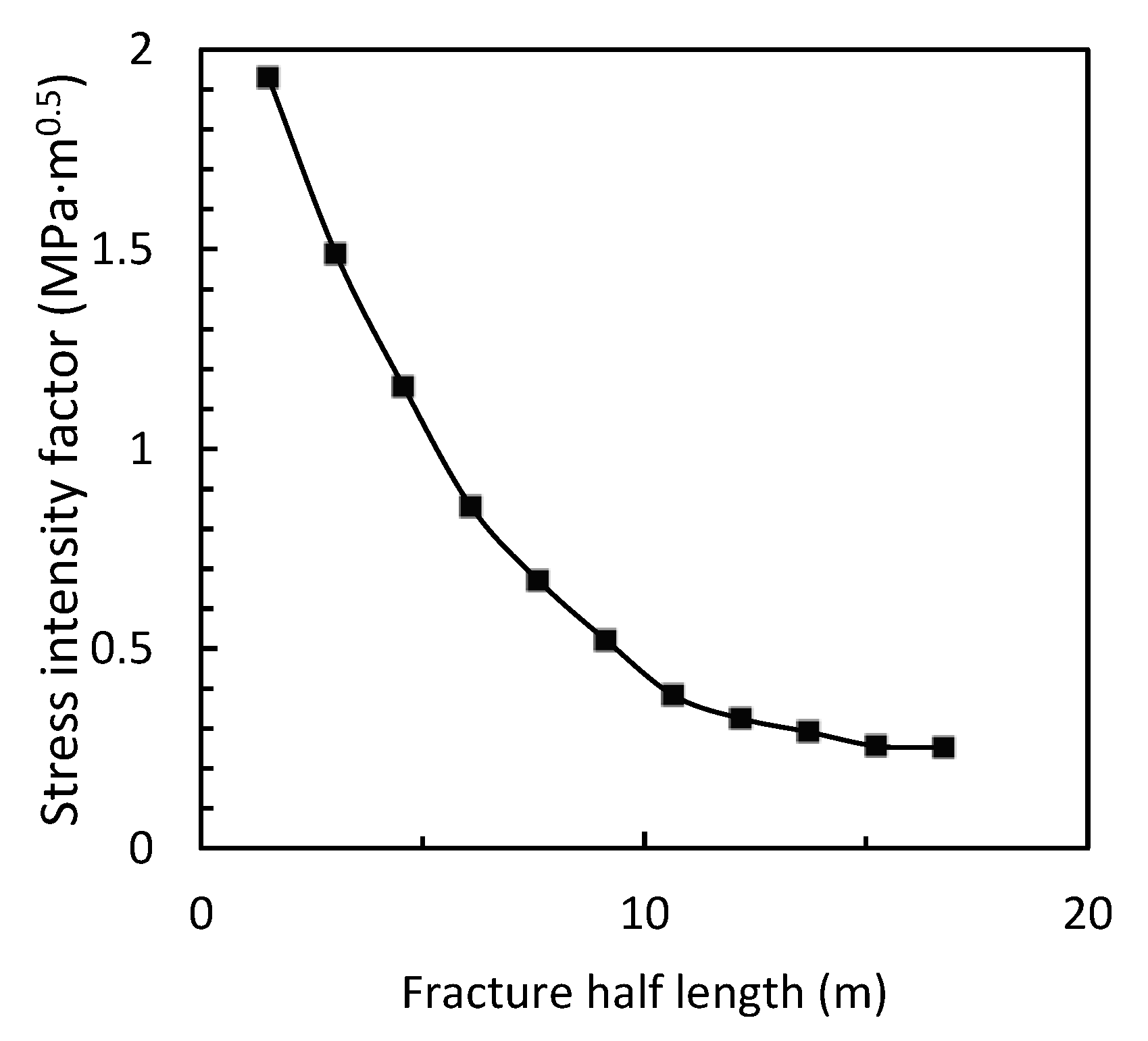
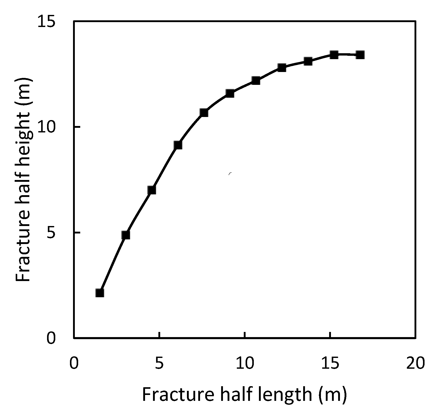
3.4. Fracture Height Calculation

As the fracture length propagates, stress intensity factor at the fracture tip under static condition is calculated by the M-integral method with the parameters $K_{IC}$ listed in Table 1. The relationship between the stress intensity factor and the fracture length is shown in Figure 2. The stress intensity factor decreases as the fracture half-length increases. When the fracture half-length reaches 16.8 m, $K_I$ decreases to 0.2520 $\mathrm{MPa}\cdot \sqrt{\mathrm{m}}$, which is slightly above the fracture toughness (0.2440 $\mathrm{MPa}\cdot \sqrt{\mathrm{m}}$).

While calculating fracture heights, $K_I$ under the different fracture half-lengths is used to replace $K_{IC}$. Specially, when the stress intensity factor in the vertical tip is equal to the critical stress intensity factor, the model stops, and the corresponding fracture heights will be outputted. We thus simulated the basic model with different half-fracture-lengths, and the calculated fracture heights and corresponding fracture lengths are shown in Figure 3.

Figure 3 shows that fracture propagates first in the vertical and horizontal directions simultaneously at a similar rate. Once the height reaches a certain value, the horizontal growth dominates the propagation. In other words, the fracture will mainly propagate in the horizontal direction while keeping the same height. For example, while the fracture half-length grows from 13.7 m to 15.2 m, the half-height of the fracture increases only from 13.1 m to 13.4 m. When the fracture half-length reaches 15.2 m, the height of the fracture stays at 13.4 m, and vertical propagation stops.

3.5. Reference Case

To compare with the results from analytical method, a simulation was run with our numerical model for 9 minutes’ fluid injection. The elastic modulus, Poisson’s ratio, minimum horizontal stress, and fluid property values in the basic model are the same as parameters in Table 1. The fracture half-length reaches 15.2 m at the end of the early fracturing process, after which the fracture will mainly propagate in the horizontal direction, and the height of fracture will stop increasing. The result is shown in Figure 4.

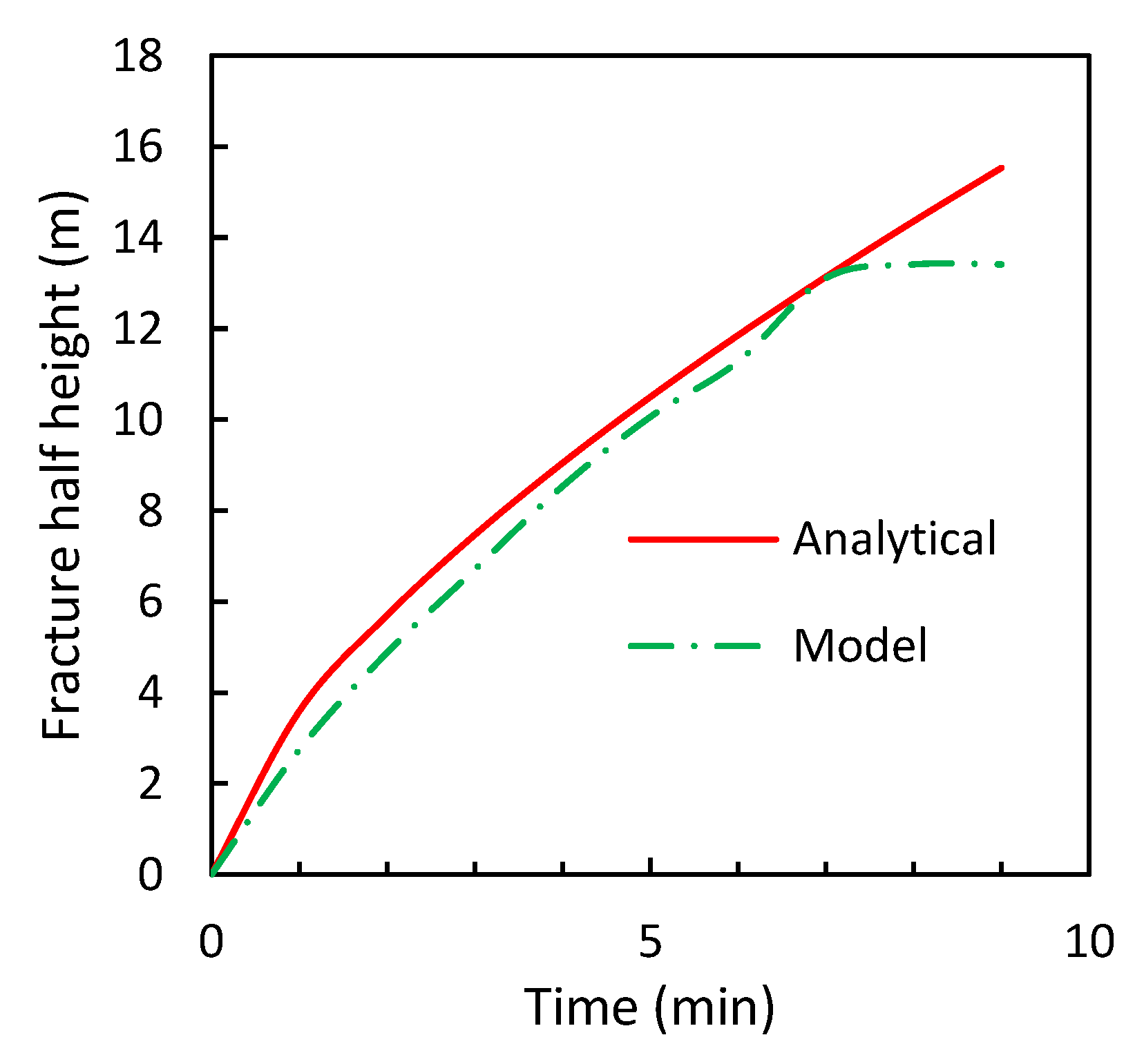
3.6. Analytical Case

An analytical model has been proposed in the literature where the pressure drop within the fracture is ignored, and the fracturing fluid is assumed to fill the entire fracture. An assumed fracture length is also required in the analytical model, and the fracture half-height could be calculated via the equation below:

$$H={\left(\frac{QEt}{\sqrt{\pi }\left(1-{\upsilon }^2\right)K_{IC}L}\right)}^{\raisebox{1ex}{$2$}\!\left/ \!\raisebox{-1ex}{$3$}\right.}$$

(16)

where Q is a quarter of the total injection rate at reservoir pressure, which is 0.00287 m³/min in this study, and L is the fracture half-length. It can be seen from Equation (16) that the fracture height is very sensitive to the fracture toughness. The fracture half-height is calculated to be 14.36 m after 9 min of injection.

Figure 4 compares the calculated fracture heights derived from the analytical model and the finite element method applied in this study. The dotted line represents fracture height using the finite element method, while the solid curve depicts calculated fracture height using the analytical model. The two calculated fracture half-heights are similar within the first 7 min. However, once the fracture height reaches 13.4 m, the model used in this study stops growing, while that of the analytical model continues to increase at the same rate. This is because the fracture length is assumed to be a constant value in the analytical model, and the fracture does not propagate in the horizontal direction. When the fracture length is given, the fracture would continue to propagate in the vertical direction. However, in fact, fracture propagation occurs in both vertical and horizontal direction, which is considered in this study. In the finite element model, the stress intensity factor is calculated for each time step and used as a key parameter to identify when the fracture propagation along the vertical direction stops. When the value of fracture tip toughness in the vertical direction is much larger than that of the horizontal direction, the fracture will stop extending in fracture height and focus on propagating in the horizontal direction. Fracture height will continue until the K_IC in both direction reaches equality in some certain time step.

3.7. Validation via Tracer Measurement

A radioactive tracer was run in the proppant stages of the treatment to measure the fracture height near the wellbore. The radioactive tracer was injected to measure the fracture height near the wellbore. The fracture treatments remain very restricted in the formation of interest with a fracture height of approximately 25 m (half-height is 12.5 m) [32]. The relative error of our model with real fracture height is 7.2%, indicating that the model is relatively accurate for fracture height calculation.

4. Sensitivity Analysis

This section discusses the characteristics of the response of the fracture height propagation and the effects of the main parameters on fracture height, including the grid size in the model, fluid viscosity, Young’s modulus, Poisson’s ratio, and minimum horizontal stress.

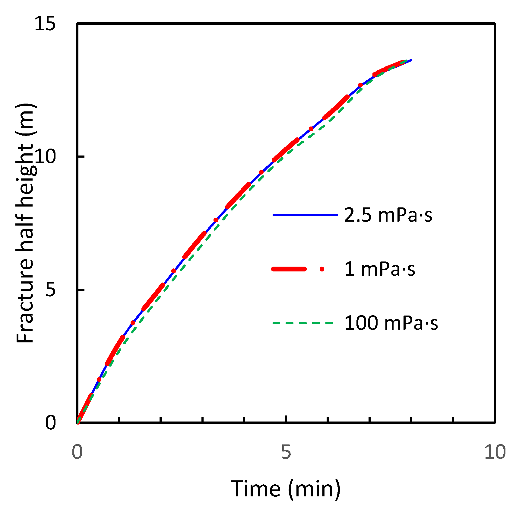
4.1. Fracturing Fluid Viscosity

The viscosity of the fracturing fluid affects pressure distribution along the fractures. Pressure drop within the fracture cannot be ignored, especially when the fracture length and/or height is long. Three fluid viscosities were studied in this work—1 $\mathrm{mPa}\cdot \mathrm{s}$, 2.5 $\mathrm{mPa}\cdot \mathrm{s}$, and 100 $\mathrm{mPa}\cdot \mathrm{s}$. The results are shown in Figure 5. Fracture height decreases slightly as the fluid viscosity increases. This is because a higher fluid viscosity leads to a higher pressure drop along the fracture and a lower fluid pressure at the fracture tip.

4.2. Reservoir Rock Properties

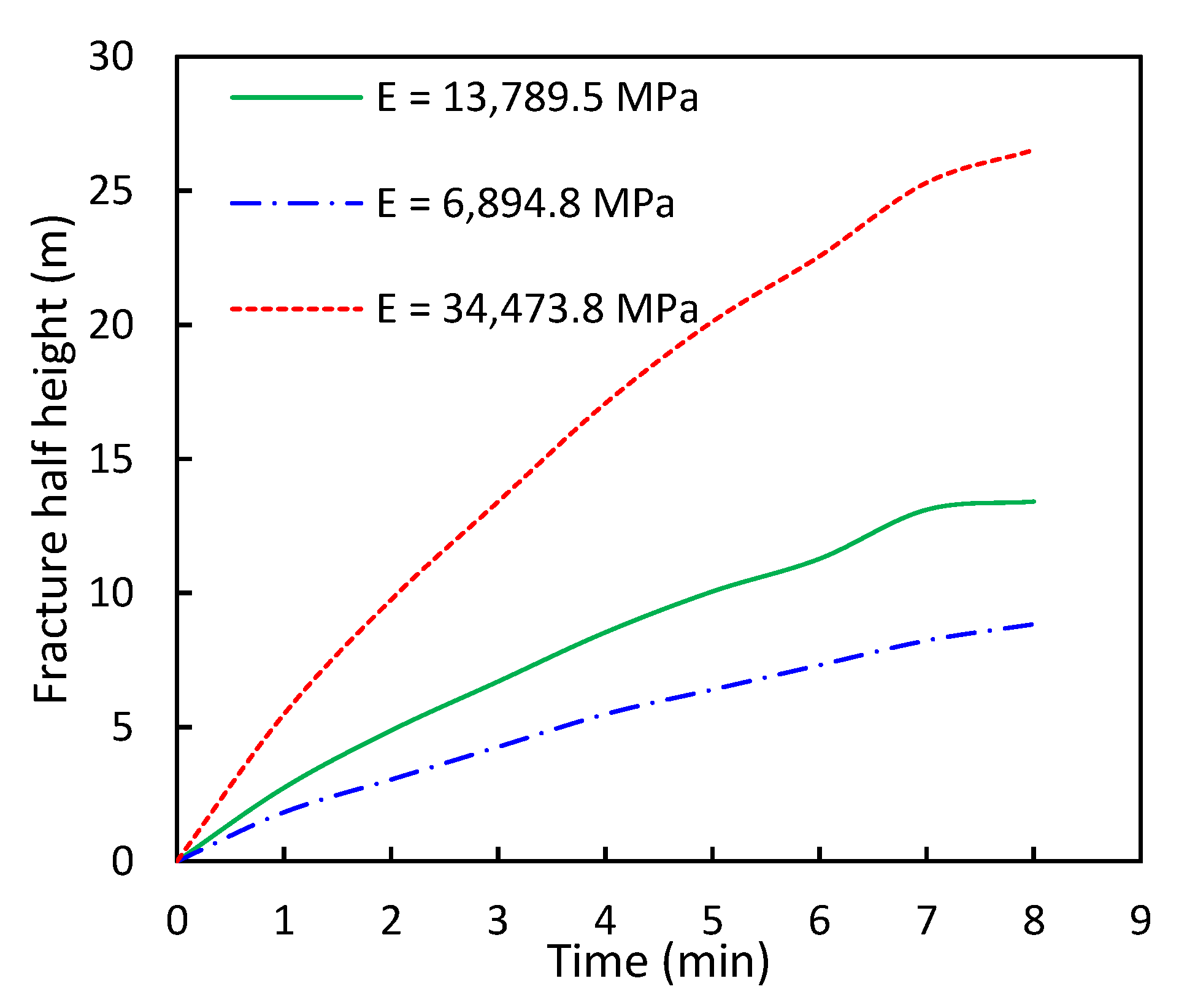
4.2.1. Young’s Modulus

Young’s modulus indicates the stiffness of the reservoir rock, and it affects the stress intensity factor calculated at the fracture tip. Three Young’s moduli were examined—13,789.5 MPa, 6894.8 MPa, and 34,473.8 MPa. Figure 6 depicts the fracture half-height calculated with the three Young’s moduli, respectively. The Young’s modulus can significantly affect the calculated half-height of the fracture. The higher the Young’s modulus, the larger the calculated fracture height will be. The calculated fracture half-height increased by nearly 100% when the Young’s modulus increased from 13,789.5 MPa to 34,473.8 MPa. This is because a high Young’s modulus leads to a large stress intensity factor at the fracture tip at each time step in the simulation, and thus, the fracture tends to propagate further into the formation. In addition, a large modulus indicates that the reservoir matrix is stiffer. Thus, the fracture propagates further, while the width of fracture tends to be narrower.

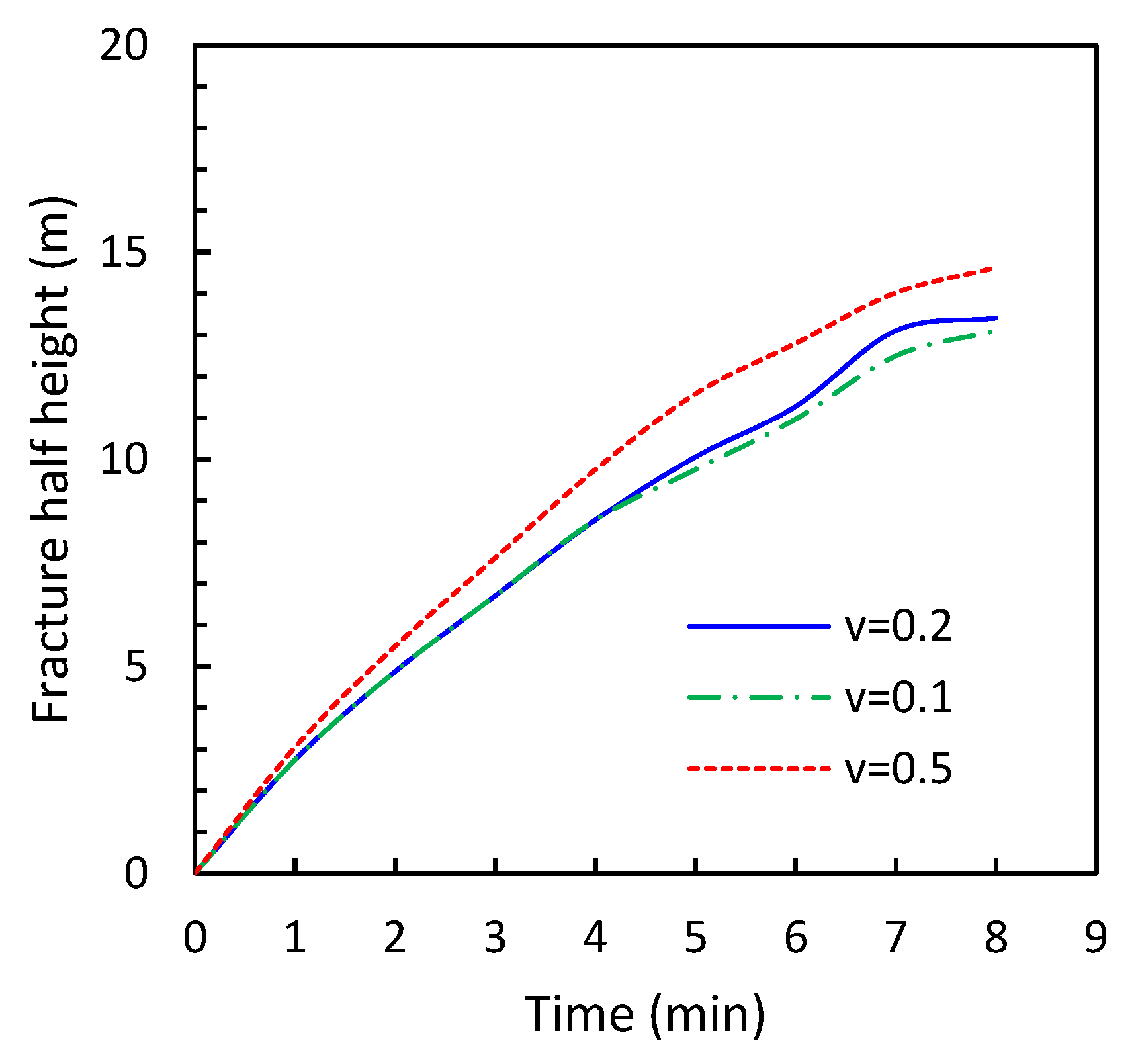
4.2.2. Poisson’s Ratio

The Poisson’s ratio is another key parameter that affects the stress intensity factor at the fracture tip. Three Poisson’s ratios—0.1, 0.2, and 0.5—were investigated in this study to evaluate its effect on fracture height. The results are shown in Figure 7, which demonstrates that a slight difference exists between scenarios when the Poisson’s ratios are 0.1 and 0.2, where the fracture half-height increases from 13.1 m to 13.4 m at the end of simulation. A noticeable difference is shown when the Poisson’s ratio increases to 0.5, where the calculated fracture half-height is increased to 14.6 m.

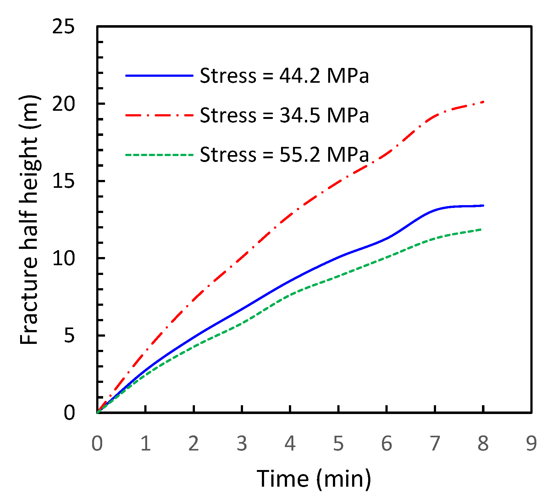
4.3. Minimum Horizontal Stress

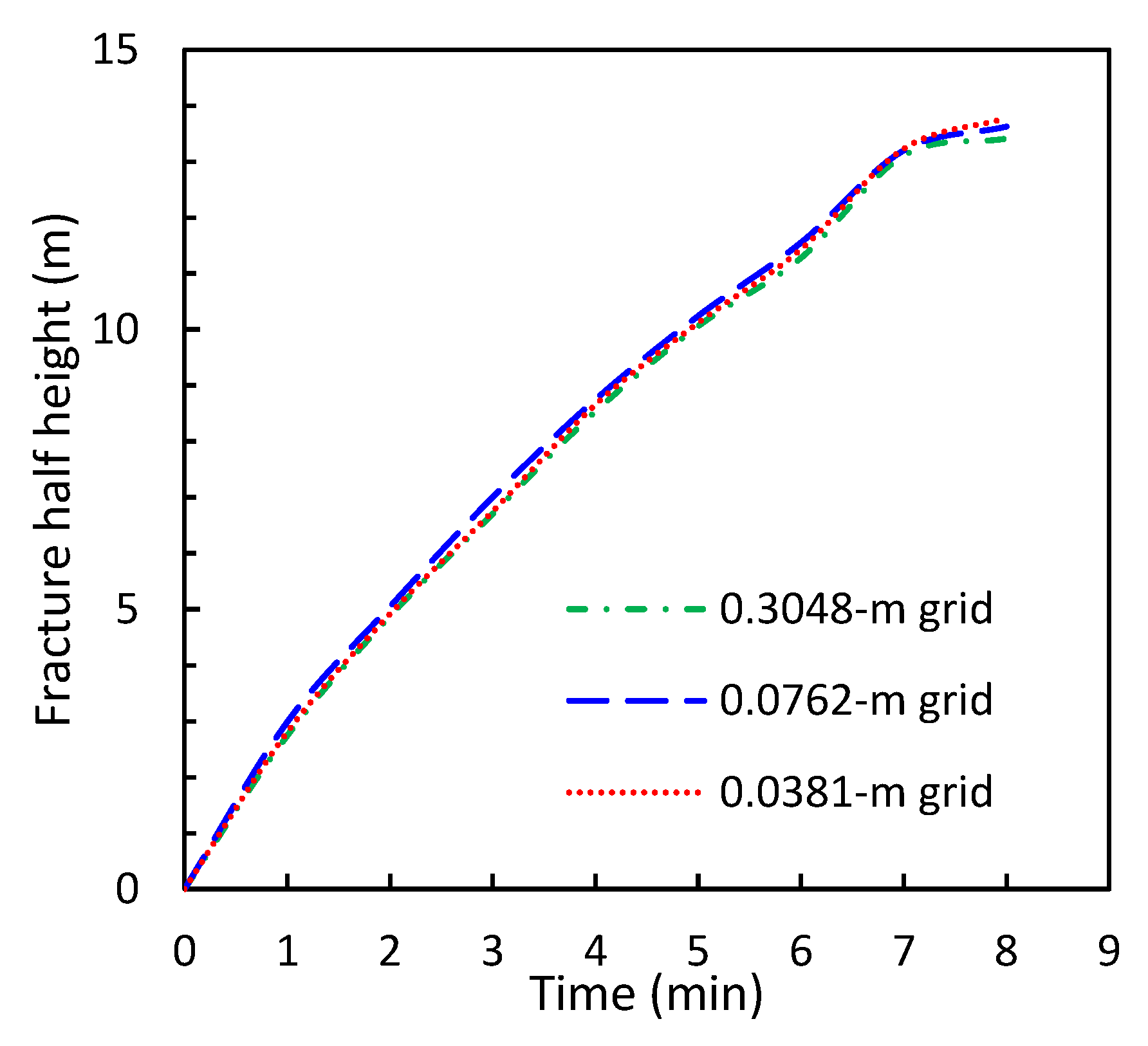
Minimum horizontal stress is an essential parameter to calculate the stress intensity factor at the fracture tip and the net pressure, which is the difference between fluid pressure in the fracture and rock stress on the fracture surface. Three minimum horizontal stresses of 34.5 MPa, 44.2 MPa, and 55.2 MPa were simulated in this study, and the results are shown in Figure 8. Calculated fracture height can be greatly affected by minimum horizontal stress. The fracture half-height reached 20.1 m for the scenario with a 55.2 MPa as the minimum horizontal stress compared to 13.4 m and 11.9 m for scenarios of 44.2 MPa and 34.5 MPa. The fracture propagates further under a smaller minimum horizontal stress. This is mainly because a lower minimum horizontal stress in the rock leads to a relatively large net pressure in the fracture and large stress intensity factor at the fracture tip.

4.4. Grid Size

In this study, fracture half-height is calculated to be 13.4 m with the vertical grid size of 0.3 m. To examine the sensitivity of the grid size to calculated half-height results, the model was repeated twice with a grid size of 0.075 m and 0.038 m in the fracture height direction. The results are shown in the Figure 9. A slight difference was found for the three grid sizes, indicating that 0.3 m of the grid size is sufficient for the calculation. With grid size changing from 0.3048m to 0.0762 m and 0.0381 m, the fracture half-height at the end of injection increased from 13.41 m to 13.62 m and 13.71 m. When the model grid is smaller, the dotted line of fracture half-height becomes smoother, but the influence of grid size on the fracture height is not significant.

5. Conclusions

• An innovative numerical model that fully couples the hydraulic fracture propagation, fluid flow in the fracture, and fluid leak-off into the reservoir matrix by finite element method is established to calculate fracture height in the tight formation using the proposed model;
• The well-based numerical model is successfully used in the filed case of Montney, which indicates a relative error of 7.2% compared with the field tracer result;
• The sensitivity analysis indicates that fracture height can be significantly affected by Young’s modulus and minimal horizontal stress. A high Young’s modulus leads to an increased stress intensity factor at the fracture tip for each time step, which prompts the fracture to advance further, while the width of fracture becomes smaller. The influence of grid size on height fracture is not significant. When the model grid is smaller, the trend of fracture height propagation becomes smoother.

References

1. Parshall, J. Barnett Shale showcases tight-gas development. J. Pet. Technol. 2008, 60, 48–55. [Google Scholar] [CrossRef]
2. Spellman, F.R. Hydraulic Fracturing Wastewater: Treatment, Reuse, and Disposal; CRC Press: Boca Raton, FL, USA, 2017. [Google Scholar]
3. Harrison, E.; Kieschnick, W.F., Jr.; McGuire, W.J. The mechanics of fracture induction and extension. Trans. AIME 1954, 201, 252–263. [Google Scholar] [CrossRef]
4. Howard, G.C.; Fast, C.R. Optimum fluid characteristics for fracture extension. In Drilling and Production Practice; American Petroleum Institute: Washington, DC, USA, 1957. [Google Scholar]
5. Crittendon, B.C. The mechanics of design and interpretation of hydraulic fracture treatments. J. Pet. Technol. 1959, 11, 21–29. [Google Scholar] [CrossRef]
6. Perkins, T.K.; Kern, L.R. Widths of hydraulic fractures. J. Pet. Technol. 1961, 13, 937–949. [Google Scholar] [CrossRef]
7. Nordgren, R.P. Propagation of a vertical hydraulic fracture. Soc. Pet. Eng. J. 1972, 12, 306–314. [Google Scholar] [CrossRef]
8. Khristianovic, S.; Zheltov, Y. Formation of vertical fractures by means of highly viscous fluids. In Proceedings of the 4th World Petroleum Congress, Rome, Italy, 6–15 June 1955; Volume 2, pp. 579–586. [Google Scholar]
9. Geertsma, J.; De Klerk, F. A rapid method of predicting width and extent of hydraulically induced fractures. J. Pet. Technol. 1969, 21, 1571–1581. [Google Scholar] [CrossRef]
10. Sneddon, I.N.; Elliot, H.A. The opening of a Griffith crack under internal pressure. Q. Appl. Math. 1946, 4, 262–267. [Google Scholar] [CrossRef]
11. Green, A.E.; Sneddon, I.N. The distribution of stress in the neighborhood of a flat elliptical crack in an elastic solid. In Mathematical Proceedings of the Cambridge Philosophical Society; Cambridge University Press: Cambridge, UK, 1950; Volume 46, pp. 159–163. [Google Scholar]
12. Simonson, E.R.; Abou-Sayed, A.S.; Clifton, R.J. Containment of massive hydraulic fractures. Soc. Pet. Eng. J. 1978, 18, 27–32. [Google Scholar] [CrossRef]
13. Fung, R.L.; Vilayakumar, S.; Cormack, D.E. Calculation of vertical fracture containment in layered formations. SPE Form. Eval. 1987, 2, 518–522. [Google Scholar] [CrossRef]
14. Warpinski, N.R.; Schmidt, R.A.; Northrop, D.A. In-situ stresses: The predominant influence on hydraulic fracture containment. J. Pet. Technol. 1982, 34, 653–664. [Google Scholar] [CrossRef]
15. Warpinski, N.R.; Teufel, L.W. Influence of geologic discontinuities on hydraulic fracture propagation (includes associated papers 17011 and 17074). J. Pet. Technol. 1987, 39, 209–220. [Google Scholar] [CrossRef]
16. Renshaw, C.E.; Pollard, D.D. An experimentally verified criterion for propagation across unbounded frictional interfaces in brittle, linear elastic materials. Int. J. Rock Mech. Min. Sci. Geomech. Abstr. 1995, 32, 237–249. [Google Scholar] [CrossRef]
17. Paris, P.C.; Sih, G.C. Stress analysis of cracks. In Fracture Toughness Testing and Its Applications; ASTM International: West Conshohocken, PA, USA, 1965. [Google Scholar]
18. Detournay, E. Propagation regimes of fluid-driven fractures in impermeable rocks. Int. J. Geomech. 2004, 4, 35–45. [Google Scholar] [CrossRef]
19. Sheibani, F.; Olson, J. Stress intensity factor determination for three-dimensional crack using the displacement discontinuity method with applications to hydraulic fracture height growth and non-planar propagation paths. In Effective and Sustainable Hydraulic Fracturing; InTech: Vienna, Austria, 2013. [Google Scholar]
20. Chen, Y.M. Numerical computation of dynamic stress intensity factors by a Lagrangian finite-difference method (the HEMP code). Eng. Fract. Mech. 1975, 7, 653–660. [Google Scholar] [CrossRef]
21. Pande, G.; Beer, G.; Williams, J. Numerical methods in rock mechanics. Int. J. Rock Mech. Min. Sci. 2002, 39, 409–427. [Google Scholar]
22. Olson, J.E.; Taleghani, A.D. Modeling simultaneous growth of multiple hydraulic fractures and their interaction with natural fractures. In Proceedings of the SPE Hydraulic Fracturing Technology Conference, The Woodlands, TX, USA, 19–21 January 2009. [Google Scholar]
23. Ma, D.; Duan, H.; Zhang, J.; Liu, X.; Li, Z. Numerical Simulation of Water–Silt Inrush Hazard of Fault Rock: A Three-Phase Flow Model. Rock Mech. Rock Eng. 2022, 55, 5163–5182. [Google Scholar] [CrossRef]
24. Ma, D.; Duan, H.; Zhang, J.; Bai, H. A state-of-the-art review on rock seepage mechanism of water inrush disaster in coal mines. Int. J. Coal Sci. Technol. 2022, 9, 50. [Google Scholar] [CrossRef]
25. Ma, D.; Duan, H.; Zhang, J. Solid grain migration on hydraulic properties of fault rocks in underground mining tunnel: Radial seepage experiments and verification of permeability prediction. Tunn. Undergr. Space Technol. 2022, 126, 104525. [Google Scholar] [CrossRef]
26. Boone, T.J.; Ingraffea, A.R. A numerical procedure for simulation of hydraulically-driven fracture propagation in poroelastic media. Int. J. Numer. Anal. Methods Geomech. 1990, 14, 27–47. [Google Scholar] [CrossRef]
27. Freund, L.B. Stress intensity factor calculations based on a conservation integral. Int. J. Solids Struct. 1978, 14, 241–250. [Google Scholar] [CrossRef]
28. Yau, J.F.; Wang, S.S.; Corten, H.T. A mixed-mode crack analysis of isotropic solids using conservation laws of elasticity. J. Appl. Mech. 1980, 47, 335–341. [Google Scholar] [CrossRef]
29. Dembicki, M.; Nevokshonoff, G.; Johnsen, J.; Spence, M. The super pad—A multi-year integrated approach to resource development in the montney. In Proceedings of the Unconventional Resources Technology Conference, San Antonio, Texas, 20–22 July 2015; Society of Exploration Geophysicists: Tulsa, OK, USA; American Association of Petroleum Geologists: Tulsa, OK, USA; Society of Petroleum Engineers: Houston, TX, USA; pp. 2684–2695. [Google Scholar]
30. Stevens, S.; Ruuskraa, V. Special report: Gas shale-1: Seven plays dominate North America activity. Oil Gas J. 2009, 29, 36–41. [Google Scholar]
31. Aziz, N.I.; Schmidt, L.C. Rock fracture-toughness determination by the Brazilian test. Eng. Geol. 1993, 33, 177–188. [Google Scholar]
32. Popp, M. Completion and Stimulation Optimization of Montney Wells in the Karr Field. Ph.D. Thesis, University of Calgary, Calgary, AB, Canada, 2015. [Google Scholar]
Figure 1. Schematic diagram for a hydraulic fracture in the tight formation.
Processes 11 01566 g001
Figure 2. Change of the stress intensity factor as fracture half-length propagates.
Processes 11 01566 g002
Figure 3. Propagation of the fracture half-height as the fracture half-length extends.
Processes 11 01566 g003
Figure 4. Fracture heights propagation with time.
Processes 11 01566 g004
Figure 5. Fracture heights sensitivity to fluid viscosity.
Processes 11 01566 g005
Figure 6. Fracture half-heights’ sensitivity to Young’s modulus.
Processes 11 01566 g006
Figure 7. Fracture half-heights’ sensitivity to Poisson’s ratio.
Processes 11 01566 g007
Figure 8. Fracture half-heights’ sensitivity to minimum horizontal stress.
Processes 11 01566 g008
Figure 9. Fracture half-heights’ sensitivity to grid size.
Processes 11 01566 g009