1. Introduction
In recent years, with the sustained growth of the global economy, energy consumption has risen sharply. This phenomenon has led to exacerbated global air pollution, severe ecological damage, and an increasing threat to global sustainable development. For example, the rising demand for energy has resulted in the burning of large amounts of fossil fuels, which releases significant amounts of carbon dioxide and other greenhouse gases, accelerates the pace of climate change, and has a serious impact on the ecological environment, such as by causing increased extreme weather events and declining biodiversity. Therefore, it is necessary to propose solutions to address this issue in order to achieve global sustainable development goals. Governments have become increasingly concerned about the problem of carbon dioxide (CO2) emissions. The Intergovernmental Panel on Climate Change (IPCC) enacted the United Nations Framework Convention on Climate Change (UNFCCC) in 1992 as the first global agreement aimed at comprehensively controlling greenhouse gas emissions, taking into account CO2 emissions. Subsequently, the global community established a series of international conventions, including the Kyoto Protocol and the Paris Convention, in an effort to mitigate the disasters stemming from global warming.
Crude oil ranks among the primary energy sources on the global scale and its price movements have a significant impact on the global economy. It is an essential product for industrial production and a crucial raw material for gasoline, diesel, and lubricating oil used in transportation. Many daily necessities rely on the extraction and manufacture of crude oil because crude oil is connected to human economic conditions and the day-to-day lives of citizens countries around the world pay close attention to the economic impacts caused by oil crises and political factors [
1,
2,
3,
4,
5]. Due to the inseparable relationship between crude oil and the economy, many countries highly rely on it, resulting in increased CO
2 emissions and making it a major contributor to global warming. In 2016, BP published a report on countries that are highly dependent on crude oil, ranking them in the following order: the United States, China, India, Japan, and Saudi Arabia [
6]. Renewable energy is an alternative to reliance on crude oil, e.g., electric vehicles.
It is widely agreed that petroleum consumption is one of the major causes of CO
2 emissions. The effects include land and ocean pollution caused by accidental leaks and pipeline ruptures, as well as upstream industry activities such as oil well drilling, production, transportation, and storage, and downstream activities such as refining, transportation, and sales [
7,
8]. In addition, the indiscriminate disposal of waste products from crude oil refining can also pollute the environment. The continued burning of fossil fuels has already caused the release of over 75% of CO
2 emissions into the aerosphere, leading to depletion of the Earth’s ozone layer and extreme weather phenomena such as El Niño, resulting in frequent global disasters [
9,
10].
As crude oil represents the largest proportion of primary energy sources, it inevitably contributes to major environmental damage through, e.g., CO
2 emissions. The International Energy Agency (IEA) notes that the ongoing surge in CO
2 emissions resulting from crude oil is a substantial factor in the amplification of global warming and the regular occurrence of natural disasters, and the increasing use of renewable energy sources has yet to offset this trend [
11]. However, the impact of CO
2 emissions varies considerably among countries that export and import oil [
12]. As an illustration, Alshehry and Belloumi [
13] explored the environmental Kuznets curve (EKC) theory [
14] in Saudi Arabia between 1971 and 2011 and found no indication of an inverted U-shaped link between CO
2 emissions from oil transportation and economic growth [
15]. This indicates that crude oil exporting countries do not necessarily increase their CO
2 emissions due to economic growth. However, taking Pakistan as an example, Rahman and Ahmad [
16] identified that coal and crude oil consumption play a crucial role in CO
2 emissions, and proved that there is an inverted U-shaped correlation in both the long run and the short run under the extended EKC theory [
17]. This indicates that crude oil importing countries tend to experience a decrease in CO
2 emissions after an initial increase due to economic growth. Similarly, in developing countries such as Bangladesh, which have no renewable energy sources, crude oil, natural gas, and refined oil are the major resources for the transportation sector, power production, and manufacturing plants, and there is a close correlation between the depletion of such energy inputs and CO
2 emissions [
18].
There are many reasons for the increase in CO
2 emissions beyond petroleum consumption, including Bitcoin, which is based on blockchain technology. Given that Bitcoin has the largest market share in the cryptocurrency market as the top virtual currency, we suspected that there might be a connection between crude oil and Bitcoin, with Bitcoin representing a vital factor. Due to its decentralized nature, its price and trading volume are influenced by many factors. Some studies have shown that the price fluctuation of Bitcoin and crude oil have a two-way interrelation. For example, Jin et al. found a two-way spillover effect between oil and Bitcoin [
19,
20]. Bouri et al. found a significant connection between oil shocks and Bitcoin volatility, verifying the existence of a causal relationship over time at different time scales [
21,
22]. Jareño et al. confirmed that crude oil and cryptocurrency are more interdependent in times of economic turmoil [
23,
24,
25,
26,
27]. Wang et al. found that the cryptocurrency environment attention index (ICEA) shows a significant positive correlation between Brent crude oil and Bitcoin [
28]. Notably, a drastic reduction in the price of Bitcoin substantially affects the price of crude oil, with a noticeable impact on oil exporting countries [
29]. Due to factors such as geopolitical events, production supply constraints in oil-producing countries, natural disasters, etc., the crude oil market can experience price volatility. Investors may seek decentralized and non-traditional markets, with factors influenced by Bitcoin as a hedge tool to mitigate the risks. However, Bitcoin’s hedging properties do not just depend on market conditions, but also on various types of oil price trends. Selmi et al. used quantile regression to suggest that gold and Bitcoin can act as refuges in the crude oil market during turbulent times [
30,
31]. To our knowledge, there has not yet been any systematic investigation into the correlations among crude oil, Bitcoin, and CO
2 emissions across time periods.
Bitcoin is strongly correlated with CO
2 emissions. The process of mining Bitcoin requires a significant amount of electricity and computing power, which has a negative effect on the environment. As Bitcoin becomes more popular, its environmental damage is a worrying concern. Moreover, Bitcoin’s high energy consumption and CO
2 emissions also raise questions about the sustainability of cryptocurrency. The interrelation between Bitcoin and crude oil is reflected in the fact that Bitcoin mining uses a considerable amount of energy, and both require a lot of energy [
32,
33]. According to a 2017 report by China’s National Bureau of Statistics (NBSC), the crude oil refining sector accounts for 12.5% of the country’s power consumption. The CO
2 emissions from the crude oil refining industry involve the generation of electricity, steam, and heat [
11]. Similarly, Bitcoin is a power-hungry entity, with annual power consumption for mining exceeding the electricity usage of Argentina, Austria, and Cyprus, and its CO
2 emissions equivalent to the average level of Kansas City [
34,
35,
36,
37,
38,
39,
40]. It is expected that in China, Bitcoin energy consumption will result in 130.5 million tons of CO
2 emissions by 2024, exceeding the total annual carbon emissions of both Qatar and the Czech Republic [
41]. In simpler terms, cryptocurrency mining contributes to the rise in energy consumption and the generation of CO
2 emissions from mining-related pollution [
41,
42]. Studies have suggested that Bitcoin’s energy consumption and carbon footprint are directly related to its transaction volume, with an increase in transaction volume causing a dynamic impact, leading to a 46.54% upsurge in its energy depletion and carbon footprint [
43,
44,
45,
46,
47]. To address this issue, China banned cryptocurrency mining in 2021, leading to approximately half of the global miners migrating to neighboring countries such as Iran and Kazakhstan. While CO
2 emissions immediately decreased in China, the problem shifted to those other regions and resulted in increased CO
2 emissions there [
48]. The CO
2 emissions generated by cryptocurrency mining cause significant harm to the environment.
If CO2 emissions can be effectively reduced, the benefits to the global climate and the environment will be significant. This study argues that studying the relationship among crude oil, Bitcoin, and CO2 emissions can help to deepen our understanding of their complex interactions. While there has been considerable discussion on the interrelation between crude oil and CO2 emissions, crude oil and Bitcoin, or Bitcoin and CO2 emissions, there has been no research on the relationship among all three, with Bitcoin acting as the mediating variable.
The aim of this study was to analyze the direct or indirect relationship, or coexistence of both, between crude oil and CO2 emissions through Bitcoin. Quantile regression was employed to determine whether there is an inverted U-shaped nonlinear correlation between crude oil and CO2 emissions, and between Bitcoin and CO2 emissions. In addition, we also investigated whether Bitcoin has a moderating intermediate effect.
This study provides an innovative approach, adapting the mediation analysis approach proposed by Baron and Kenny [
49] and Koenker and Bassett [
50] with quantile regression. This approach can explore the dynamic causal effect of crude oil on CO
2 emissions in the short term, regardless of its correlation with Bitcoin volatility. The objective is to achieve the goal of decreasing CO
2 emissions based on exploring the relationships between them. Quantile regression models are highly advantageous due to their exceptional robustness, eliminating the need to make any presumptions about the distribution of error terms [
51,
52]. In addition, compared to traditional ordinary least squares (OLS) regression, which only explores the conditional expected value of the explanatory variable, quantile regression investigates the full range and conditional allocation of the response variable’s median. Furthermore, the effect of the explanatory variable on the response variable fluctuates across quantiles, resulting in a more detailed and effective approach.
2. Methodology
The new approach proposed in this paper blends mediation analysis and quantile regression to explore the effect of crude oil on CO2 emissions, with or without the effect of Bitcoin volatility, providing a unique perspective on the correlation between these variables. The results can serve as a reference for governments of various countries, or the Taiwanese government, in formulating energy-saving and carbon reduction policies.
Our data cover a total of 1826 observations from 1 January 2018 to 31 December 2022. To ensure cross-sectional consistency, we relied on the Investing.com database to provide us with daily market closing prices of Brent crude oil, Bitcoin, and carbon emission futures, which were used to create a logarithmic model.
2.1. Chow Test
The Chow test is used to test whether the regression coefficients of two different sets of data are equal. It is widely used to test for the existence of structural changes in time series [
53]. The main purpose is to test for statistically significant differences between two or more regression models, making it particularly suitable for detecting the presence of structural breaks in time series data. The calculation uses the following equation (Equation (1)):
If our data model is Y = a + b X1 + c X2 + ε, we divide the data into two groups:
Data set 1. Y1 = a1 + b1 X1 + c1 X2 + ε
Data set 2. Y2 = a2 + b2 X1 + c2 X2 + ε
H0. a1 = a2, b1 = b2, and c1 = c2 are structurally similar for data sets 1 and 2.
H1. At least one of a, b, and c is structurally different for data sets 1 and 2.
Critical value: Fα,k,n−2(k + 1)
Rejection rule: F > Fα,k,n−2(k + 1), thus we can reject H0.
In the above equation, SSRpooled is the residual sum of squares of the merged data, SSR1 is the residual sum of squares of the first group of data, SSR2 is the residual sum of squares of the second group of data, n is the number of observations in the merged regression, and k is the total number of variables.
2.2. Augmented Dickey–Fuller (ADF) Unit Root Test
Non-stationarity is a common occurrence among time series variables. To address non-stationary time series, the general strategy is to transform them into stationary series and then use stationary time series methods to investigate them. An approach for assessing the stationarity of a time series is to detect its unit root. When a non-stationary time series possesses a unit root, the next step is to difference it to eliminate the unit root, which produces a stationary time series. Unit root testing is the basis for discussing the existence of cointegration and the persistence of sequence volatility.
To begin with, we utilize the augmented Dickey–Fuller (ADF) unit root model to perform a test, which primarily involves estimating α [
54,
55]. Using Equation (2), we can test the alternative hypothesis for α < 0, while the null hypothesis is α = 0:
where ∆ represents first-order differencing, y
t is the tested time series, t is the time trend variable, k is added to account for the lag of the residual, and ε
t is white noise. When the null hypothesis is not rejected, it indicates that the sequence is non-stationary, and when the null hypothesis is rejected, it implies stationarity of the time series.
2.3. Johansen Cointegration Test
Pagan and Wickens pointed out that if a single variable has a unit root, further cointegration tests are required [
56]. When time series exhibit a cointegration relationship, it implies that the variables may display short-term fluctuations but will eventually move toward equilibrium in the long term. As long as there is a cointegration relationship, the variables do not need to be treated with first-order differencing [
56]. Therefore, our testing method adopts the trace test of the Johansen cointegration test [
57,
58,
59], as shown in Equation (3):
where, T is the sample number,
is the estimate of the ith eigenvalue in the matrix, and r is the number of cointegrated vectors. If there are r sets of co-integrated vectors, then λ
1 ≠ 0, λ
2 ≠ 0, …, λ
i ≠ 0, and the trace value must be greater than the critical value of 5%.
2.4. Quantile Regression
Generally speaking, regression analysis is limited to estimating the mean or average of the response variable pursuant to the explanatory variables. However, Koenker and Bassett [
50] proposed quantile regression, which can be used to further infer the conditional assignment of the response variable. This method can replace ordinary least squares (OLS) regression. This approach for estimating the conditional quantile function can more comprehensively describe the influence of various explanatory variables, rather than being limited to the conditional expected value. Therefore, quantile regression is widely used in various fields, such as ecology, healthcare, and financial economics. This approach was later extended by Koenker, Hallock, and Koenker [
51,
52]. Referring to Koenker [
52], quantile regression can estimate any quantile, including the median and other conditional quantiles, and even the entire range of the distribution, rather than using OLS to estimate the mean.
In addition, quantile regression has four distinct advantages. First, it does not have to make assumptions for error terms, which helps to resist the influence of outlier observations. Second, if the error term is not non-normal or the variable distribution deviates significantly from normal or contains outliers, it is a more effective method than OLS. Third, because it describes both statistical dispersion and central tendencies, it responds more robustly to larger outliers, which helps to analyze the relationship between variables more comprehensively. Finally, it is possible to estimate any quantile if there are sufficient data.
We followed Koenker and Bassett’s approach [
50], and present the regression process as shown in Equation (4), where y
t, t = 1, 2, 3, …, T represents a stochastic sample that is used in the following regression process:
Equation (5) has a conditional distribution function, given by:
Equation (6) evaluates the marginal impact of an explanatory variable on the response variable through the θth quantile regression Q
y/x (θ), where 0 < θ < 1. In this quantile regression, x
t, t = 1, 2, 3, …, T represents a queue of k rows of vectors for a given model matrix. The model estimates the effect of an explanatory variable on the response variable under a particular conditional component, and represents the minimization of the θth quantile regression as follows:
The solution to this problem is βθ, which corresponds to the θth conditional quantile, Qy/x (θ) = xβθ.
2.5. Meditation Analysis of Bitcoin
According to Baron and Kenny’s approach, the mediating effect is an important mechanism between the explanatory and response variables. To employ mediation analysis using our data, we investigated the potential causal pathways linking crude oil volatility and CO
2 emissions via Bitcoin, and the direct correlation between crude oil and CO
2 emissions. Following Baron and Kenny’s causal steps procedure [
49], by examining the mediating variable, we can demonstrate a relationship between the explanatory and response variables, and construct the following regression equations (Equations (7)–(9)):
Here, BRT refers to Brent crude oil price representing the explanatory variable of crude oil; BTC refers to Bitcoin price representing the mediating variable of Bitcoin volatility; CO2 refers to carbon emission futures price representing the response variable of CO2 emissions; and ei, i = 1,2,3 refers to random error terms.
In addition, according to Baron and Kenny’s proposition [
49], the mediating variable between the explanatory and response variables must satisfy three conditions: there must be (1) a significant interrelationship between the explanatory variable and the mediating variable; (2) a significant interrelationship between the mediating variable and the response variable; and (3) a decrease in strength of the direct relationship between the explanatory and response variables after adding the mediating variable. Therefore, our mediation analysis of Bitcoin volatility includes the following steps:
Step 1: The explanatory variable BRT should be correlated with the response variable CO2 such that b1 is significant in Equation (7). This confirms a significant relationship between BRT and CO2.
Step 2: The explanatory variable BRT should be correlated with the mediator variable BTC such that c1 is significant in Equation (8). This represents the first stage in our establishment of mediation effects.
Step 3: The mediator variable BTC should be correlated with the response variable CO2 such that d2 is significant in Equation (9). This represents the second stage in our establishment of mediation effects. Step 4: After controlling for the mediating variable BTC, the explanatory variable BRT should no longer be correlated with the response variable CO2, such that d1 is non-significant in Equation (9). At this point, when considering the mediating effect transmitted through BTC, the relationship between BRT and CO2 checked in step 1 disappears, indicating the complete mediating effect of BTC. Nevertheless, if d1 in Equation (9) is still significant and less than b1 in Equation (7), that is d1 < b1, then BTC exhibits a partial mediating effect.
2.6. Quantile Meditation Analysis
According to the integrated approach proposed by Hsu [
60,
61], we blended quantile regression with mediation analysis by incorporating Equation (6) into Equations (7)–(9) and obtained Equations (10)–(12), which explain minimizing the sum of weighted errors in a quantile mediation regression.
By enabling the examination of all possible parameters (across all quantiles), which can differ based on the response variable’s level, this approach complements the standard regression estimate, which exclusively takes into account a single b, c, or d value. This novel approach helps in comprehensively understanding the dynamic relationship between BRT and CO2, as well as their causal relationship.
2.7. Environmental Kuznets Curve (EKC)
The environmental Kuznets curve (EKC) hypothesizes that market forces will initially increase and then decrease economic inequality with economic development, exhibiting an inverted U-shaped curve [
14].
As most of the literature illustrates a causal relationship between Bitcoin returns and global economic policies [
62,
63,
64,
65,
66,
67], this study adopts a quantile regression model and constructs a non-linear model based on Equations (13) and (14), as proposed by Grossman and Krueger [
68], which analyzes whether there is an inverted U pattern between CO
2 and crude oil or Bitcoin.
At specific quantiles of CO
2 emissions, Equations (13) and (14) require testing the null hypothesis that α
1 and β
1 are greater than zero, and α2 and β2 are less than or equal to zero. If the
p-value obtained from the t-value calculation is less than 0.05 for these equations, this suggests the presence of a significant inverted U-shaped curve [
68].
3. Results
In this study, we relied on the Investing.com database to provide daily market closing Brent crude oil spot prices (in USD per barrel), Bitcoin prices (in USD per Bitcoin), and carbon emission futures prices (in EUR per metric ton) to create a logarithmic model. The data cover a total of 1826 observations from 1 January 2018 to 31 December 2022. We used EViews12 software to perform descriptive statistics to summarize and characterize the data, in order to understand the overall distribution of the data.
Table 1 outlines the descriptive statistics in summary form. Only the kurtosis coefficient of BRT is greater than 3, exhibiting a leptokurtic phenomenon, and the skewness coefficient shows a left-skewed phenomenon. The Jarque–Bera test indicates that all variables have non-normal distribution. Bitcoin has a standard deviation of 0.359, indicating higher volatility than Brent crude oil and CO
2 emissions.
Figure 1 displays volatility plot for these variables, with a clear breakpoint observed for CO
2 emissions on 18 March 2020. Therefore, we used the Chow breakpoint test to confirm the existence of a structural break.
The F-value obtained in the Chow breakpoint test was 1019.141, which rejects the null hypothesis and indicates that 18 March 2020 was a structural breakpoint during the research period. In other words, there was a structural change in the impact of crude oil and Bitcoin on CO2 emissions after that date. This coincided with the initial outbreak of COVID-19, when countries such as China and Italy began to implement lockdown measures.
As shown in
Table 2, the linear regression indicates that before COVID-19, crude oil and Bitcoin had a reverse effect on CO
2 emissions. However, after COVID-19, crude oil had a positive effect and Bitcoin had a reverse effect on CO
2 emissions.
To establish the integration order of BRT, BTC, and CO
2 prior to estimating Equations (10)–(12), we utilized the ADF unit root test [
55].
As shown in
Table 3, the unit root hypothesis was rejected for all three variables, with the significance level set at 1%. This indicates that all variables have a unit root unless they are differenced once, and the hypothesis of a unit root is not supported by the data, with the significance level set at 1%. Therefore, we further conducted a cointegration test, which indicates that if a cointegrating relationship is present, the variables fluctuate differently in the short term but tend to balance in the long term, and do not need to be first-differenced [
57,
58,
59].
Table 4 lists the outcomes of best lag length after the cointegration test. While the SC and HQ criteria lag behind by 1 and 2 periods, respectively, the other two criteria lag behind by 8 periods. Since the sample size is 1826, which is considered a large sample from the time series perspective, and based on the principle that smaller lag length is better, the SC criterion with a lag length of 1 is suitable.
Table 5 shows that there is one cointegrating relationship, and the findings suggest that crude oil, Bitcoin, and CO
2 emissions are interconnected, with a common long-term trend, and tend to return to an equilibrium state, even after experiencing significant short-term deviations. Therefore, the variables do not need to be first differenced [
57,
58,
59].
Table 6 lists the outcomes of causality tests for BRT, BTC, and CO
2. For Equations (10) and (11), we find the following results. Traditional OLS and quantile regression across different CO
2 emission distributions provides evidence of a causal relationship between BRT and CO
2. Through quantile regression, a direct correlation is found between BRT and CO
2 emissions, except at the 10th percentile of CO
2 emission distribution. The results indicate that the influence of BRT on CO
2 emissions differs across the quantiles of distribution, with a more significant effect at the upper quantiles (see
Table 6 and
Figure 2).
Additionally, using traditional OLS and quantile regression (
Table 6) reveals a causal relationship between BRT and BTC across different quantiles distribution. The results indicate a significant positive impact of BRT on BTC across the entire range (see
Table 6 and
Figure 3). These results set up the first stage of the mediating effect of BTC.
The x-axis indicates CO2 quantiles and y-axis indicates BRT coefficient values. The orange line indicates estimated 95% confidence interval for quantiles.
The x-axis indicates BTC quantiles and the y-axis indicates BRT coefficient values. The orange line indicates estimated 95% confidence interval for quantiles.
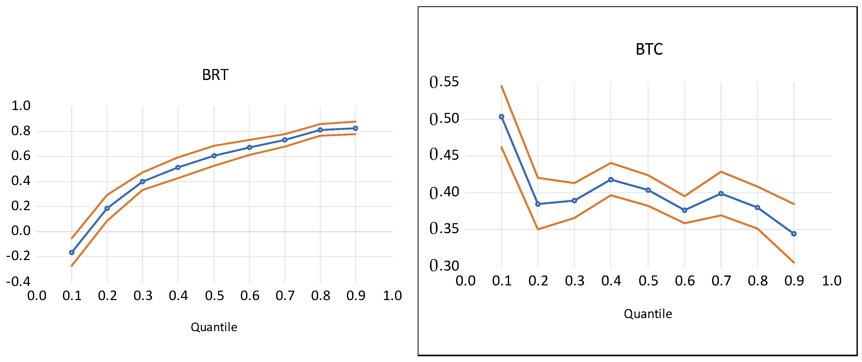
Table 7 and
Figure 4 show that in Equation (12), d
2 is significant when both the OLS method and quantile mediation regression analysis are used. The results demonstrate a significant correlation between BTC as the mediating variable and CO
2 as the response variable, setting up the second stage of the mediating effect of BTC.
After controlling for the mediator variable BTC, using OLS, the explanatory variable BRT is found to be related to the response variable CO2. Equation (12) reveals that d1 is statistically significant, yet smaller than b1 in Equation (10). Since the three steps in Equations (10)–(12) are satisfied, this result indicates the presence of partial mediation.
Using quantile regression mediation analysis (
Table 7) under any CO
2 emission distribution, the response variable CO
2 is significantly influenced by the explanatory variable BRT. Furthermore, the intermediate variable BTC is also significantly related to CO
2. This satisfies all four steps in Equations (10)–(12) and demonstrates the partial mediating effect of BTC. In other words, the outcome indicates that crude oil is a great contributor to CO
2 emissions, with a positive effect observed in all quantiles. Our analysis suggests that through the mediating effect of Bitcoin, crude oil has a negative impact on CO
2 emissions at the 10th percentile, but a more significant positive impact on CO
2 emissions at the upper percentiles compared to the lower percentiles. In addition, our outcome indicates that the connection between crude oil and CO
2 emissions is partly moderated by Bitcoin. Compared to the OLS results, our analysis using quantile regression and mediation techniques provides more exhaustive and encouraging information about the effect of crude oil on CO
2 emissions, and the coefficients obtained are robust evidence.
The x-axis indicates CO2 quantiles and the y-axis indicates BRT and BTC coefficient values. The orange line indicates estimated 95% confidence interval for quantiles.
It is suggested in most of the literature that there is a link between shifts in international economic policy and variations in the returns on Bitcoin investment [
62,
63,
64,
65,
66,
67]. This study uses the EKC concept in nonlinear analysis to observe the relationship among crude oil, Bitcoin, and CO
2 emissions. To the best of our knowledge, this topic has not been explored before.
Table 8 indicates that BRT and BRT
2 are significant predictors of CO
2 emissions at most quantiles, except the 40th percentile, where there is no significant effect. It is noteworthy that according to the definition of Equation (13), α
1 > 0 and α
2 < 0 (BRT
2 coefficients are negative) below the 30th percentile range, indicating a nonlinear inverted U-shaped relationship between crude oil and CO
2 emissions. On the other hand, above the 40th percentile range, α
1 > 0 and α
2 > 0 (BRT
2 coefficients are positive), indicating a nonlinear U-shaped relationship between crude oil and CO
2 emissions. This suggests that CO
2 emissions from crude oil first increase and then decrease at lower percentiles of the CO
2 emission distribution, but decrease and then increase at higher percentiles. This result is consistent with Uchiyama’s argument [
69] that because carbon dioxide is a global pollutant, its effectiveness has not yet been demonstrated within the framework of the Kuznets curve.
Table 9 shows that BTC
2 has a favorable and significant impact on CO
2 emissions across the entire range. According to the definition of Equation (14), β
1 > 0 and β
2 > 0 (BTC
2 coefficients are positive), indicating a nonlinear U-shaped relationship between Bitcoin and CO
2 emissions, but no inverted U-shaped curve exists. This suggests that CO
2 emissions from Bitcoin first decrease and then increase at any CO
2 emission distribution. These results suggest that the energy sources used for Bitcoin mining initially reduce and then increase CO
2 emissions.
4. Discussion
In this study, an innovative approach using quantile-mediated analysis was employed to examine the full range of the impact of crude oil on CO2 emissions through the mediating effect of Bitcoin.
Figure 1 shows a clear breakpoint in CO
2 emissions on 18 March 2020 (i.e., the beginning of the COVID-19 outbreak). The results of the Chow test indicate a structural break in the data for the studied time period, implying a change in the slope trend between the periods before and after that time. With the OLS method, the correct results can only be obtained using data after 18 March 2020. However, the advantage of using quantile regression is that it is not limited by structural changes and can detect the full range of data.
Figure 2 and
Table 6 show the results of quantile regression analysis, indicating that, except for the 10th percentile, crude oil has a negative effect on CO
2 emissions (with a coefficient of −0.032) in the distribution of CO
2 emissions, while it has a positive effect in other distributions. In addition, the positive effect of crude oil on CO
2 emissions suddenly increases after the 40th percentile (with the coefficient rising from 0.52 to 1.164), but it decreases after the 50th percentile (with the coefficient increasing from 1.164 to 1.246). The results indicate that the positive effect of crude oil on CO
2 emissions remains almost constant at the middle and high percentiles, and does not continue to increase.
Figure 3 and
Table 6 show further results of quantile regression analysis, indicating that in the low price range of Bitcoin at the 10th percentile, crude oil has a significant positive effect on Bitcoin (with a coefficient of 1.302), which then decreases suddenly (with the coefficient decreasing from 1.302 to 0.124). As the Bitcoin price distribution moves to the middle and high percentiles, crude oil continues to have a positive impact on Bitcoin prices. At this point, the first stage of the Bitcoin intermediary effect is established.
Figure 4 and
Table 7 show the results of quantile regression analysis after establishing the second stage of the Bitcoin mediation effect. The results indicate that for any CO
2 emission distribution, crude oil has a negative impact on CO
2 emissions except at the 10th percentile (with a coefficient of −0.161), and as the distribution range increases, the positive impact of crude oil on CO
2 emissions continues to increase (with the coefficient increasing from 0.189 to 0.826). However, the impact of Bitcoin on CO
2 emissions shows a gradually decreasing positive influence in a wave-like pattern (with the coefficient fluctuating from 0.503 to 0.344). This shows that, through the partial mediation effect of Bitcoin, the higher the distribution of CO
2 emissions, the higher the positive impact of crude oil.
In addition, we used EKC theory to examine the relationship between crude oil and CO
2 emissions at various percentile ranges of CO
2 emission distribution. The results show that crude oil has an inverted U-shaped relationship with CO
2 emissions below the 30th percentile range and a U-shaped relationship above the 40th percentile range. This is similar to the empirical findings of Rahman and Ahmad [
16] for Pakistan and Alshehry and Belloumi [
13] for Saudi Arabia, both crude oil exporting countries. In addition, the results indicate a nonlinear U-shaped relationship between Bitcoin and CO
2 emissions at any percentile of CO
2 emissions distribution. This is similar to the empirical findings of Truby et al. [
48] regarding the impact of China’s mining ban on the migration of equipment to neighboring countries.
5. Conclusions
In this study, we present a novel approach for analyzing the relationship between crude oil and CO2 emissions and investigate whether Bitcoin volatility plays a mediating role in this relationship. In order to obtain more information efficiently as well as more robust results and to estimate the complete range and distribution of the explanatory variable, we utilized the innovative method of quantile mediation regression. With this method, we explored the direct and indirect impacts of crude oil on CO2 emissions and obtained the following conclusions.
First, crude oil has a direct and an indirect influence on CO2 emissions. This indicates that in the short term, when the price of crude oil increases, CO2 emissions also increase. Our study also reveals a partial mediating impact of Bitcoin volatility in the long term, which results in an indirect positive association between crude oil and CO2 emissions.
Second, crude oil indirectly affects CO
2 emissions through the partial mediation effect of Bitcoin; our findings do not support the presence of an inverted U-shaped curve between Bitcoin and CO
2 emissions, indicating a different interrelationship between the variables. This result indicates that the electricity used for Bitcoin mining initially reduces but then increases CO
2 emissions; however, the positive influence is gradually reduced. This is because the governments of many countries have taken measures in recent years to address the environmental damage caused by Bitcoin mining, including China, Iceland, Canada, and the United States [
48,
70,
71,
72].
Third, the positive impact of crude oil is greater on CO
2 emissions at high quantiles than at low quantiles. The outcome of our study implies that the degree of dependence on crude oil has a direct impact on CO
2 emissions, with higher dependence resulting in a greater effect; it also shows that under the promotion of renewable energy policies in various countries, crude oil usage and CO
2 emissions have not decreased [
11]. Our nonlinear analysis indicates that crude oil exhibits an inverted U-shaped curve for CO
2 emissions below 30% and a U-shaped curve for CO
2 emissions above 30%. This result is consistent with Uchiyama’s argument [
70] that because carbon dioxide is a global pollutant, its effectiveness has not yet been demonstrated within the framework of the Kuznets curve. Our study suggests that a long-term partial adjustment of Bitcoin would have no effect on reducing the effect of crude oil on CO
2 emissions.
Although Bitcoin’s positive impact on CO
2 emissions is gradually decreasing, its intermediary effect has not reduced the impact of crude oil on CO
2 emissions. This indicates that people’s reliance on crude oil has not diminished. In order to achieve the goal of reducing reliance on crude oil to reduce CO
2 emissions, the EU formulated a comprehensive plan for clean energy in 2019, including gradually phasing out gas-powered cars and promoting the use of electric vehicles [
73]. Ilyushin and Fetisov [
74] proposed improving the automatic recovery system for crude oil in order to lower production costs. This study suggests that the government should encourage the use of environmentally friendly and natural materials in the manufacture of everyday products to reduce the demand for crude oil extraction as well as its carbon footprint. Policies should be put in place to support the utilization of more renewable energy sources and the development of infrastructure. Tax reductions or investment incentives should be provided for renewable energy manufacturers to reduce the reliance on crude oil and consequently lower carbon emissions.
This study proposes an innovative method of quantile mediation analysis that integrates the Chow test and EKC. As the applicability of EKC is limited, in future research, we can use this new method in combination with other tests to further investigate the impact of other variables that contribute to climate change and environmental damage and provide references for governments to formulate policies.


