
A Quantitative Risk Assessment Model for Domino Accidents of Hazardous Chemicals Transportation

Abstract
:1. Introduction
2. Materials and Methods
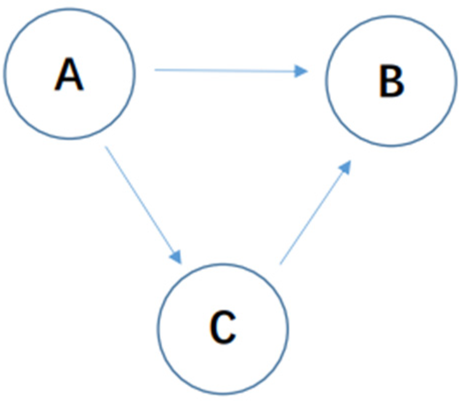
2.1. Dynamic Bayesian Network
- BN describes the relationship between data with the graph method, which has unambiguous semantics and is easy to understand.
- BN allows the learning of causal relationships between variables. It can understand causality in data and learn network structure from the causality.
- BN is good at dealing with missing datasets. The method of BN reflects the probabilistic relationship model between the data in the database and can still establish an accurate model without certain data variables.
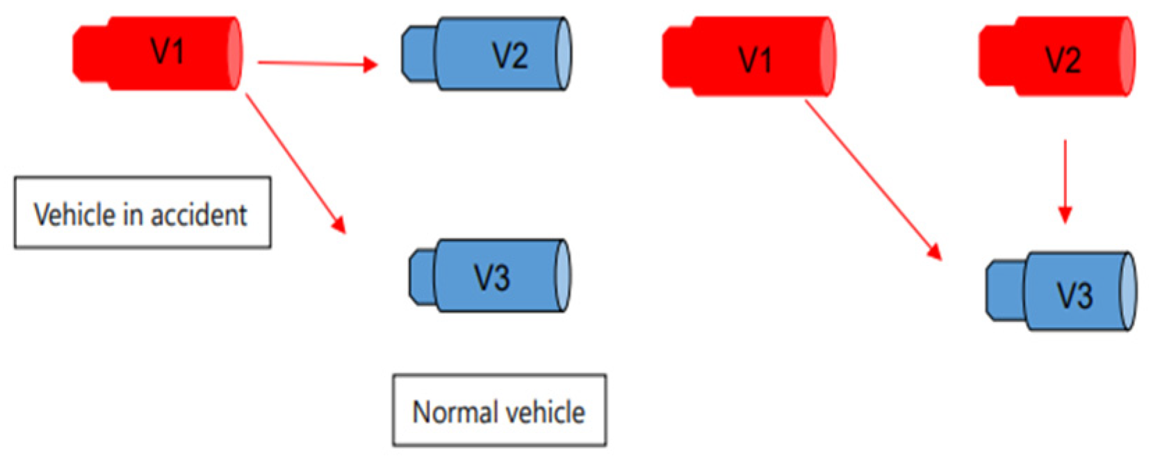
2.2. Domino Effect
2.3. Risk Assessment
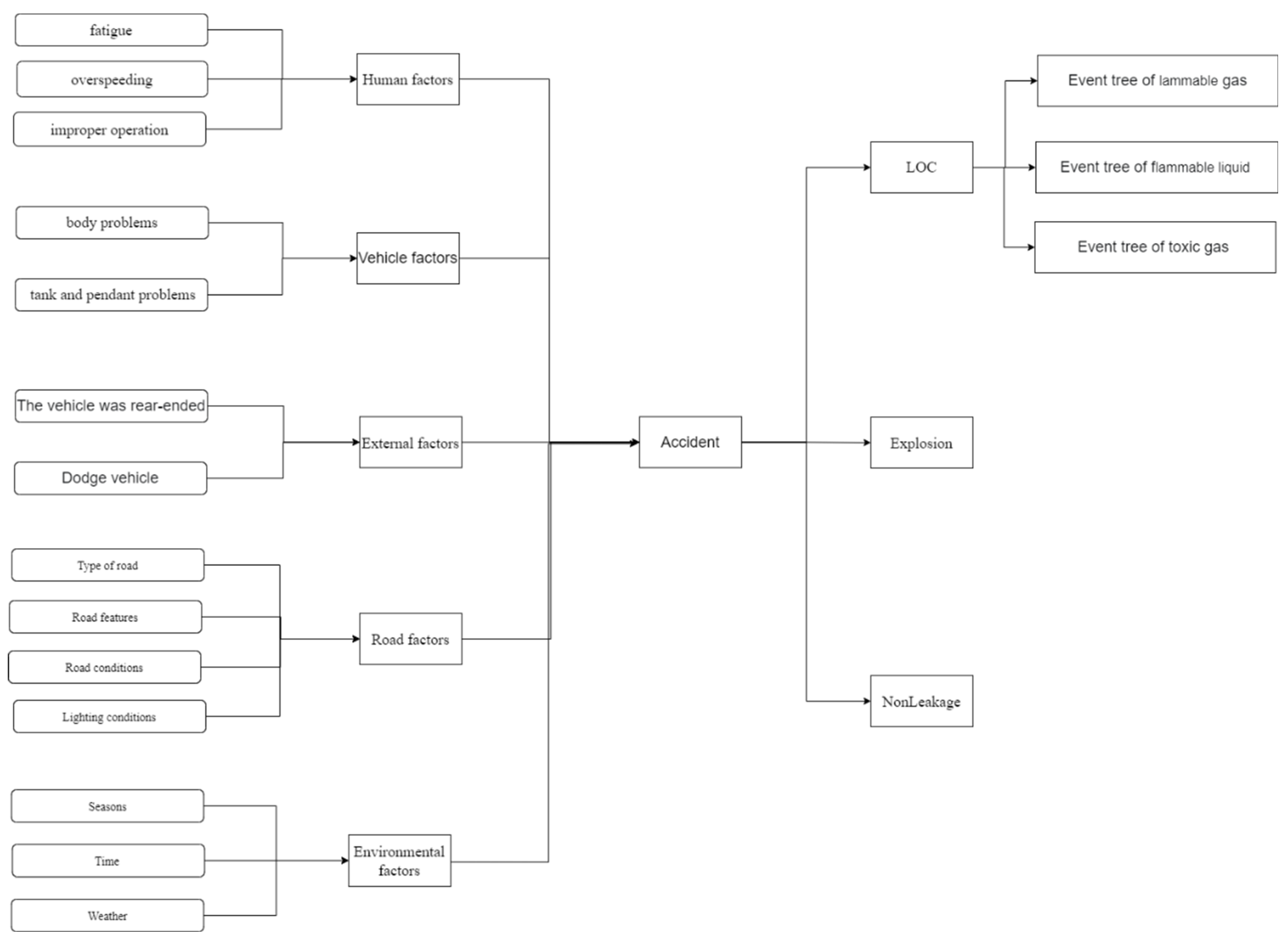
2.3.1. Frequency of Road Transportation Accidents
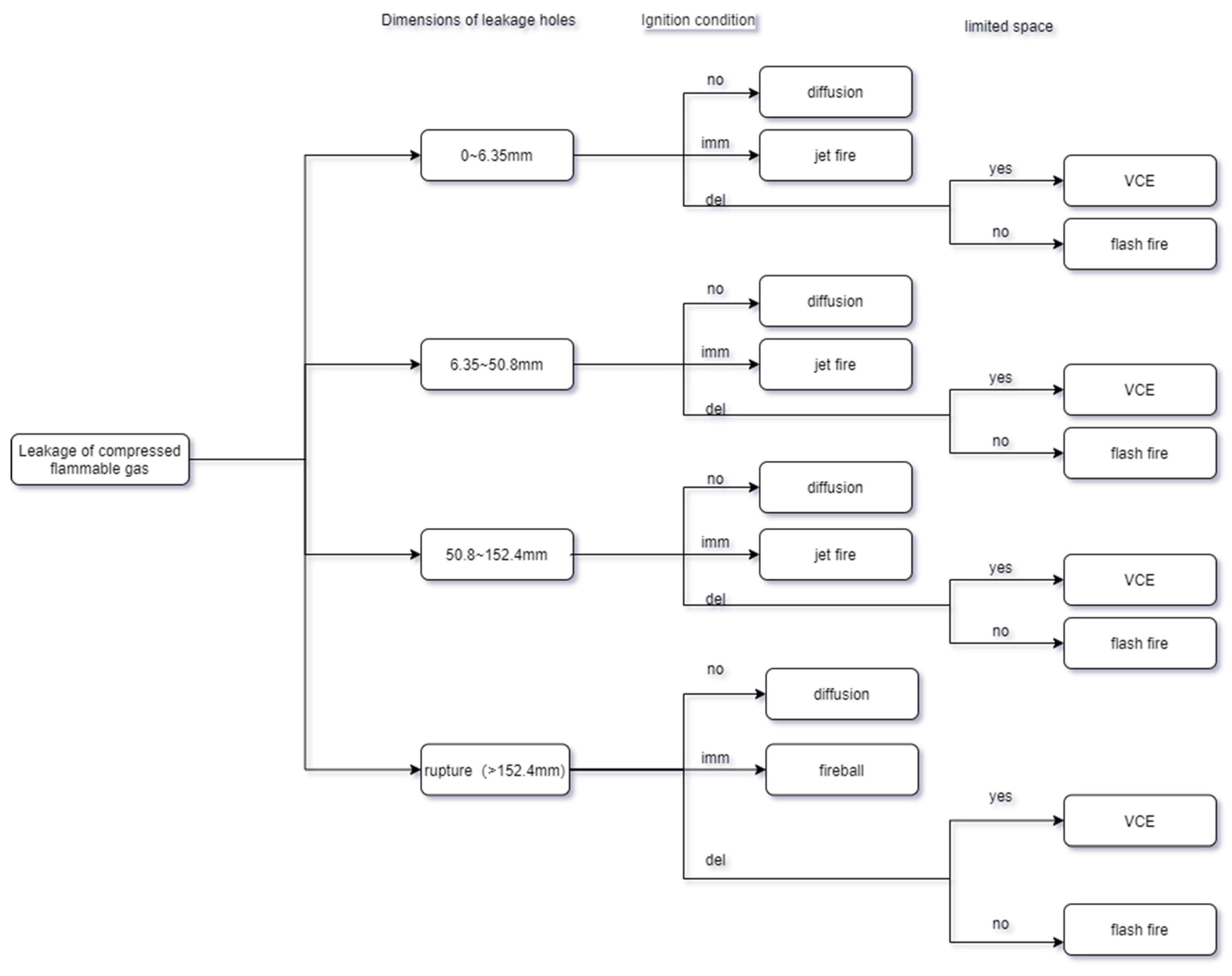
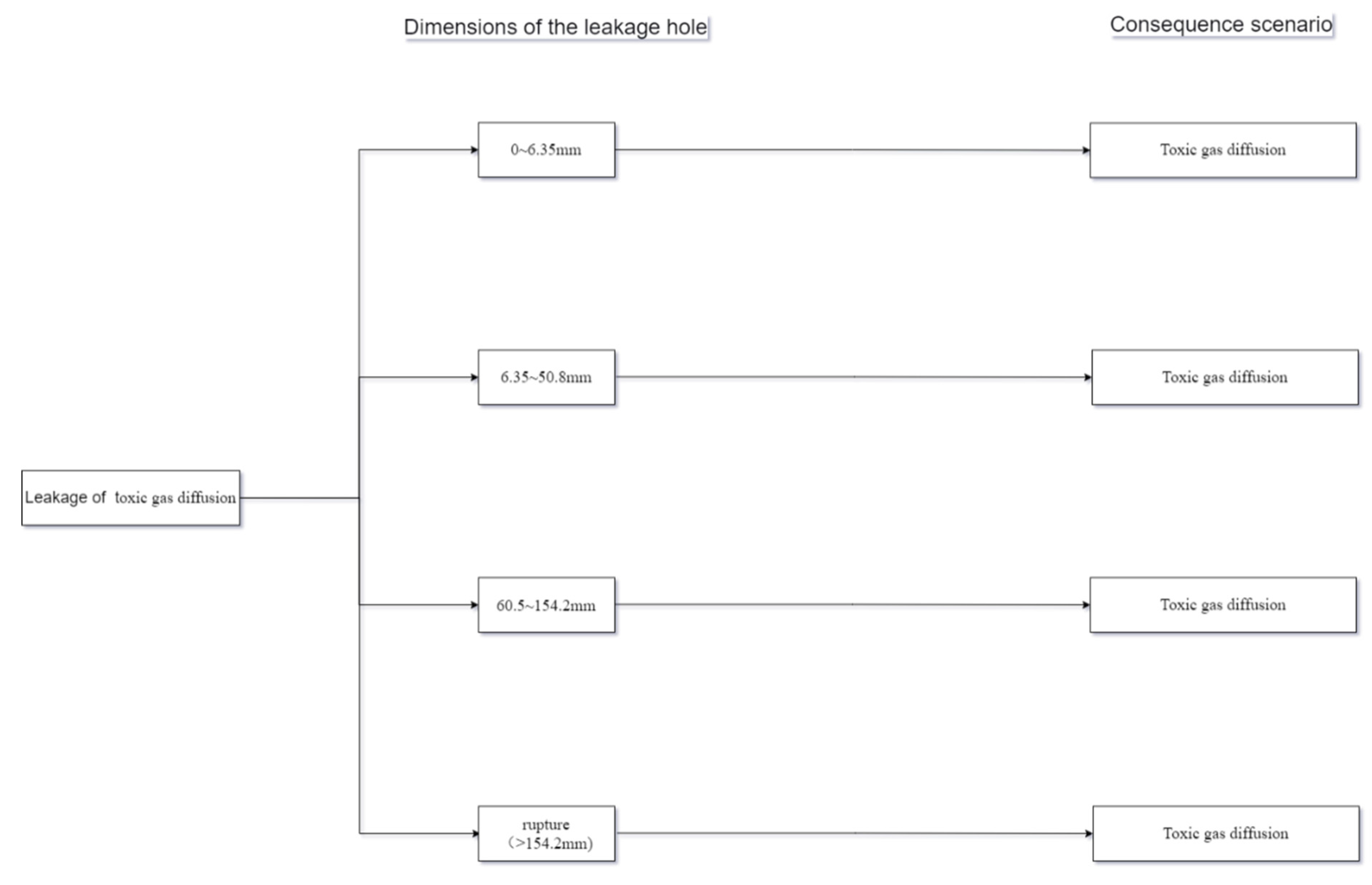
2.3.2. Possibilities of Each Scenario
2.3.3. The Domino Escalation Probability
2.3.4. Casualties of Each Scenario
- Fireball
- Jet fire
- VCE
- Flash Fire
- Diffusion of toxic gas
- Pool fire
2.3.5. Personal Risk and Social Risk
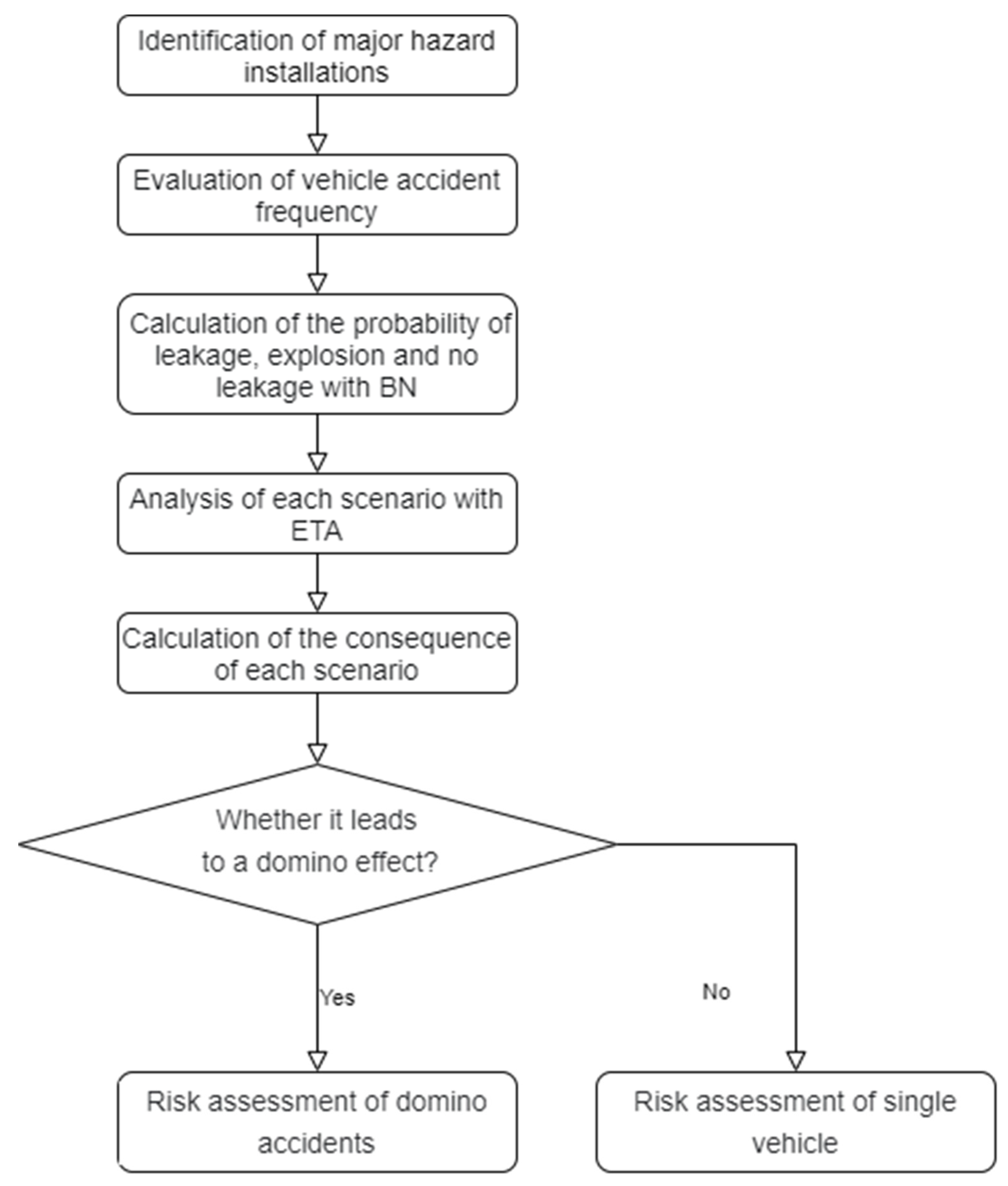
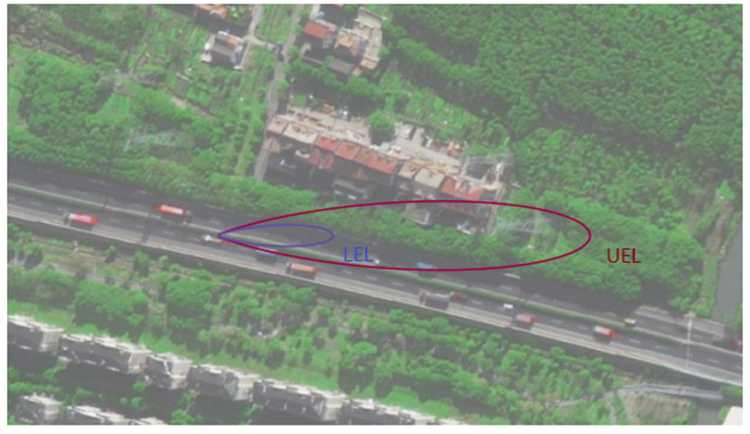
3. Case Study
3.1. Case Analysis Process
3.2. Data
4. Results and Discussion
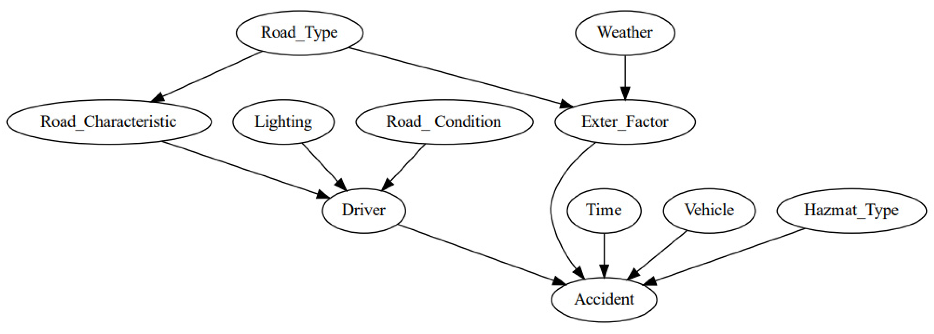
4.1. Structure and Parameters of Dynamic Bayesian Networks
4.2. Risk Analysis of Single Vehicle
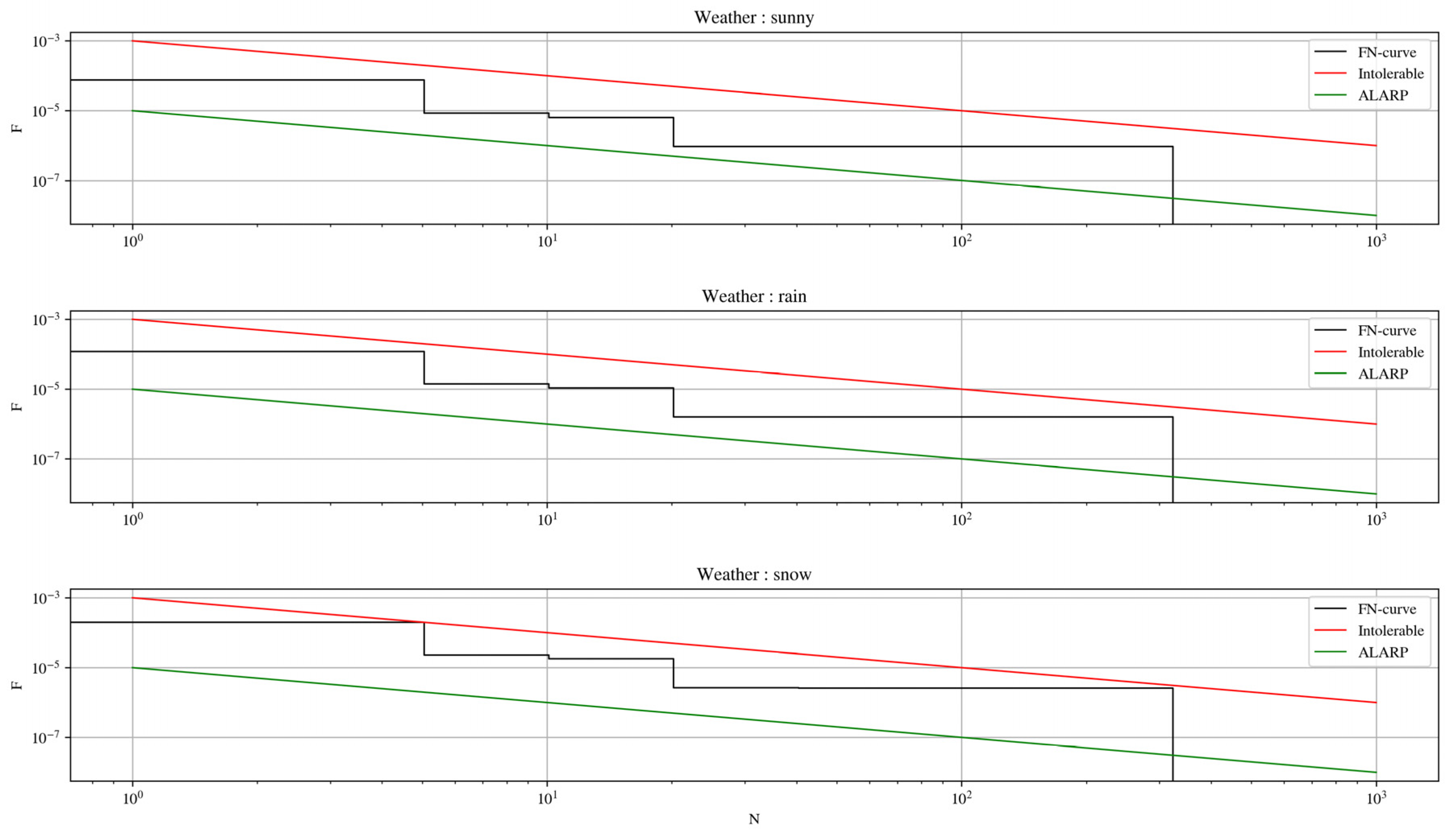
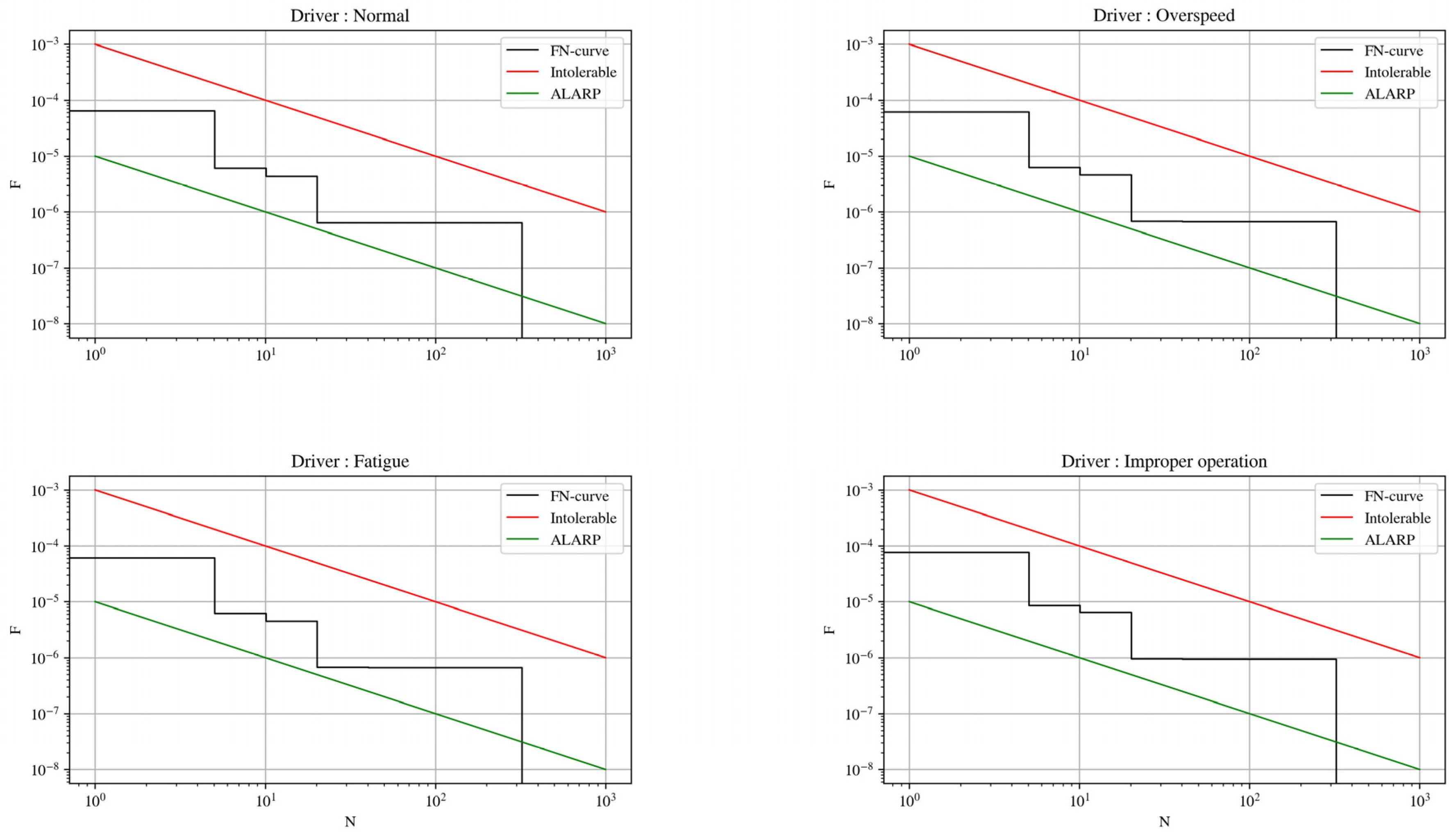
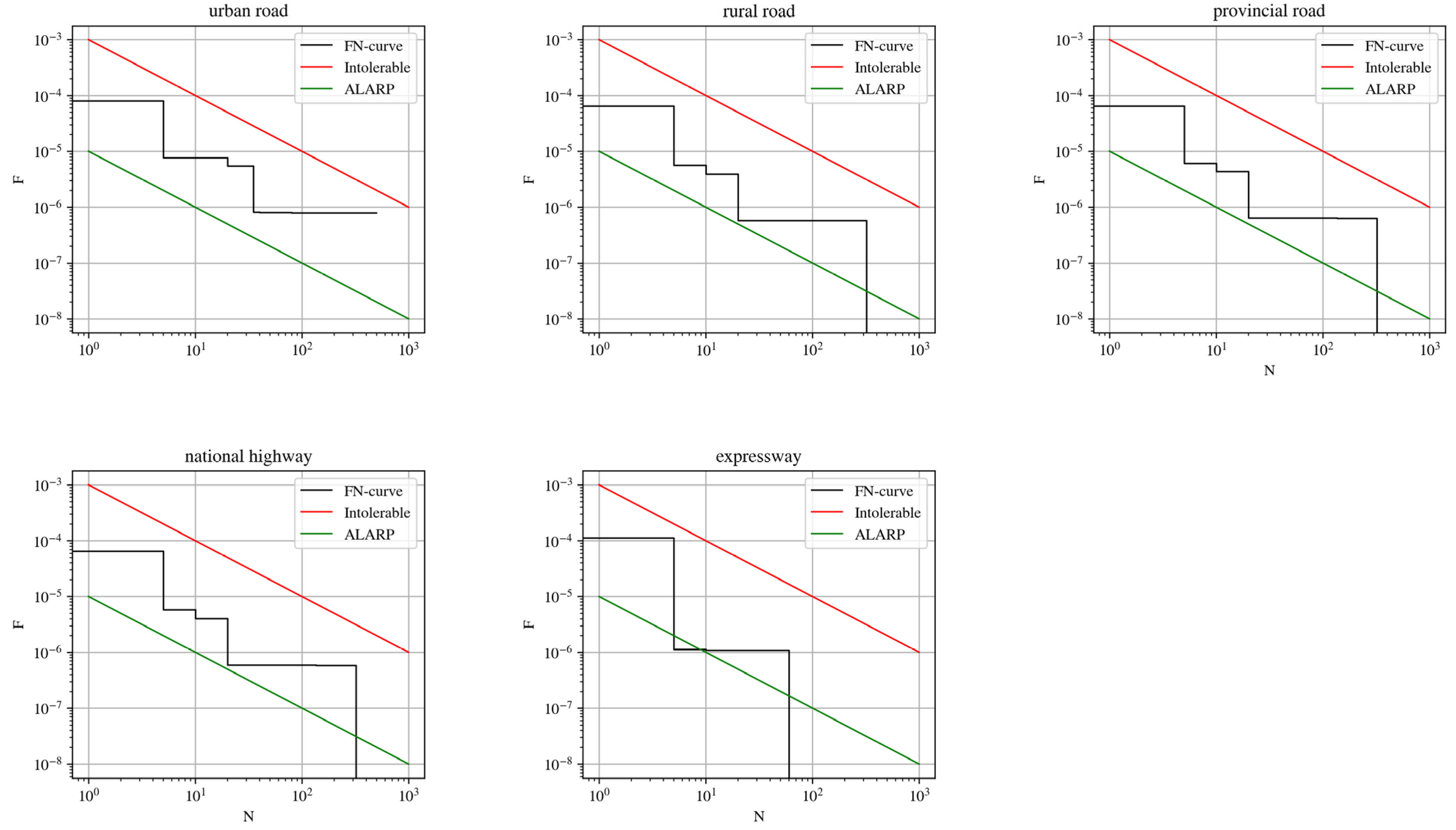
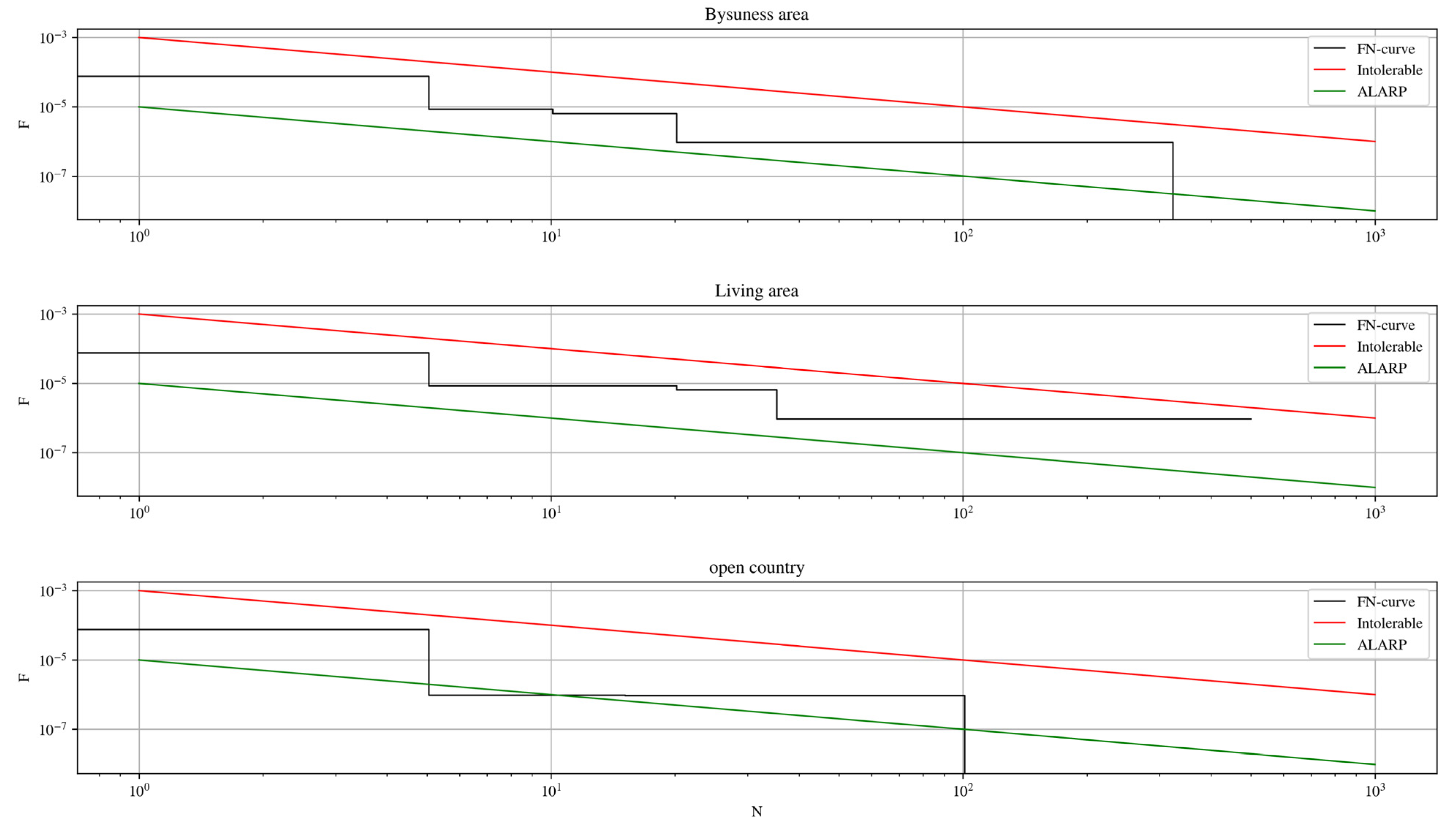
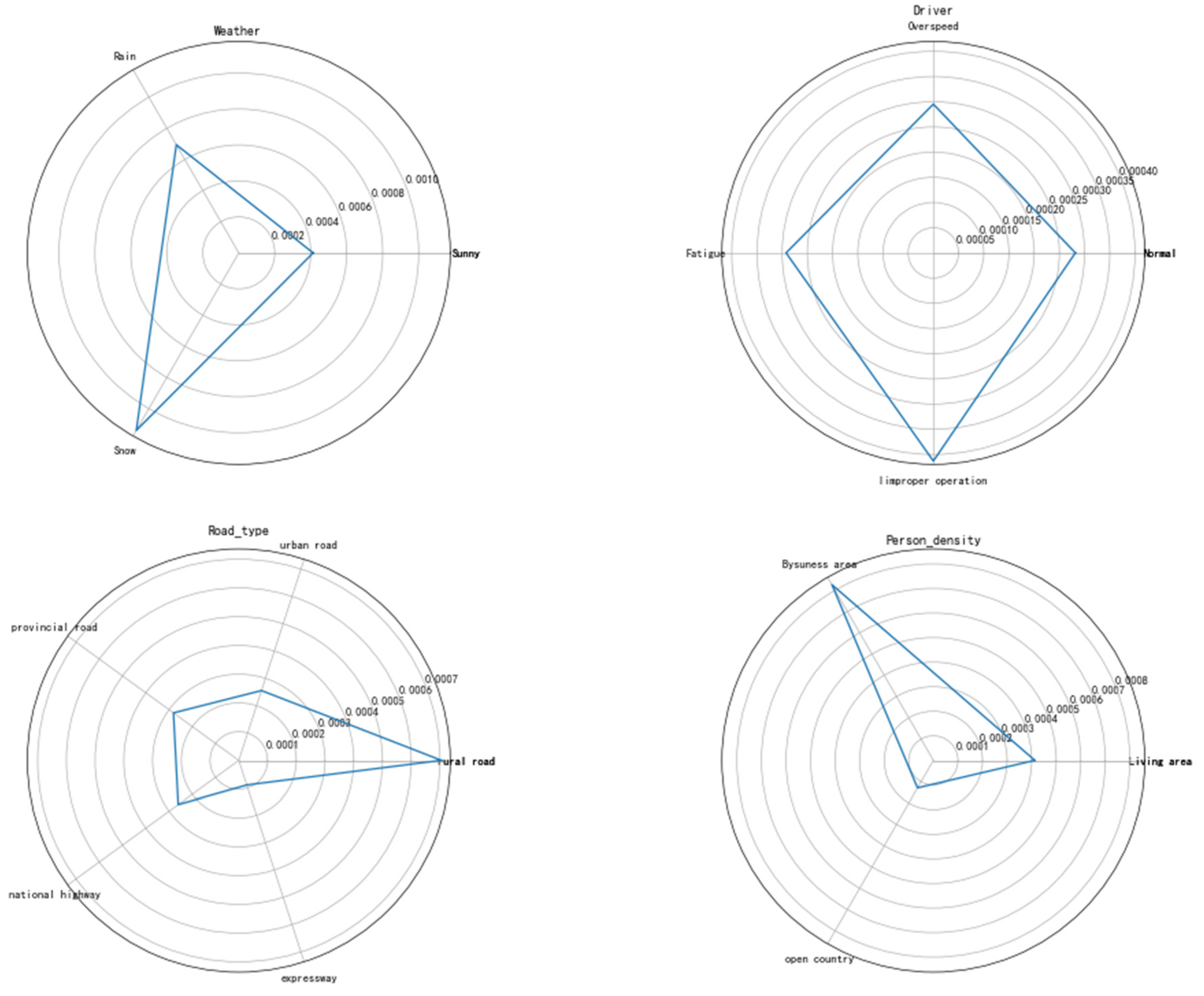
4.3. Analysis of Sensitivity
4.4. Risk Analysis of Multiple Vehicles
5. Conclusions
Author Contributions
Funding
Data Availability Statement
Conflicts of Interest
References
- Ak, R.; Bahrami, M.; Bozkaya, B. A Time-Based Model and GIS Framework for Assessing Hazardous Materials Transportation Risk in Urban Areas. J. Transp. Health 2020, 19, 100943. [Google Scholar] [CrossRef]
- Hong, J.; Tamakloe, R.; Park, D. Application of Association Rules Mining Algorithm for Hazardous Materials Transportation Crashes on Expressway. Accid. Anal. Prev. 2020, 142, 105497. [Google Scholar] [CrossRef] [PubMed]
- Qiao, Y.; Keren, N.; Mannan, M.S. Utilization of Accident Databases and Fuzzy Sets to Estimate Frequency of HazMat Transport Accidents. J. Hazard. Mater. 2009, 167, 374–382. [Google Scholar] [CrossRef] [PubMed]
- Lyu, S.; Zhang, S.; Huang, X.; Peng, S.; Li, J. Investigation and Modeling of the LPG Tank Truck Accident in Wenling, China. Process Saf. Environ. Prot. 2022, 157, 493–508. [Google Scholar] [CrossRef]
- Wiekema, B.J. Vapour cloud explosions—An analysis based on accidents: Part II. J. Hazard. Mater. 1984, 8, 313–329. [Google Scholar] [CrossRef]
- Bagster, D.F.; Pitblado, R. The Estimation of Domino Incident Frequencies—An Approach. Process Saf. Environ. Prot. Trans. Inst. Chem. Eng. Part B 1991, 69, 195–199. [Google Scholar]
- Latha, P.; Gautam, G.; Raghavan, K.V. Strategies for the quantification of thermally initiated cascade effects. J. Loss Prev. Process Ind. 1992, 5, 18–27. [Google Scholar] [CrossRef]
- Pettitt, G.N.; Schumacher, R.R.; Seeley, L.A. Evaluating the probability of major hazardous incidents as a result of escalation events. J. Loss Prev. Process Ind. 1993, 6, 37–46. [Google Scholar] [CrossRef]
- Pompone, E.C.; Neto, G.C.; de Oliveira, N.G.C. A Survey on Accidents in the Road Transportation of Hazardous Materials in São Paulo, Brazil, from 1983 to 2015. Transp. Res. Rec. 2019, 2673, 285–293. [Google Scholar] [CrossRef]
- Erkut, E.; Alp, O. Designing a Road Network for Hazardous Materials Shipments. Comput. Oper. Res. 2007, 34, 1389–1405. [Google Scholar] [CrossRef]
- Fabiano, B.; Currò, F.; Palazzi, E.; Pastorino, R. A Framework for Risk Assessment and Decision-Making Strategies in Dangerous Good Transportation. J. Hazard. Mater. 2002, 93, 1–15. [Google Scholar] [CrossRef] [PubMed]
- Landucci, G.; Antonioni, G.; Tugnoli, A.; Bonvicini, S.; Molag, M.; Cozzani, V. HazMat Transportation Risk Assessment: A Revisitation in the Perspective of the Viareggio LPG Accident. J. Loss Prev. Process Ind. 2017, 49, 36–46. [Google Scholar] [CrossRef]
- Weng, J.; Gan, X.; Zhang, Z. A Quantitative Risk Assessment Model for Evaluating Hazmat Transportation Accident Risk. Saf. Sci. 2021, 137, 105198. [Google Scholar] [CrossRef]
- Tao, D.; Zhang, R.; Qu, X. The Role of Personality Traits and Driving Experience in Self-Reported Risky Driving Behaviors and Accident Risk among Chinese Drivers. Accid. Anal. Prev. 2017, 99, 228–235. [Google Scholar] [CrossRef] [PubMed]
- Benekos, I.; Diamantidis, D. On Risk Assessment and Risk Acceptance of Dangerous Goods Transportation through Road Tunnels in Greece. Saf. Sci. 2017, 91, 1–10. [Google Scholar] [CrossRef]
- Bonvicini, S.; Leonelli, P.; Spadoni, G. Risk Analysis of Hazardous Materials Transportation: Evaluating Uncertainty by Means of Fuzzy Logic. J. Hazard. Mater. 1998, 62, 59–74. [Google Scholar] [CrossRef]
- Reniers, G.L.L.; Jongh, K.D.; Gorrens, B.; Lauwers, D.; Leest, M.V.; Witlox, F. Transportation Risk ANalysis Tool for Hazardous Substances (TRANS)—A User-Friendly, Semi-Quantitative Multi-Mode Hazmat Transport Route Safety Risk Estimation Methodology for Flanders. Transp. Res. Part D Transp. Environ. 2010, 15, 489–496. [Google Scholar] [CrossRef]
- Matias, J.; Taboada, J.; Ordonez, C.; Nieto, P. Machine Learning Techniques Applied to the Determination of Road Suitability for the Transportation of Dangerous Substances. J. Hazard. Mater. 2007, 147, 60–66. [Google Scholar] [CrossRef]
- Li, J.; Reniers, G.; Cozzani, V.; Khan, F. A bibliometric analysis of peer-reviewed publications on domino effects in the process industry. J. Loss Prev. Process Ind. 2017, 49, 103–110. [Google Scholar] [CrossRef]
- Khakzad, N.; Khan, F.; Amyotte, P.; Cozzani, V. Domino Effect Analysis Using Bayesian Networks. Risk Anal. 2013, 33, 292–306. [Google Scholar] [CrossRef]
- Zarei, E.; Gholamizadeh, K.; Khan, F.; Khakzad, N. A dynamic domino effect risk analysis model for rail transport of hazardous material. J. Loss Prev. Process Ind. 2022, 74, 104666. [Google Scholar] [CrossRef]
- Yang, J.; Li, F.; Zhou, J.; Zhang, L.; Huang, L.; Bi, J. A Survey on Hazardous Materials Accidents during Road Transport in China from 2000 to 2008. J. Hazard. Mater. 2010, 184, 647–653. [Google Scholar] [CrossRef] [PubMed]
- Li, R.; Leung, Y. Multi-Objective Route Planning for Dangerous Goods Using Compromise Programming. J. Geogr. Syst. 2011, 13, 249–271. [Google Scholar] [CrossRef]
- Weber, P.; Medina-Oliva, G.; Simon, C.; Iung, B. Overview on Bayesian Networks Applications for Dependability, Risk Analysis and Maintenance Areas. Eng. Appl. Artif. Intell. 2012, 25, 671–682. [Google Scholar] [CrossRef]
- Ma, T.; Wang, Z.; Yang, J.; Huang, C.; Liu, L.; Chen, X. Real-Time Risk Assessment Model for Hazmat Release Accident Involving Tank Truck. J. Loss Prev. Process Ind. 2022, 77, 104759. [Google Scholar] [CrossRef]
- Huang, W.; Chen, X.; Qin, Y. A simulation method for the dynamic evolution of domino accidents in chemical industrial Parks. Process Saf. Environ. Prot. 2022, 168, 96–113. [Google Scholar] [CrossRef]
- Caliendo, C.; De Guglielmo, M.L. Quantitative Risk Analysis on the Transport of Dangerous Goods Through a Bi-Directional Road Tunnel: Quantitative Risk Analysis on the Transport of Dangerous Goods. Risk Anal. 2017, 37, 116–129. [Google Scholar] [CrossRef]
- Chakrabarti, U.K.; Parikh, J.K. Risk-Based Route Evaluation against Country-Specific Criteria of Risk Tolerability for Hazmat Transportation through Indian State Highways. J. Loss Prev. Process Ind. 2013, 26, 723–736. [Google Scholar] [CrossRef]
- Vidmar, P.; Perkovič, M. Safety Assessment of Crude Oil Tankers. Saf. Sci. 2018, 105, 178–191. [Google Scholar] [CrossRef]
- Zhang, Y.; Luo, Y.; Pei, J.; Hao, Y.; Zeng, Z.; Yang, Y. The Establishment of Gas Accident Risk Tolerability Criteria Based on F–N Curve in China. Nat. Hazards 2015, 79, 263–276. [Google Scholar] [CrossRef]
- Qiu, S.; Sacile, R.; Sallak, M.; Schön, W. On the Application of Valuation-Based Systems in the Assessment of the Probability Bounds of Hazardous Material Transportation Accidents Occurrence. Saf. Sci. 2015, 72, 83–96. [Google Scholar] [CrossRef]
- Zhang, J.; Hodgson, J.; Erkut, E. Using GIS to Assess the Risks of Hazardous Materials Transport in Networks. Eur. J. Oper. Res. 2000, 121, 316–329. [Google Scholar] [CrossRef]
- Heckerman, D. Bayesian Graphical Models and Networks. In International Encyclopedia of the Social & Behavioral Sciences, 2nd ed.; Wright, J.D., Ed.; Elsevier: Oxford, UK, 2015; pp. 363–367. [Google Scholar] [CrossRef]
- Xu, Y.; Reniers, G.; Yang, M.; Yuan, S.; Chen, C. Uncertainties and their treatment in the quantitative risk assessment of domino effects: Classification and review. Process Saf. Environ. Prot. 2023, 172, 971–985. [Google Scholar] [CrossRef]
- Cozzani, V.; Salzano, E. The quantitative assessment of domino effects caused by overpressure: Part I. Probit models. J. Hazard. Mater. 2004, 107, 67–80. [Google Scholar] [CrossRef]
- Shen, Z.; Lang, J.; Li, M.; Mao, S.; Hu, F.; Xuan, B. Impact of inlet boundary number and locations on gas diffusion and flow in a typical chemical industrial park near uneven Terrain. Process Saf. Environ. Prot. 2022, 159, 281–293. [Google Scholar] [CrossRef]
- Feng, J.R.; Gai, W.; Yan, Y. Emergency evacuation risk assessment and mitigation strategy for a toxic gas leak in an underground space: The case of a subway station in Guangzhou, China. Saf. Sci. 2021, 134, 105039. [Google Scholar] [CrossRef]
- Holeczek, N. Hazardous materials truck transportation problems: A classification and state of the art literature review. Transp. Res. Part D Transp. Environ. 2019, 69, 305–328. [Google Scholar] [CrossRef]
- Liu, Y.; Fan, L.; Li, X.; Shi, S.; Lu, Y. Trends of hazardous material accidents (HMAs) during highway transportation from 2013 to 2018 in China. J. Loss Prev. Process Ind. 2020, 66, 104150. [Google Scholar] [CrossRef]
- Li, Y.; Wang, Y.; Lai, Y.; Shuai, J.; Zhang, L. Monte Carlo-based quantitative risk assessment of parking areas for vehicles carrying hazardous chemicals. Reliab. Eng. Syst. Saf. 2023, 231, 109010. [Google Scholar] [CrossRef]


| Meteorological Conditions | H1 | Traffic Characteristics (vehicles/h) | H2 |
|---|---|---|---|
| Sunny | 1.0 | ≤500 | 0.8 |
| Rain/fog | 1.5 | 500 < Traffic flow < 1250 | 1.0 |
| Snow/ice | 2.5 | ≥1250 | 1.4 |
| Accident Information | Specific Content |
|---|---|
| Human factors | Normal, fatigue, speeding, improper operation |
| External factors | None, being rear-ended, dodging vehicles |
| Vehicle factors | Vehicle type (tanker, trailer, van, other) Vehicle problems (normal, body problems, tank and pendant problems) |
| Environmental factors | Seasons (spring, summer, autumn, winter) Time (morning, afternoon, evening, early morning) Weather (sunny, cloudy, rainy, overcast, snowy, foggy) |
| Road factors | Type of road (expressway, national highway, provincial road, urban road, rural road) Feature of road (no distinguishing features, curves, junctions, tunnels, ramps) Road conditions (dry, wet) Lighting conditions (daytime, no lighting at night, illumination at night) |
| Consequences of the accident | No leakage, leakage of hazardous materials, explosion. |
| Size of Leakage Hole | Percentage of Leakage Hole |
|---|---|
| 0~1/4 in. | 82.41% |
| 1/4~2 in. | 14.51% |
| 2~6 in. | 2.9% |
| Greater than 6 in. | 0.18% |
| Category | Leaked Scene | Probability of Immediate Ignition |
|---|---|---|
| 0 | Continuous leak | 0.1 |
| Instantaneous leakage | 0.4 | |
| 1 | / | 0.065 |
| 2 | / | 0.01 |
| 3,4 | / | 0 |
| Ignition Source | Efficiency |
|---|---|
| Flame | 1.0 |
| Vehicle | 0.4 |
| Person | 0.01 |
| Vector of Escalation | Type of Container | Mathematical Model of Damage Probability |
|---|---|---|
| Thermal radiation | Atmospheric vessel | |
| Thermal radiation | Pressure vessels | |
| Overpressure | Atmospheric vessel | |
| Overpressure | Pressure vessels |
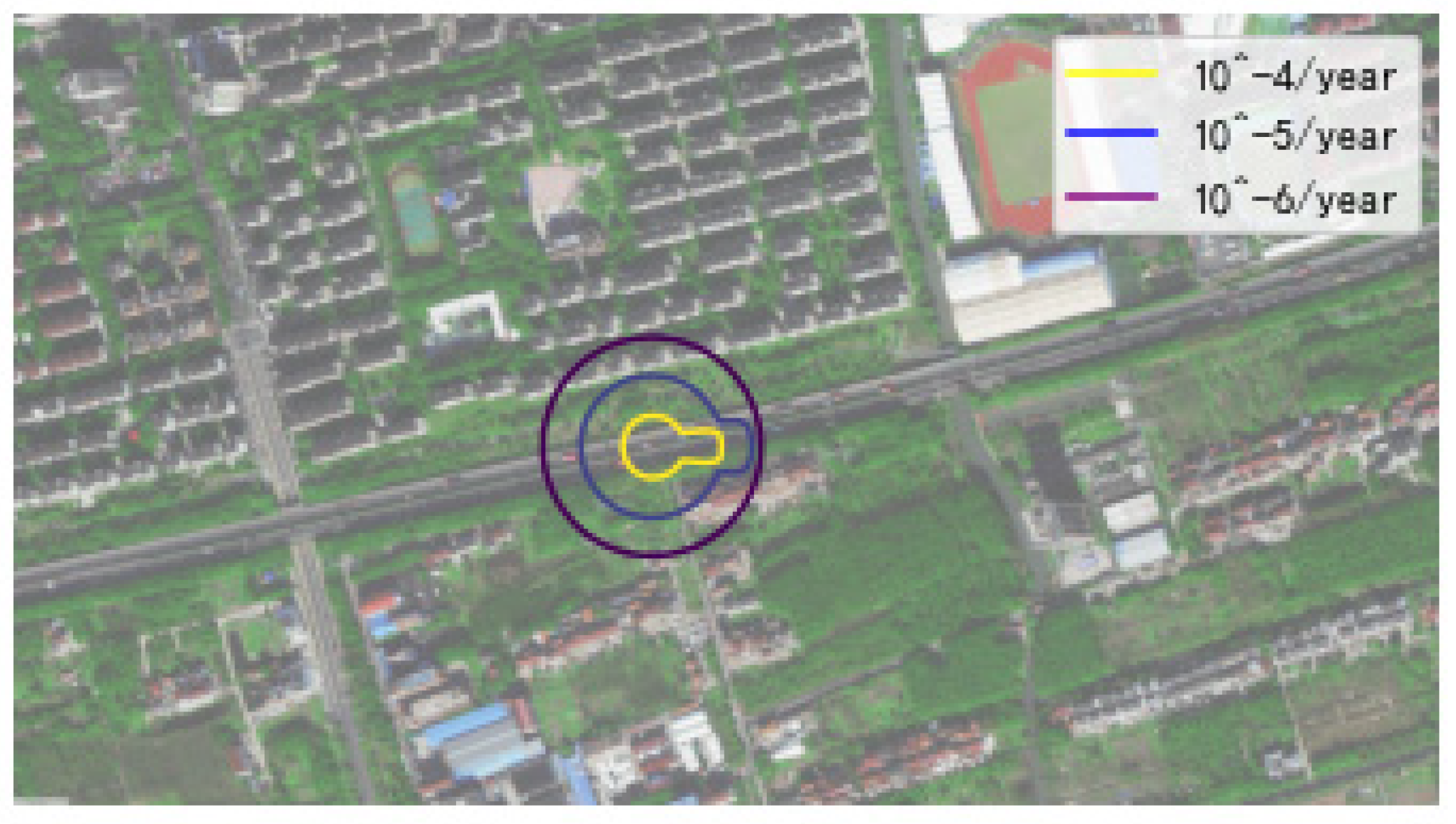
| Protection Target | Personal Acceptable Risk Criteria (Probability Value) | ||
|---|---|---|---|
| New Equipment (Per Year) | Equipment in Service (Per Year) | ||
| China | Low-density places (number of people < 30) | 1 × 10⁻⁵ | 3 × 10⁻⁵ |
| Residential high-density places (30 ≤ number of people < 100) High-density public gathering places (30 ≤ number of people < 100): | 3 × 10⁻⁶ | 1 × 10⁻⁵ | |
| Highly sensitive places: schools, hospitals, nursing homes, etc. Important targets: military restricted areas, cultural protection units. | 3 × 10⁻⁷ | 1 × 10⁻⁶ | |
| Britain | Acceptable casualty standards for the public and workers | 1 × 10⁻⁶ | |
| Unacceptable casualty standards for the public and workers | 1 × 10⁻⁴ | ||
| Parameter | Value |
|---|---|
| Driver status of vehicle I | Normal |
| Hazardous substances in vehicle I | Ammonia |
| Vehicle status of vehicle I | Normal |
| Storage pressure of vehicle I | 100 kPa |
| Quality of goods in vehicle I | kg |
| Tank size of vehicle I | 1 m (radius), 3 m (length) |
| Storage temperature of vehicle I | −40 °C |
| Hazardous substances in vehicle II | 1–3 butadiene |
| Driver status of vehicle II | Normal |
| Vehicle status of vehicle II | Normal |
| Storage pressure of vehicle II | 500 kPa |
| Storage temperature of vehicle II | 10 °C |
| Quality of goods in vehicle II | 17,500 kg |
| Tank size of vehicle II | 1 m (radius), 5 m (length) |
| The explosive limit of 1,3_butadiene | 1.1%~16.1% |
| The density of 1,3_butadiene | |
| The melting point of 1,3_butadiene | −108.9 °C |
| Molecular weight of 1,3_butadiene | 54.09 |
| Heat of combustion of butadiene | 2541.0 KJ/mol |
| Molecular weight of liquid ammonia | 17.04 |
| The density of liquid ammonia(25 ℃) | |
| Materials toxicity constant ammonia | a = −15.6, b = 1, n = 2 |
| Atmospheric stability | B |
| Traffic characteristics | 485 vehicles/h |
| Population density | 1600 / |
| Relative humidity | 30% |
| Wind speed | 1.5 m/s |
| Temperature | 25 °C |
| Road type | Urban road |
| Weather | Sunny |
| Timing | Daytime |
| VAR | per (vehicle kilometers) |
| L | km |
| Driver | Vehicle | External Factors | Type of Road | Light | Weather | Accident |
|---|---|---|---|---|---|---|
| Normal | Normal | None | National highway | Day | Foggy | Leakage |
| Improper operation | Normal | None | Provincial road | Night | Sunny | Leakage |
| Speeding | Normal | None | National highway | Day | Runny | Leakage |
| Normal | Normal | None | Backroad | Day | Sunny | No leakage |
| Improper operation | Normal | None | Backroad | Day | Sunny | Leakage |
| Improper operation | Normal | None | Rural road | Day | Rainy | Explosion |
| Node Name | Value Set |
|---|---|
| Driver | Normal (0) fatigue (1), over speeding (2), improper operation (3) |
| Vehicle | Normal (0), body problems (1), tank problems (2) |
| Timing | Day (0), afternoon (1), night (2), midnight (3) |
| Light | Day (0), night with lights (1), night without lights (2) |
| External factor | Normal (0), the vehicle was rear-ended (1), overtake (1) |
| Weather | Sunny (0), cloudy (1), rainy (2), snowy (3), foggy (4) |
| Type of Road | Rural road (0), road (1), national highway (2), Provincial road (3), expressway (4) |
| Characteristic of road | Normal (0), curve (1), junction (2), tunnel (3) ramp (4) |
| Type of Hazmat | Flammable (0), explosive (1), toxic (2) |
| Driver | Vehicle | External Factors | Type of Road | Light | Weather | Actual Result | Predicted Result |
|---|---|---|---|---|---|---|---|
| Normal | Normal | None | National highway | Day | Foggy | Leakage | Leakage |
| Improper operation | Normal | None | Provincial road | Night | Sunny | Leakage | Leakage |
| Speeding | Normal | None | National highway | Day | Runny | Leakage | No leakage |
| Normal | Normal | None | Backroad | Day | Sunny | No leakage | No leakage |
| Improper operation | Normal | None | Backroad | Day | Sunny | Leakage | Leakage |
| Improper operation | Normal | Overtake | Rural road | Day | Rainy | Explosion | Explosion |
| Accident Type | Probability |
|---|---|
| LOC | 0.6872 |
| No leaks | 0.2895 |
| Explosion | 0.0233 |
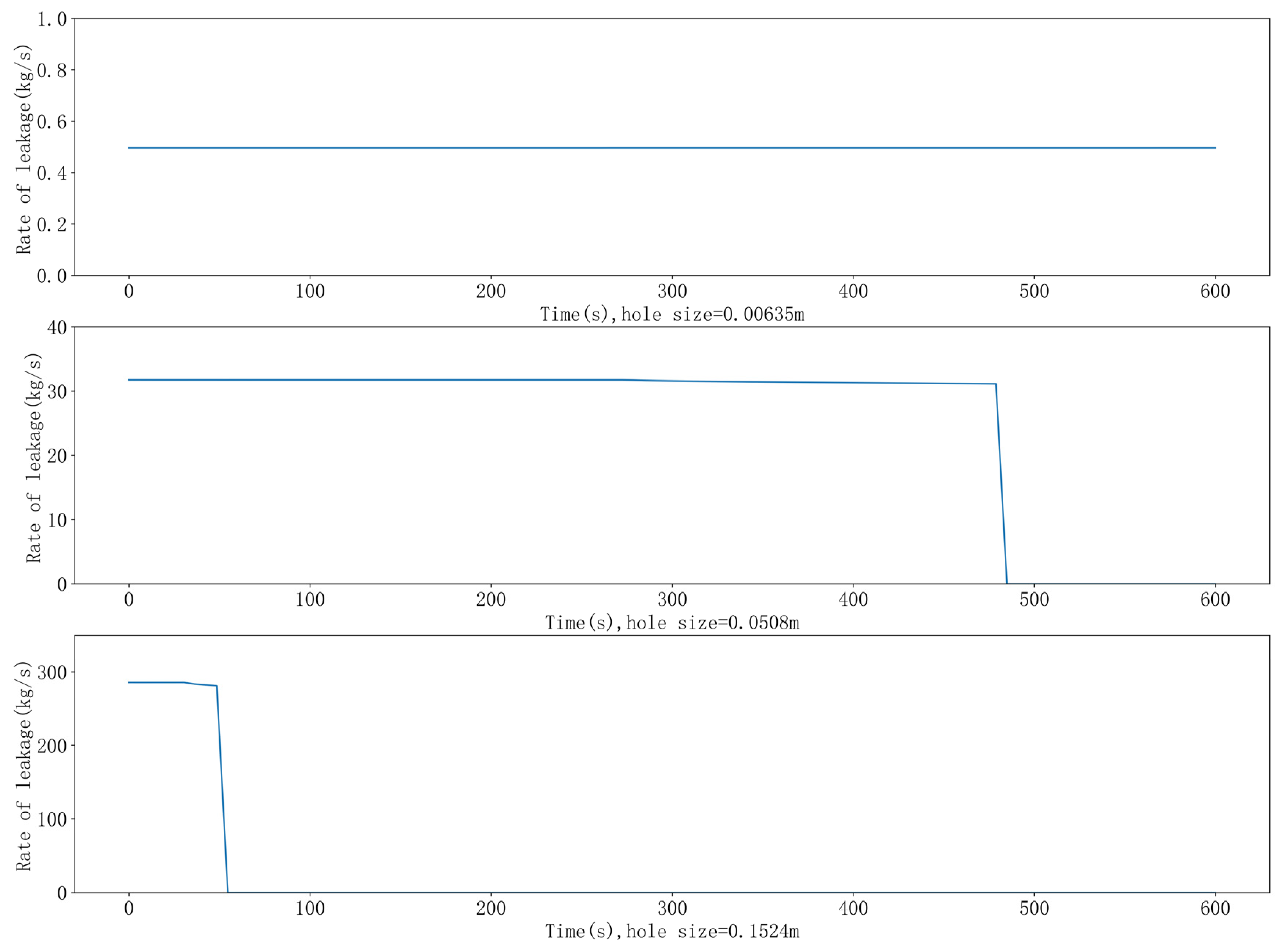
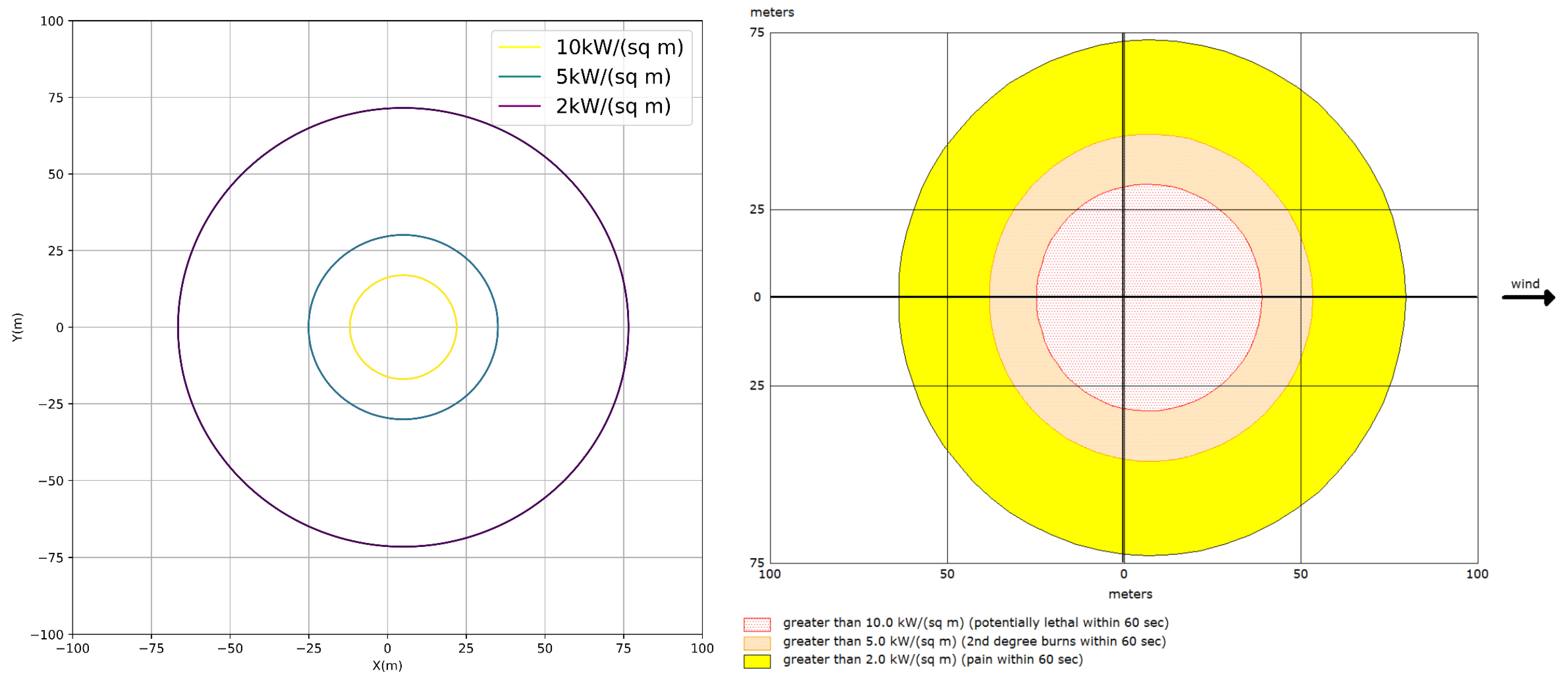
| Accident Scenario | Frequency | Thermal Radiation/ Overpressure Value | The Probability of Escalation | PLL without Domino | PLL with Domino | Hole Size |
|---|---|---|---|---|---|---|
| Fireball | 7.38 × 10⁻⁶ | 38.2 | 0.23 | 16 | 32 | rupture |
| VCE | 9.43 × 10⁻⁷ | 201.08 Kpa | 0.99 | 318 | 321 | rupture |
| Jet fire | 5.72 × 10⁻⁵ | 1.05 | 0.005 | 1 | 19 | 0.00635 m |
| VCE | 2.59 × 10⁻⁸ | 2.98 Kpa | 4.61 × 10⁻⁶ | 1 | 20 | 0.00635 m |
| Flash fire | 3.29 × 10⁻⁸ | / | 0 | 1 | 1 | 0.00635 m |
| Jet fire | 1.00 × 10⁻⁵ | 14.80 | 0.03 | 1 | 19 | 0.0508 m |
| VCE | 1.00 × 10⁻⁵ | 83 Kpa | 0.99 | 32 | 45 | 0.0508 m |
| Flash fire | 5.23 × 10⁻⁶ | / | 0 | 4 | 4 | 0.0508 m |
| Jet fire | 2.01 × 10⁻⁶ | 14.80 | 0.03 | 1 | 19 | 0.1524 m |
| VCE | 9.12 × 10⁻¹⁰ | 12.49 Kpa | 0.17 | 135 | 137 | 0.1524 m |
| Flash fire | 7.34 × 10⁻¹⁰ | / | 0 | 9 | 9 | 0.1524 m |
Disclaimer/Publisher’s Note: The statements, opinions and data contained in all publications are solely those of the individual author(s) and contributor(s) and not of MDPI and/or the editor(s). MDPI and/or the editor(s) disclaim responsibility for any injury to people or property resulting from any ideas, methods, instructions or products referred to in the content. |
© 2023 by the authors. Licensee MDPI, Basel, Switzerland. This article is an open access article distributed under the terms and conditions of the Creative Commons Attribution (CC BY) license (https://creativecommons.org/licenses/by/4.0/).
Share and Cite
Cheng, J.; Wang, B.; Cao, C.; Lang, Z. A Quantitative Risk Assessment Model for Domino Accidents of Hazardous Chemicals Transportation. Processes 2023, 11, 1442. https://doi.org/10.3390/pr11051442
Cheng J, Wang B, Cao C, Lang Z. A Quantitative Risk Assessment Model for Domino Accidents of Hazardous Chemicals Transportation. Processes. 2023; 11(5):1442. https://doi.org/10.3390/pr11051442
Chicago/Turabian StyleCheng, Jinhua, Bing Wang, Chenxi Cao, and Ziqiang Lang. 2023. "A Quantitative Risk Assessment Model for Domino Accidents of Hazardous Chemicals Transportation" Processes 11, no. 5: 1442. https://doi.org/10.3390/pr11051442