Artificial Intelligent Power Forecasting for Wind Farm Based on Multi-Source Data Fusion

Abstract

Wind power forecasting is a typical high-dimensional and multi-step time series prediction problem. Data-driven prediction methods using machine learning show advantages over traditional physical or statistical methods, especially for wind farms with complex meteorological conditions. Thus, effective use of different data sources and data types will help improve power forecasting accuracy. In this paper, a multi-source data fusion method is proposed, which integrates the static information of the wind turbine with observational and forecasting meteorological information together to further improve the power forecasting accuracy. Firstly, the characteristics of each time step are re-characterized by using the self-attention mechanism to integrate the global information of multi-source data, and the Res-CNN network is used to fuse multi-source data to improve the prediction ability of input variables. Secondly, static variable encoding and feature selection are carried out, and the time-varying variables are combined with static variables for collaborative feature selection, so as to effectively eliminate redundant information. A forecasting model based on the Encoder–Decoder framework is constructed with LSTM as the basic unit, and the Add&Norm mechanism is introduced to further enhance the input variable information. In addition, the self-attention mechanism is used to integrate the global time information of the decoded results, and the Time Distributed mechanism is used to carry out multi-step prediction. Our training and testing data are obtained from an operating wind farm in northwestern China. Results show that the proposed method outperforms a classic AI forecasting method such as that using the Seq2Seq+attention model in terms of prediction accuracy, thus providing an effective solution for multi-step forecasting of wind power in wind farms.

1. Introduction

With the increasing installed capacity of wind power generation, the volatility, randomness, and intermittency of wind power generation bring new risks and challenges to the stable operation of the power grid [1,2,3]. In the absence of greater breakthroughs in energy storage technology, a large number of energy storage devices will significantly increase the system cost of grid operation [4]. On the premise of not increasing the cost significantly, improving the accuracy of wind power forecasting becomes an effective way to reduce the risk of new energy generation to the grid. Accurate power forecasting will contribute to renewable energy accommodation and avoid economic losses caused by power grid assessment. In addition, it provides data reference for electricity market transactions and daily operation and maintenance. Therefore, improving the accuracy of power forecasting will further promote the steady development of wind turbines.

In order to meet the needs of power grid dispatching, electricity market transactions, daily operation, and maintenance, demand for accurate wind power forecasting at different time scales is growing rapidly [5]. Forecasting methods can be divided mainly into the physical method, the statistical method, and the combination method [6,7]. In recent years, with the rapid development of deep learning, the deep learning model has been applied to a variety of scenes. such as Computer Vision [8,9], Natural Language Processing [10,11], and Neural Engineering [12,13]. A large number of scholars have applied deep learning to the power forecasting scene and achieved significant results. In analyzing the development trend, the data-driven forecasting methods based on deep learning have gradually become the power forecasting mainstream model [14], constantly refreshing the SOTA model with higher accuracy.

Models based on the recurrent neural network (RNN) were first developed in wind power forecasting to replace the traditional time series models. Traditional time series models such as ARMA[15] and Hidden Markov Models (HMM) [16,17] have their limitations: either they can only deal with the single variable and lose the enhancement of multivariate fusion on the prediction effect, or they can only deal with short series problems, which has obvious limitations for multi-step prediction and long series problems in power prediction scenarios. The RNN and its improved LSTM (Long Short-term Memory) model or the GRU (Gate Recurrent Unit) model have solved the above problems significantly. References [18,19,20] combine the multivariate prediction ability of the LSTM network and the GRU network with the characteristics of dealing with long-term dependence; the LSTM network and the GRU network are used in wind power forecasting to further improve the prediction accuracy.

In recent years, forecasting models adopting the encoding–decoding architecture further improve the accuracy of the multi-layer LSTM model. The representative models include the Seq2Seq+attention model [21], the AutoEncoder model [22], and the evolution model based on it. At the same time, the wide application of the attention mechanism has become an effective method to improve the accuracy of prediction, and the fusion method of attention + various models [23,24] has become the main research direction.

As the size of data continues to grow, the training efficiency of the deep learning models has been noticed and studied by many researchers. Recursive models such as the LSTM model are basically used in the encoding–decoding architecture, which greatly limits the training speed of the model when the data dimension increases and the dataset increases. Therefore, the TCN model, the Transformer model, and improved models of the above models have emerged. References [25,26] use time convolution instead of the LSTM model for power forecasting. References [27,28] describe a series of Transformer models with different attention mechanisms instead of LSTM units.

In addition, considering the non-stationary nature of the wind speed series, the combination model based on signal decomposition and the prediction ability of the deep learning model has become trending model used to improve the accuracy of power prediction. References [29,30,31] use wavelet transform, frequency analysis, and variational mode decomposition, respectively, to decompose the signal and complete the power forecasting function in combination with the deep learning model. The comparison of different prediction methods is shown in

Table 1. Comparison of prediction methods.

Methods	Refs	Advantages	Disadvantages
ARMA, HMM	[9,10,11]	(1) Structure of the model is simple. (2) Fast training. (3) Short sequence prediction.	(1) Historical states have low correlation and cannot learn long-distance dependencies. (2) Multi-step prediction error accumulation.
RNN, LSTM, GRU	[12,13,14]	(1) Multivariable inputs. (2) Medium- and long-sequence prediction. (3) Higher historical state correlation	(1) Not in parallel. (2) Long-distance dependencies path is long. (3) Multi-step prediction error accumulation.
seq2eq, AutoEncoder, attention mechanism	[15,16,17,18]	(1) Multivariable inputs. (2) Medium- and long-sequence prediction. (3) Long-distance dependencies path is shorter	(1) Not in parallel. (2) Multi-step prediction error accumulation.
TCN, Transformer, attention mechanism	[19,20,21,22]	(1) Multivariable inputs. (2) Long-sequence prediction. (3) The complexity of algorithm is low. (4) Long-distance dependencies path is shorter	(1) Time lag of multi-step prediction.
Signal decomposition + deep learning	[23,24,25]	(1) Multivariable inputs. (2) Long-sequence prediction. (3) Long-distance dependencies path is shorter	(1) Time lag of multi-step prediction. (2) Uncertainties in signal decomposition.

.

This paper develops an innovative deep learning method to predict wind power in a wind farm at short term. Different from the above research methods, various data sources in the power forecasting scene will be analyzed in depth. The role of static variables and time-varying variables in the prediction process of wind power is explored to provide methods and ideas for feature engineering during the modeling process. A forecasting model based on the Encoder–Decoder framework is constructed with LSTM as the basic unit, and the Add&Norm mechanism is introduced to further enhance the input variable information. In addition, the self-attention mechanism is used to integrate the global time information of the decoded results, and the Time Distributed mechanism is used to carry out multi-step prediction.

This paper is organized as follows: Section 2 introduces the data sources used in the power forecasting process; fundamental concepts and architecture employed in our study are briefly introduced in Section 3, including self-attention, feature fusion, feature selection and multi-step prediction; Section 4 describes the proposed power forecasting architecture and implementation steps in details; Section 5 uses real world data obtained from a wind farm in China to carry out numerical experiments, and results are analyzed; conclusive remarks and suggestions on future research directions are given in Section 6.

2. Data Resources in Power Forecasting

This paper explores the methods and best practices to further improve the wind power forecasting accuracy based on data-driven models combined with advanced algorithms for dealing with time series problems in deep learning. In the process of machine learning modeling, there are many types of variables. According to the state, it can be divided into static variables and dynamic variables; according to the data type, it can be divided into numerical variables and symbolic variables; according to the time state, it is divided into historical variables and future variables. In the task of power forecasting, all the above variable types exist, and effectively using different types of data becomes the key to improving the accuracy of the model.

There are abundant data resources involved in the power forecasting process, including spatial information on the wind turbine, wind turbine operation time series data, observation information within the wind farm, and Numerical Weather Prediction (NWP). Next, the data will be disassembled according to the above classification method. The demonstration of data disaggregation is shown in

Table 2. Analysis of variable types in power forecasting.

Types		Description	Case
Static variables	Numerical variables	Longitude and latitude of wind turbine, historical statistical information	Such as daily power generation, etc.
	Symbolic variables	Wind turbine ID	Such as 1, 2, etc.
Dynamic variables	Time-varying variables	Wind turbine operation data, meteorological mast data, and NWP data	Such as wind speed, power, temperature, etc.
	Time-invariant variables	Date data	Such as month, day, hour, etc.
Time state	Historical variables	Wind turbine operation data, meteorological mast data, and meteorological reanalysis data	Such as wind speed, power, temperature, etc.
	Future variables	Weather forecast data, date data, predicted time step	Such as 1, 2, 3, etc.

.

Static variables include spatial information about the wind turbine such as longitude and latitude, as well as historical statistical information such as monthly, weekly, and daily electric quantity information. The above variables are numerical static variables. In addition, the wind turbine ID is a typical symbolic static variable.

Dynamic variables include dynamic time-varying and dynamic time-invariant variables. The dynamic time-varying variables are wind turbine operation data, meteorological mast data, and NWP data, such as wind speed, power, temperature, and atmospheric pressure, which are constantly changing over time. We can easily know the time information for each prediction regarding dynamic time-invariant variables such as date data, although they are changing over time.

The classification of time state includes historical variables and future variables. Historical variables are wind turbine operation data, meteorological mast data, etc. Future variables are weather forecast data, date information, etc.

3. Analysis of Key Problems in Power Forecasting

3.1. Self-Attention

In the time series forecasting problem, the prerequisite of the model is that the current state is related to the multi-order historical time state. The LSTM model can theoretically memorize quite a long historical time state, which in turn gives very good prediction results in time series prediction. It can be seen that the predictive ability of input variables can be further enhanced by characterizing the dependence between the current state and the historical N time steps, and no longer learn this dependence in the form of recursion. The self-attention [32] mechanism is an effective feature representation method. It is essentially a method of reflecting the degree of correlation or similarity at different time steps by calculating the inner product of the matrices. The final attention matrix is then obtained by the inner product of the similarity matrix and the value matrix.

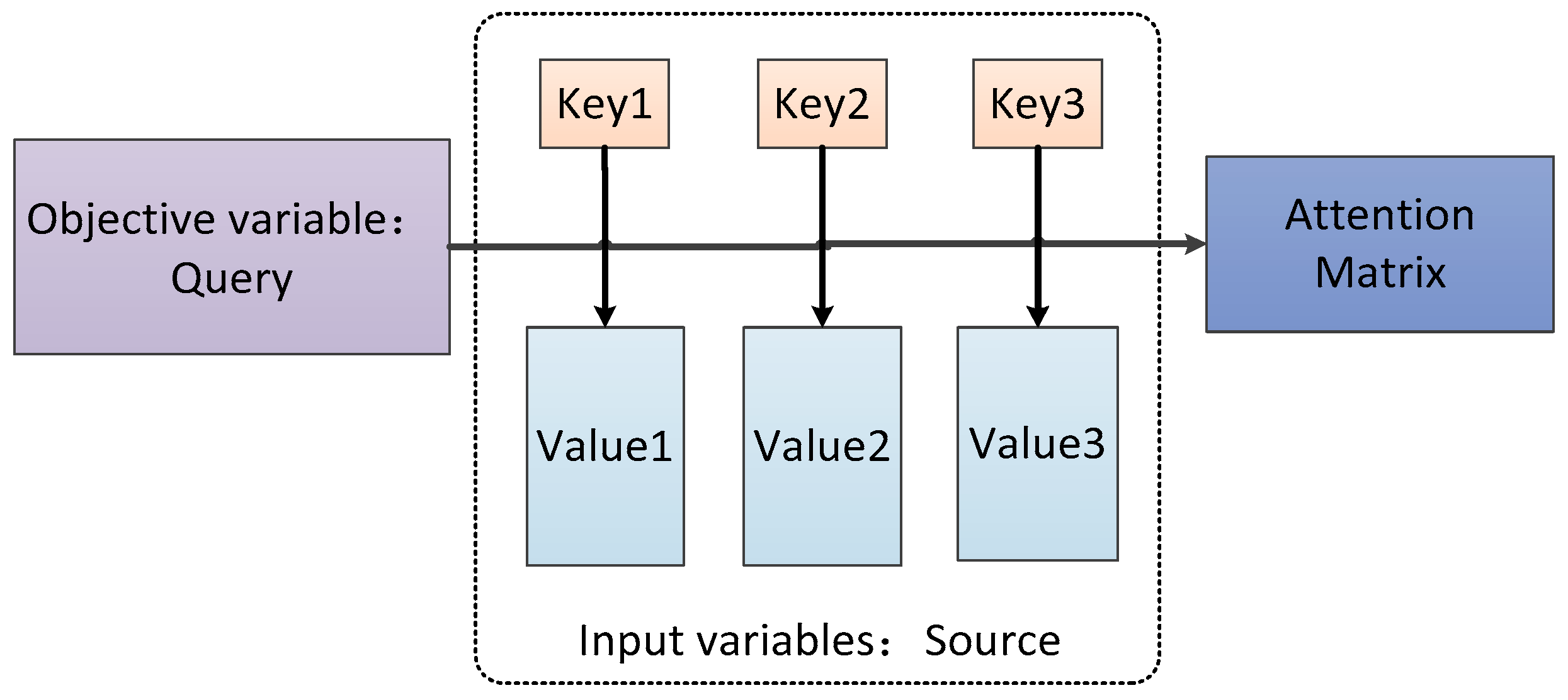
The general framework of the attention mechanism is shown in Figure 1, where the input variable is Source, the target variable is Query, and the input variable Source is abstracted into the form of key-value pairs of Key-Value. The essence of the attention mechanism is to calculate the correlation or similarity between the Key matrix in the input variable Source and the target variable Query to obtain the weight coefficient of each Key and the corresponding Value, and then perform weighted summation through the Key query Value to obtain the final attention matrix.

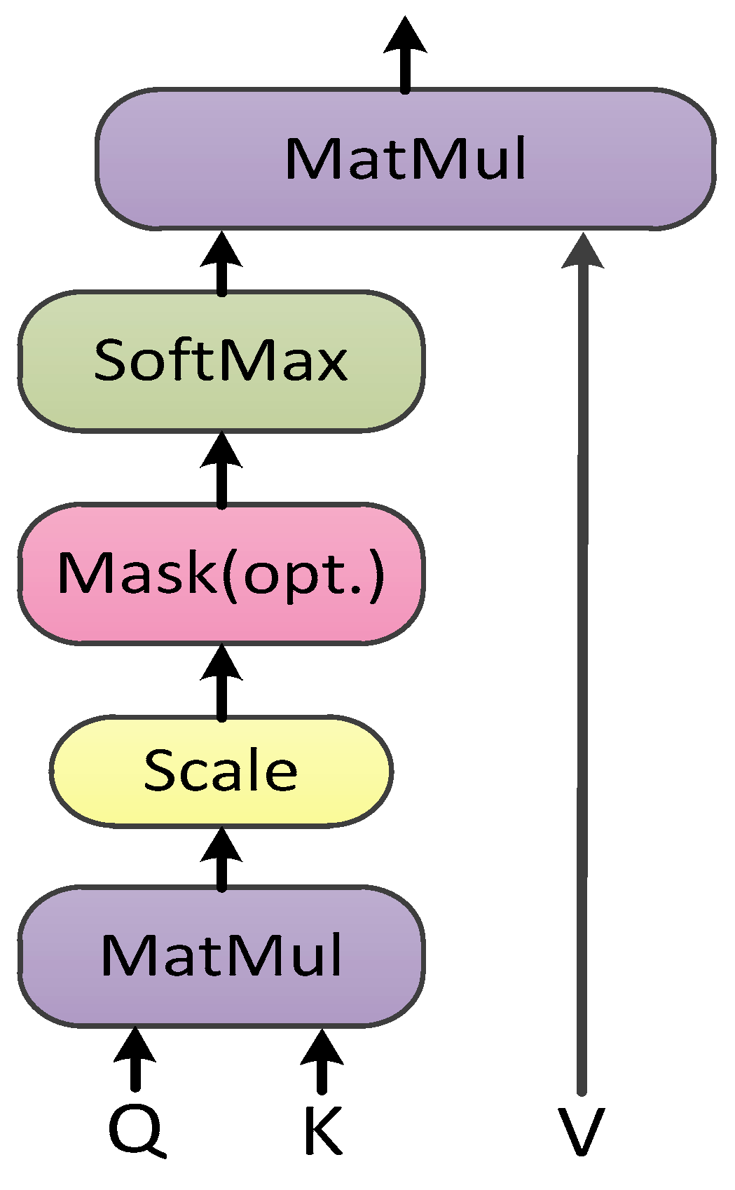
The self-attention mechanism is derived from the attention framework above and uses the inner product of the matrices to calculate the similarity. The specific calculation process is shown in Figure 2. First, the matrices Q, K, and V are obtained by a linear transformation of the input variables. Then, the inner product of the matrix Q and K is calculated and scaled, and the weights are normalized by rows. Finally, the final attention matrix is obtained by the inner product operation with the matrix V. The calculation formula is as shown in formula (1). In order to increase the diversity of self-attention, the self-attention process can be performed many times to obtain the Mul-head-attention matrix.

$$\mathrm{Attention}(\mathrm{Q},\mathrm{K},\mathrm{V})=\mathrm{softmax}(\frac{{\mathrm{QK}}^{\mathrm{t}}}{\sqrt{{\mathrm{d}}_{\mathrm{k}}}})\mathrm{V}$$

(1)

3.2. Feature Fusion

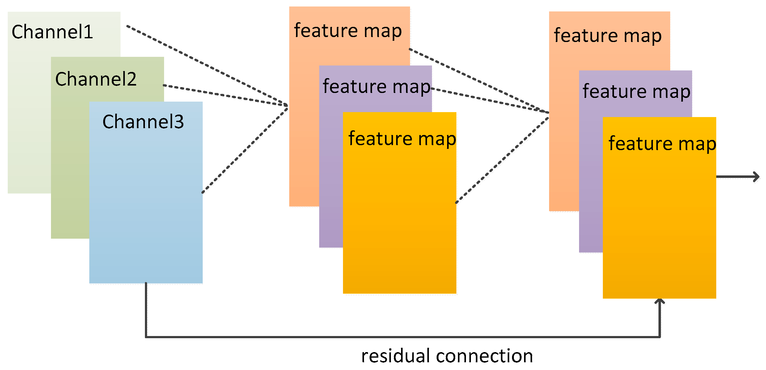
Since there are many data sources in power forecasting, including time series data of wind turbine operation, time series data of meteorological mast, and time series data of meteorological forecast, the effective fusion of features from different data sources will improve the prediction performance significantly. CNN network, as an effective method for image feature extraction, has obtained very good results since it was proposed and applied. It has become a basic unit structure in the field of image and video. In this paper, data from different sources are used as separate channels for feature fusion with CNN networks to obtain multiple feature maps on the basis of multi-source data. In addition, the risk of gradient disappearance is further reduced through residual connections, which significantly improves the feature representation after fusion of multiple sources of data. The feature fusion process based on CNN network is shown in Figure 3.

3.3. Feature Selection

Feature selection has always been a very important technical tool in the process of data mining or machine learning. On the one hand, it can reduce the influence of invalid features to speed up the model training process. On the other hand, it can reduce the impact of multi-collinearity on the accuracy of the model by eliminating invalid variables, so as to ensure that the model can still obtain better prediction results with fewer input variables. The existing methods of feature selection are based on ranking the importance of different variables over the entire time horizon to obtain the effect of feature selection. However, feature selection methods that assign weights to features at each time step are very rare. 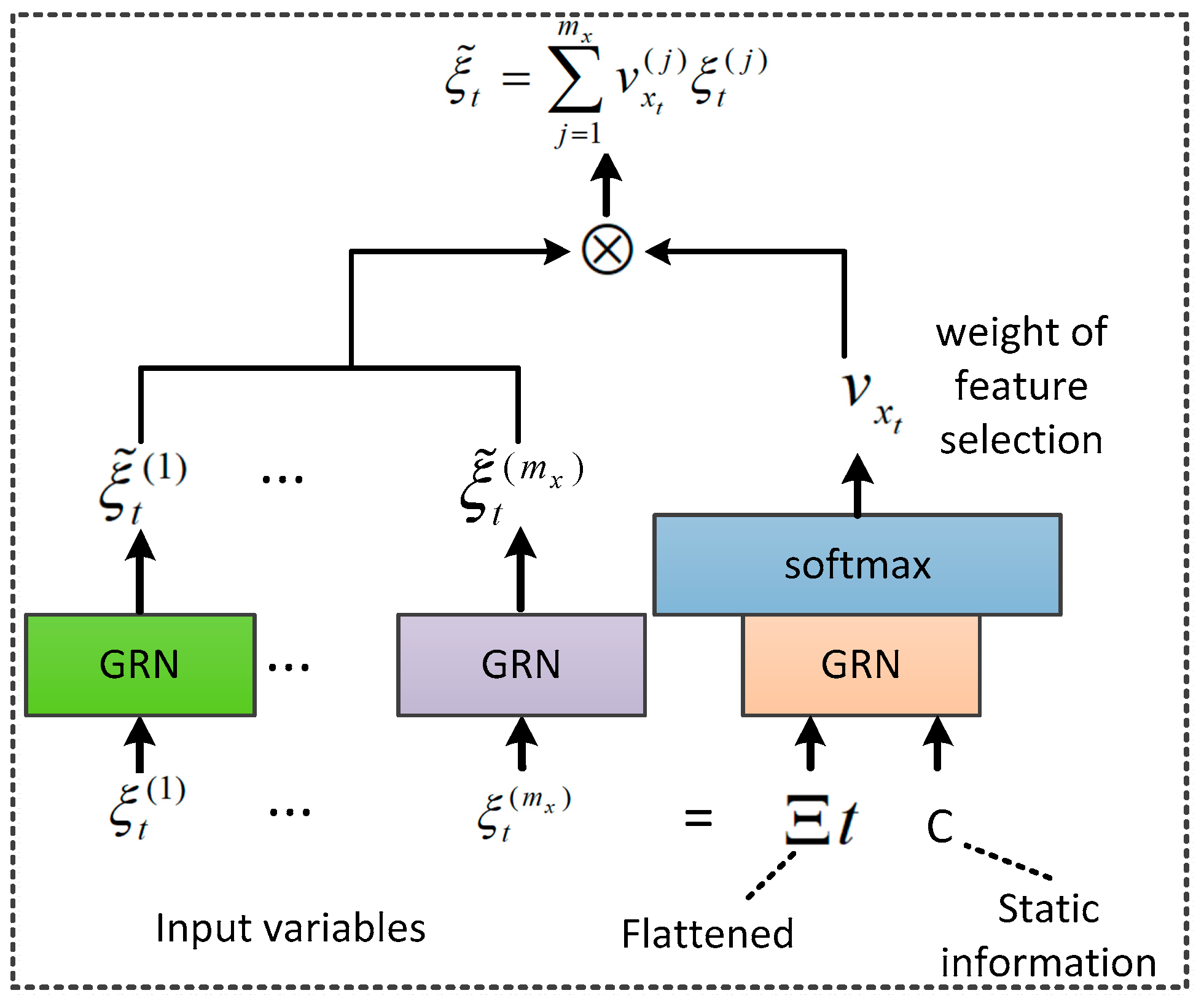An effective method for feature selection is provided in the TFT (Temporal Fusion Transformers) model [33] proposed by Bryan Lim et al. of the Google research team. The framework for feature selection in this paper is shown in Figure 4. The core idea is to use the Gated Residual Network (GRN) as a non-linear unit and apply the add-attention mechanism for feature selection. First, the d-dimensional vector of each time step is input into the GRN to add non-linear representation and the forgetting function. Then, the features of all time steps are input into the GRN to calculate the variable weights, and the weights are normalized by softmax. Finally, the elemental Hadamard product operation is performed between the weights and the feature selection results of each time step to obtain the final feature selection results.

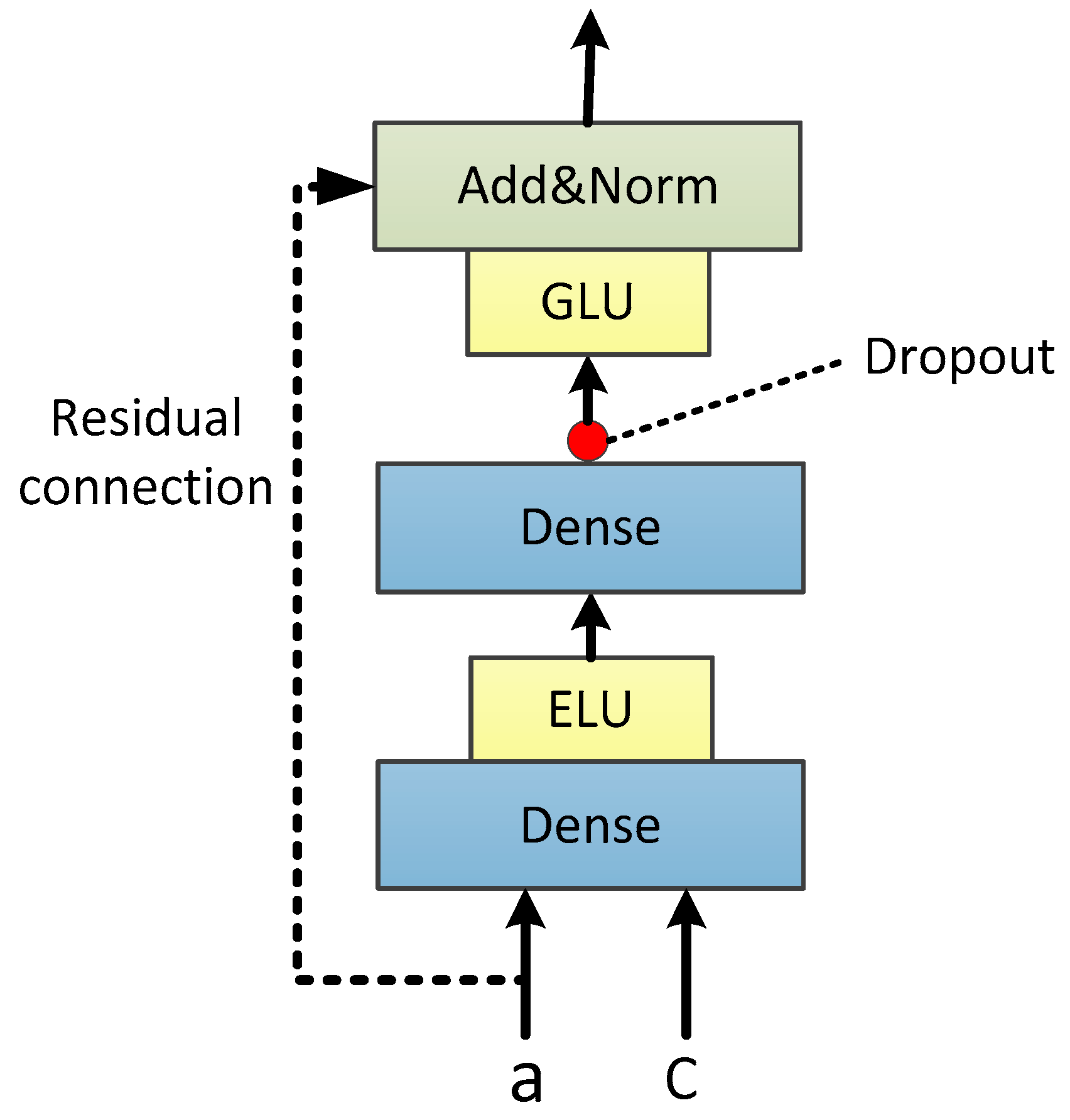
The GRN is the key point in the feature selection process described above. The network structure of the GRN is shown in Figure 5. Its calculation expression is as follows.

$${\mathrm{GRN}}_{\mathrm{w}}{(\mathrm{a},\mathrm{c})=\mathrm{LayerNorm}(\mathrm{a}+\mathrm{GLU}}_{\mathrm{w}}{(\mathsf{\eta }}_1\left)\right)$$

(2)

$${\mathsf{\eta }}_1{=\mathrm{W}}_{1,\mathrm{w}}{\mathsf{\eta }}_2{+\mathrm{b}}_{1,\mathrm{w}}$$

(3)

$${\mathsf{\eta }}_2{=\mathrm{ELU}(\mathrm{W}}_{2,\mathrm{w}}{\mathrm{a}+\mathrm{W}}_{3,\mathrm{w}}{\mathrm{c}+\mathrm{b}}_{2,\mathrm{w}})$$

(4)

where LayerNorm is the process of Residual connection and Layer Normalization. $\mathrm{a}$ represents input features, $\mathrm{c}$ is the static context information of input, GLU is the gate linear unit, ELU is the exponential linear unit, and $\mathrm{w}$ is the weight information. The calculation of GLU is as follows:

$${\mathrm{GLU}}_{\mathrm{w}}{\left(\mathsf{\gamma }\right)=\mathsf{\sigma }(\mathrm{W}}_{4,\mathrm{w}}{\mathsf{\gamma }+\mathrm{b}}_{4,\mathrm{w}}{\left)\mathrm{e}\right(\mathrm{W}}_{5,\mathrm{w}}{\mathsf{\gamma }+\mathrm{b}}_{5,\mathrm{w}})$$

(5)

Similar to the forget gate in LSTM, $\sigma (\cdot )$ is the sigmoid activation function; $\odot$ is the elemental Hadamard product. The feature oblivion effect is obtained by performing a non-linear transformation and a linear change of the input followed by an elemental Hadamard product operation.

3.4. Multi-Step Prediction

Power forecasting is divided into ultra-short-term prediction, short-term prediction, and medium- and long-term prediction. The short-term prediction requires a point-by-point forecast for the next 72 h at 15 min data resolution. Even forecasting the power for the next 24 h at 15 min data resolution requires a 96-point multi-step prediction process. The multi-step forecasting problem has always been a difficult problem in time series prediction, which restricts the further improvement of the accuracy of the model. Multi-step prediction methods can be divided into recursive prediction and direct prediction.

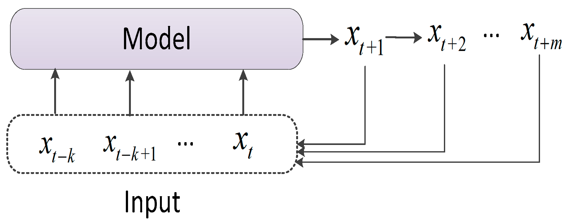
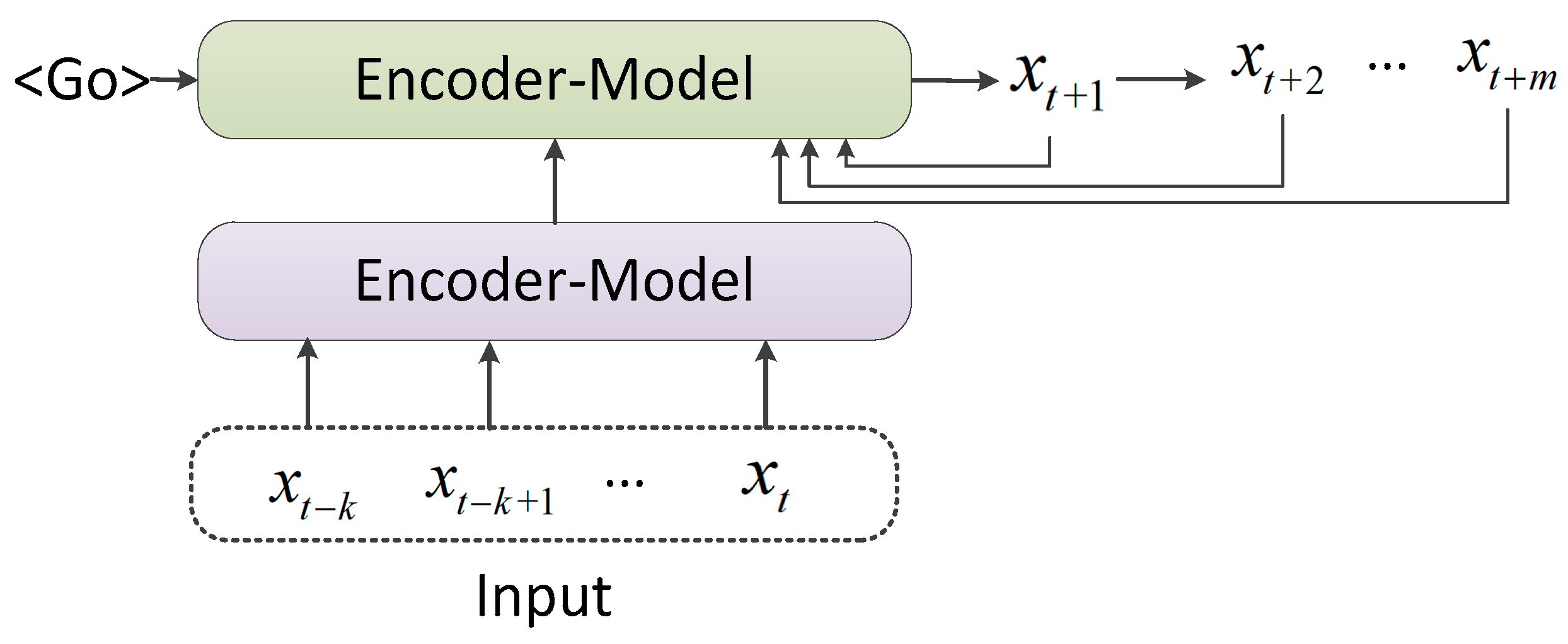
The recursive prediction method is a single-step prediction which predicts only one state at a time, and then uses the predicted state as input to predict the second future state. The recursive prediction method is simply divided into two architectures: single variable and Encoder–Decoder. The specific calculation process is shown in Figure 6 and Figure 7. The typical representative of the Encoder–Decoder architecture is the Seq2Seq+attention model. When the Seq2Seq+attention model is used for prediction, the input of the decoder is the hidden vector of the output of the encoder and the result of the previous prediction. After the attention mechanism is added, the difference in each prediction time step is increased, and the prediction accuracy has improved substantially.

The recursive prediction method is based on the correlation characteristics of the time series data context for recursive prediction. However, there are significant limitations, the prediction error of the previous step will affect the accuracy of the next step, and there is a risk of error accumulation. In addition, the prediction process is a serial process which will affect the operation efficiency.

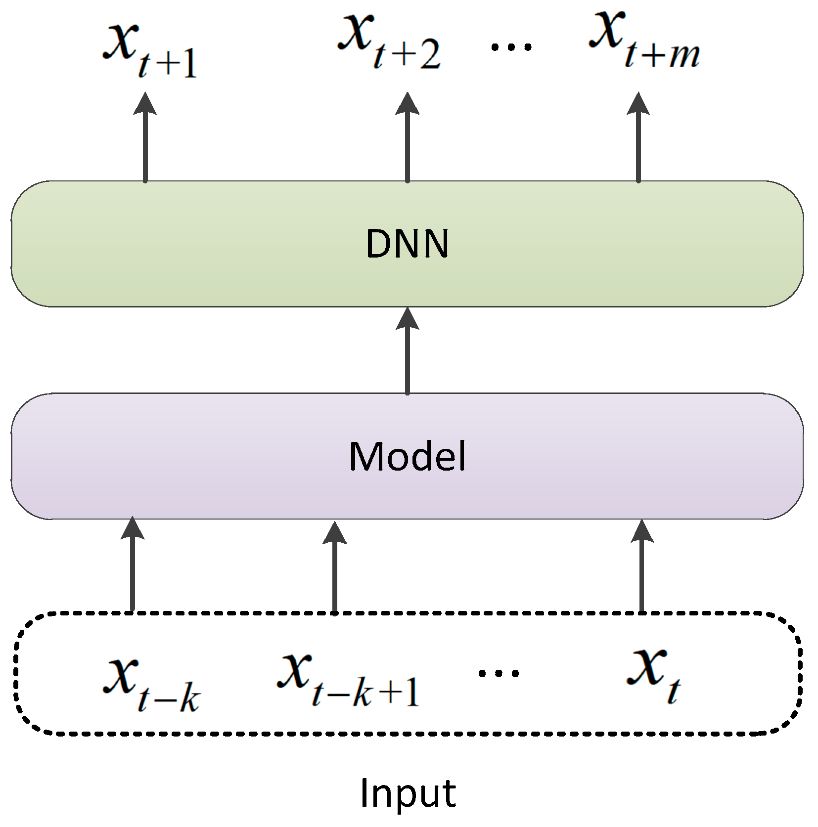
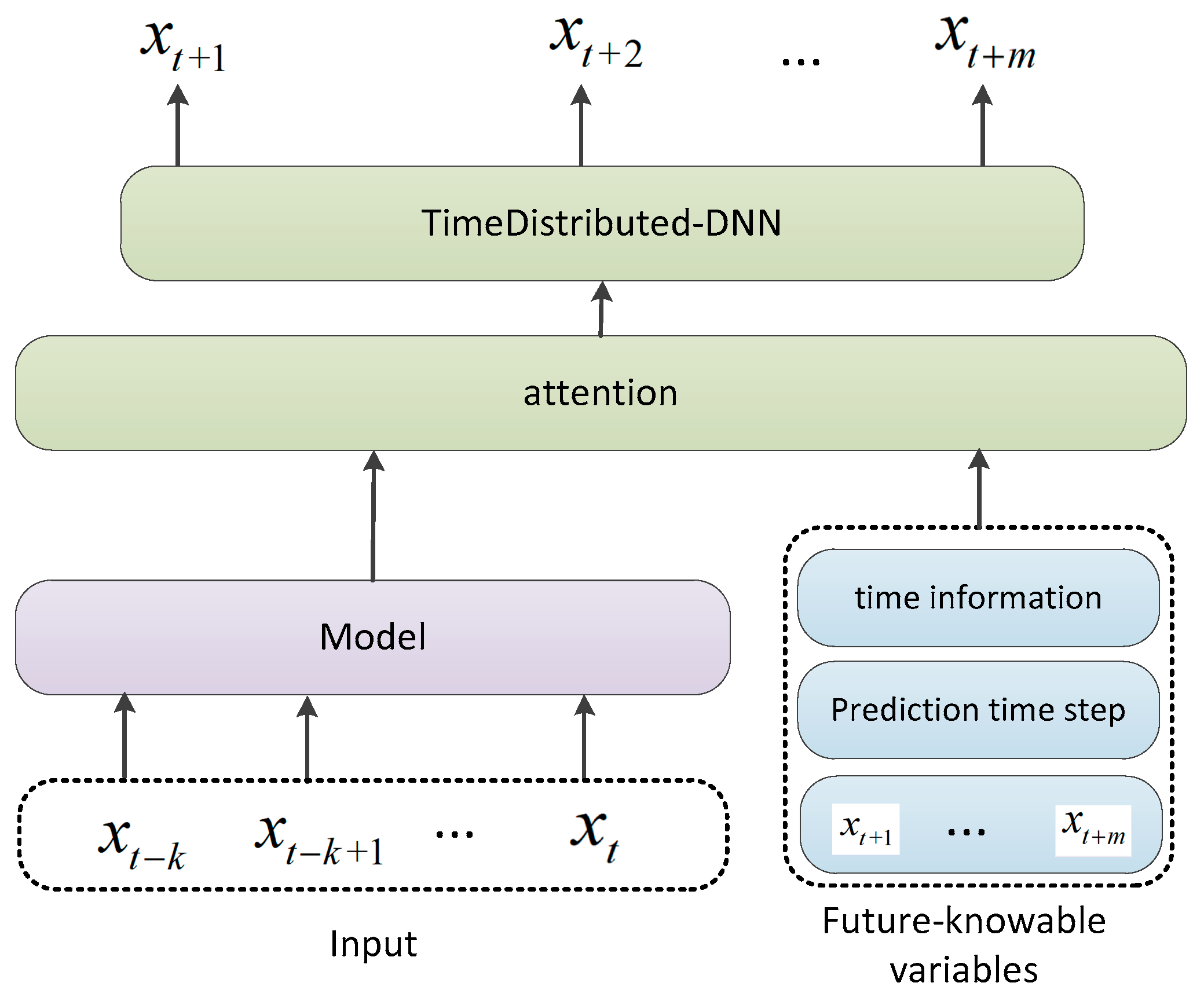
The direct prediction method is to predict the state of a future period from the historical state directly. The specific structure is shown in Figure 8. Before the attention mechanism was widely used, the direct prediction method had different implementations according to different models. If the traditional model that only receives a single sample input, such as the Xgboost model, is used, to achieve the effect of multi-step prediction, the prediction time step needs to be taken as the input before the model can learn what time step the current prediction task is. If a neural network model is used, the neurons of the last fully connected layer can be set as the number of prediction steps, and the result of multi-step prediction can be achieved directly.

The direct prediction method is simple, but it ignores the context of time series data. This problem can be effectively solved by adding an attention layer after the output layer of the model. By calculating the correlation or similarity at different times, the characteristics of different time steps can be globally characterized, so that each time step contains the state characteristics of all time steps. Therefore, the problem of context correlation in the prediction process can be alleviated to a certain extent. At the same time, the attention mechanism can capture medium- and long-distance dependencies in a short path, and it has gradually become a very important method in multi-step prediction.The specific structure is shown in Figure 9.

4. Power Forecasting Framework

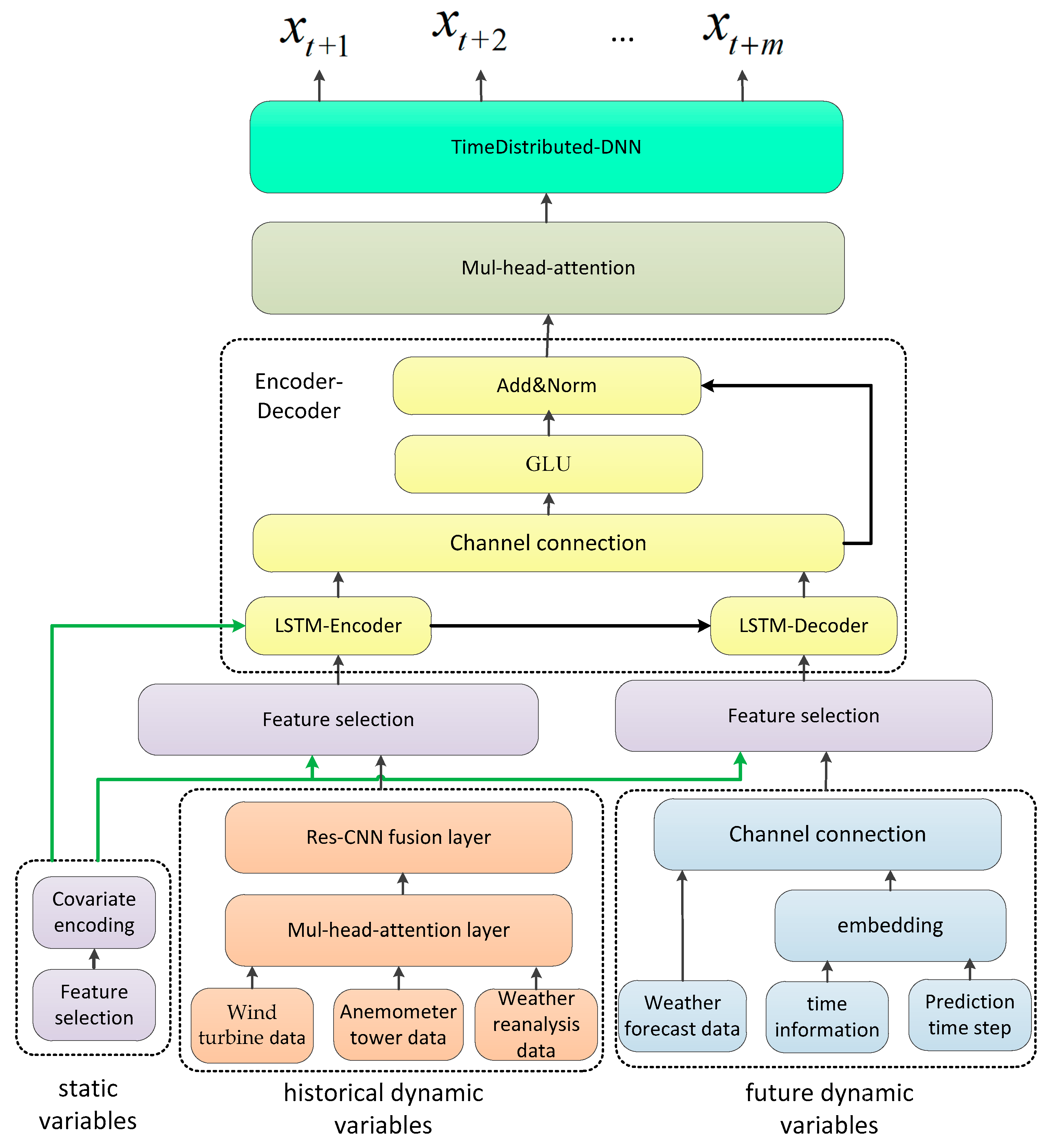
Based on the research of the above problems, the structure of the wind farm level short-term power forecasting model is designed, as shown in Figure 10. The main components of the model are the static variable module, the historical dynamic variable module, the future dynamic variable module, Encoder–Decoder architecture, the attention module, etc.

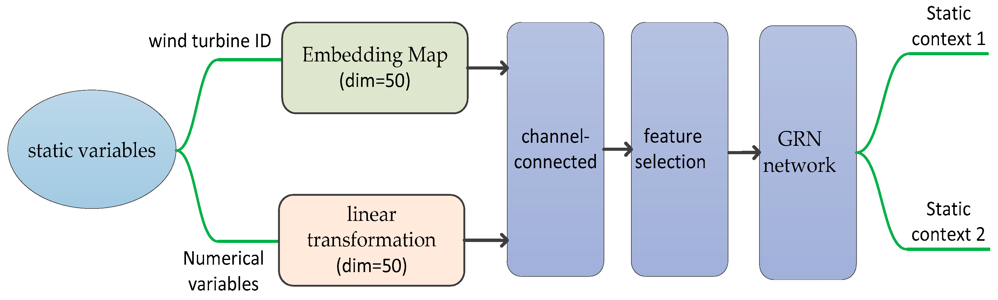
Step 1. The static variable module is mainly used for feature selection and variable coding of static variables. The detailed static variable processing is shown in Figure 11.

The static variables include wind turbine ID, longitude and latitude, and monthly and daily statistical electric quantity. First, the discrete wind turbine ID is processed by embedding, and the rest of the variables are transformed linearly. Here, the dimension of embedding and linear transformation is the same, and we give the dimension of hidden layer as 50. Every static variable is mapped to 50 dimensions. Then, the two parts of features are channel-connected and use the feature selection framework introduced in Section 3.3 to select features; finally, in order to increase the diversity of each static variable, the GRN network is used to encode the covariates for each variable, and eventually the feature representation of the static variable is obtained. The static variable can be expressed as ${\mathrm{x}}_{\mathrm{static}}\in {ℝ}^{\mathrm{K}\times \mathrm{N}}$, where K is the time step and N is the variable dimension. After the above process, the static variable is changed from ${\mathrm{x}}_{\mathrm{static}}\in {ℝ}^{\mathrm{K}\times \mathrm{N}}$ to ${\mathrm{x}}_{\mathrm{static}}\in {ℝ}^{\mathrm{K}\times \mathrm{N}\times 50}$. The two static covariate coding results are denoted as ${\mathrm{x}}_{\mathrm{sc}\_1}$ and ${\mathrm{x}}_{\mathrm{sc}\_2}$.

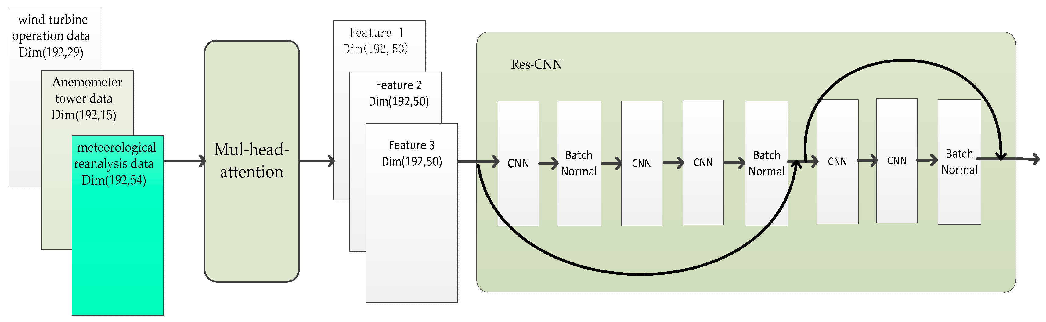
Step 2. The historical dynamic variable module includes multi-source data representation and multi-source data fusion. The detailed processing is shown in Figure 12.

The main data sources include wind turbine operation data such as power, wind speed, wind direction, rotational speed, pitch angle, ambient temperature, wind measure mast operation status, etc., as well as meteorological mast data within the wind field, such as wind speed, wind direction, and temperature at different heights. The meteorological reanalysis data adopt ERA5 data, such as decomposition wind speed, temperature, and humidity at different heights. As different data sources have different data dimensions, the Mul-head-attention layer is used to normalize the dimensions, while the global information integration is carried out to characterize the features at each time step twice. The hidden dimension of the Mul-head-attention layer is set to 50, expressed as $d_{\mathrm{model}}=50$. Then, the features from different data sources represented by the Mul-head-attention layer are used as separate channels.

$${\mathrm{Multihead}(\mathrm{Q},\mathrm{K},\mathrm{V})=\mathrm{concat}(\mathrm{head}}_{\mathrm{WT}}{,\mathrm{head}}_{\mathrm{AT}}{,\mathrm{head}}_{\mathrm{NWP}})$$

(6)

where ${\mathrm{head}}_{\mathrm{WT}}$ is the characterization result of wind turbine operation data; ${\mathrm{head}}_{\mathrm{AT}}$ is the characterization result of meteorological mast data; ${\mathrm{head}}_{\mathrm{NWP}}$ is the characterization result of meteorological reanalysis data.

$${\mathrm{head}}_{\mathrm{WT}}{=\mathrm{selfattention}(\mathrm{x}}_{\mathrm{WT}}{\mathrm{W}}_{\mathrm{i}}^{\mathrm{Q}}{,\mathrm{x}}_{\mathrm{WT}}{\mathrm{W}}_{\mathrm{i}}^{\mathrm{K}}{,\mathrm{x}}_{\mathrm{WT}}{\mathrm{W}}_{\mathrm{i}}^{\mathrm{V}})$$

(7)

where the projections are parameter matrices ${\mathrm{W}}_{\mathrm{i}}^{\mathrm{Q}}\in {ℝ}^{\mathrm{dmodel}\times \mathrm{dwt}}$, ${\mathrm{W}}_{\mathrm{i}}^{\mathrm{K}}\in {ℝ}^{\mathrm{dmodel}\times \mathrm{dwt}}$, ${\mathrm{W}}_{\mathrm{i}}^{\mathrm{V}}\in {ℝ}^{\mathrm{dmodel}\times \mathrm{dwt}}$. Additionally, the Res-CNN layer is used to fuse multi-source features, which in turn leads to feature enrichment. The multi-source features are denoted as $\mathrm{historical}\_\mathrm{feature}$.

Step 3. Input data of the future dynamic variable module include future weather forecast data (here, ERA5 data are used as prediction data), time information such as month, day, and hour, and prediction time steps such as values from 1 to 96 similar to position information. The time information and prediction time step are embedding-coded, and then channeled to the future weather forecast data.

$${\mathrm{future}\_\mathrm{feature}=\mathrm{concat}(\mathrm{x}}_{\mathrm{NWP}}{,\mathrm{ed}}_{\mathrm{time}})$$

(8)

Step 4. The Encoder–Decoder architecture includes the Encoder–Decoder process, the GLU, and the residual connection section. First, the feature selection is needed before encoding and decoding. Historical dynamic variables and future dynamic variables enter the feature selection framework together with static variables to achieve the feature selection function.

$${\mathrm{GRN}}_{\mathrm{w}}{(\mathrm{f}}_{\mathrm{j}}{,\mathrm{c})=\mathrm{LayerNorm}(\mathrm{f}}_{\mathrm{j}}{+\mathrm{GLU}}_{\mathrm{w}}{(\mathsf{\eta }}_1\left)\right)$$

(9)

where ${\mathrm{f}}_{\mathrm{j}}$ is the feature extracted by the upper network, such as $\mathrm{historical}\_\mathrm{feature}$ and $\mathrm{future}\_\mathrm{feature}$. $c$ is static covariate coding result such as ${\mathrm{x}}_{\mathrm{sc}\_1}$. The feature selection results of historical dynamic variables and future dynamic variables are denoted as $\mathrm{historical}\_\mathrm{fs}$ and $\mathrm{future}\_\mathrm{fs}$. Then, the static variables are used as the initial state of the encoding LSTM layer, and the historical dynamic variables are used as the input to encode; the encoded last hidden variable is used as the initial state of the decoding LSTM, and the future dynamic variable is used as the input for decoding. The dimension of the LSTM model output space is 50. The output results of the encoder and the decoder are connected by channels to obtain $\mathrm{lstm}\_\mathrm{feature}$.

$$\begin{array}{l}{\mathrm{lstm}\_\mathrm{feature}=\mathrm{concat}\left(\mathrm{Lstm}\right(\mathrm{historical}\_\mathrm{fs},\mathrm{x}}_{\mathrm{sc}\_2}),\\ \mathrm{Lstm}(\mathrm{future}\_\mathrm{fs},\mathrm{state}\_\mathrm{h}, \mathrm{state}\_\mathrm{c}))\end{array}$$

(10)

Subsequently, the $\mathrm{lstm}\_\mathrm{feature}$ is input to GLU to realize the characteristic memory and forgetting process. Finally, the residuals are connected and normalized by Layer Normalization.

Step 5. The attention module uses the Mul-head-attention layer to characterize the characteristics of different time steps and obtains the relationship between each time step and the global time, which improves the prediction accuracy.

Step 6. The fully connected layer with Time Distributed is used to predict each prediction time step, and the multi-step power forecasting result is obtained.

5. Case Analysis

5.1. Dataset Introduction

A wind farm in northwestern China is used to verify the model; the scale of the wind farm is 23 Wind turbines, data range from May 2022 to October 2022, and the data duration is about 180 days. Data sources include operation data of wind turbines, data of meteorological mast, and meteorological reanalysis data.The data are shown in

Table 3. Dataset description.

Datasets	Source of Data	Data Resolution (min)
Operating data of wind turbines	Scada	15
Meteorological mast	Observation sensors	15
Meteorological reanalysis data	ERA5	60

.

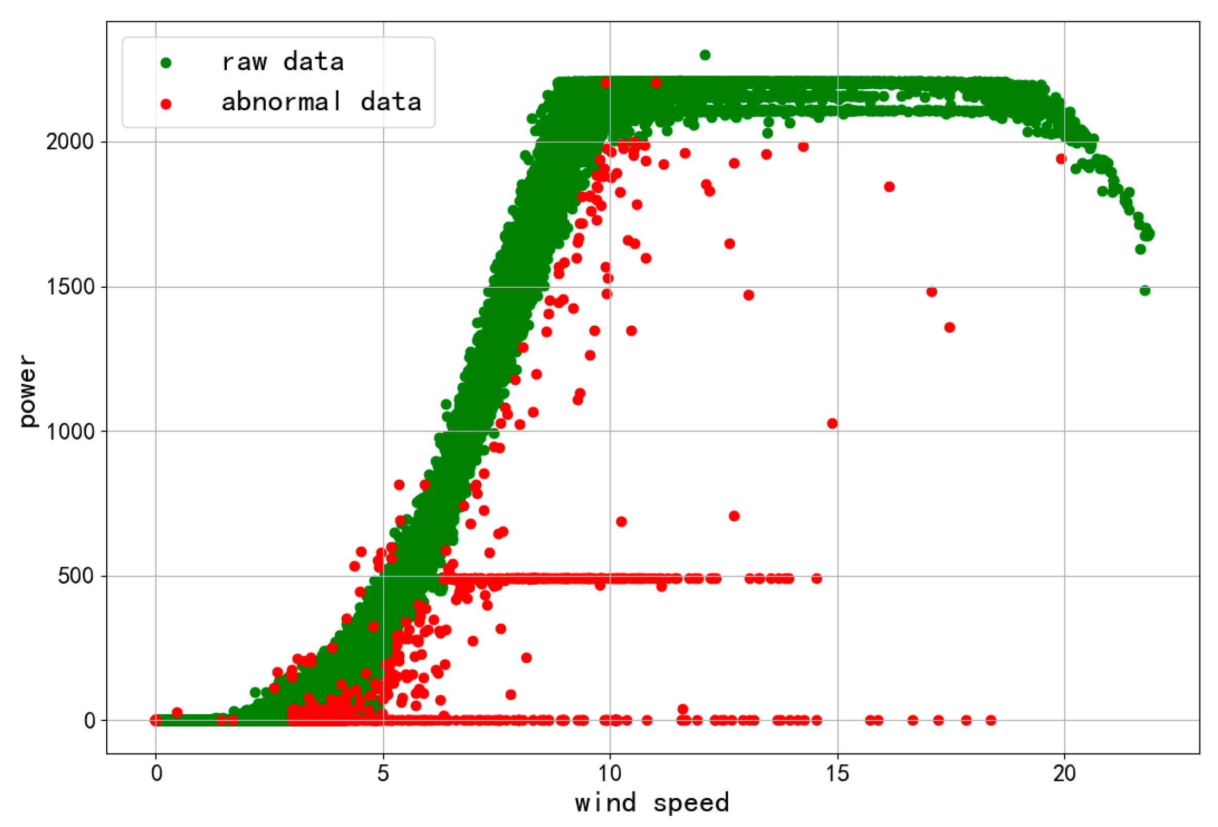
The scatter plot of one wind turbine is shown in Figure 13. The model architecture in Section 3 is used to complete the field-level short-term power forecasting function; that is, it is used to predict the future 24 h with a point-by-point prediction at a temporal resolution of 15 min. A deep learning model is established for the whole wind farm, and the short-term power prediction results of each wind turbine are obtained by distinguishing the characteristics of different wind turbines through the information of the wind turbine ID, longitude, and latitude.

5.2. Hardware Environment

The model verification is based on the Tensorflow framework and implemented by Keras. Tensorflow version 2.10.0 and Keras version 2.10.0are implemented; GPU resources are NVIDIA Tesla GPU, there are 4 blocks in total, and each block has 32GB of memory.

5.3. Benchmark Model and Evaluation Criteria

The TFT model and the Seq2Seq+attention model are used as benchmark models to compare with the model proposed in this paper. In the modeling process of the TFT model, the historical variables do not use the Res-CNN network for feature fusion, but only connect multi-source data channels to verify the promotion effect of feature fusion on the model. The Seq2Seq+attention model retains the feature fusion part of the Res-CNN network and replaces the attention part of this paper with the additive attention mechanism in the Seq2Seq+attention model to compare the similarities and differences between recursive and direct prediction. The biggest difference among the three models is multi-source data fusion and the multi-step prediction strategy. The difference is shown in

Table 4. Description of the benchmark model.

Model	Feature Fusion or Not	Multi-Step Prediction Mechanism
Proposed Model	Y	direct prediction
TFT	N	direct prediction
Seq2Seq	Y	recursive prediction

.

The model evaluation criteria include Root Mean Square Error (RMSE) and Mean Absolute Error (MAE). The calculation of RMSE and MAE is shown below:

$$\mathrm{RMSE}=\sqrt{\frac{1}{\mathrm{n}}{\displaystyle \sum _{\mathrm{i}=1}^{\mathrm{n}}{{(\mathrm{y}}_{\mathrm{i}}{- \hat{\mathrm{y}}}_{\mathrm{i}})}^2}}$$

(11)

$$\mathrm{MAE}=\frac{1}{\mathrm{n}}{\displaystyle \sum _{\mathrm{i}=1}^{\mathrm{n}}\left|{\mathrm{y}}_{\mathrm{i}}{- \hat{\mathrm{y}}}_{\mathrm{i}}\right|}$$

(12)

5.4. Analysis of Prediction Results

This validation is based on the real wind turbine dataset from May 2022 to October 2022, and the data duration is about 180 days. The historical data of two days is used to predict the power of the next day. In order to increase the sample size, the time window method was used to construct the sample, and the sliding time step was 15 min. Since the number of wind turbines is 23, the total sample size is approximately 23 × (180 × 24 × 60/15) = 397,440. A total of 80% of the data is used for model training, with a sample size of about 317,952. A total of 20% of the data is used for model testing, with a sample size of about 79,488. The prediction performance of the three models will be tested on the test set.

5.4.1. Comparison of Convergence Rates in Training Sets

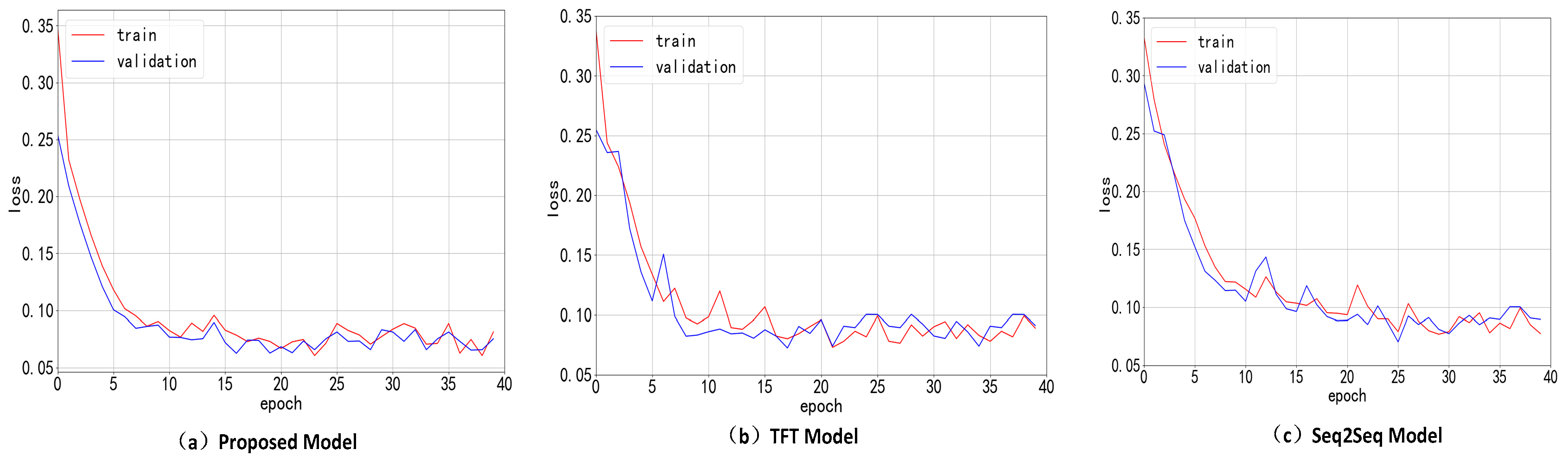
For the convenience of comparison, this section takes a single wind turbine as the original dataset for model training. The convergence speed of the three models under the same dataset of a single wind turbine is compared. The model parameters are shown in

Table 5. Performance comparison of single wind turbine model.

Models	Parameters	Value
Proposed Model	Feature selection: dimension	50
	Multi-head-attention: head dimension	50
	Res-CNN: filters number	20
	LSTM: hidden layer size	50
	Dropout	0.1
	Learning rate	0.01
	Optimizer	Adam
	Batch size	32
	Epochs	100
TFT	Feature selection: dimension	50
	LSTM: hidden layer size	50
	Dropout	0.1
	Learning rate	0.01
	Optimizer	Adam
	Batch size	32
	Epochs	100
Seq2Seq	Feature selection: dimension	50
	Multi-head-attention: head dimension	50
	Res-CNN: filters number	20
	LSTM: hidden layer size	50
	Dropout	0.1
	Learning rate	0.01
	Optimizer	Adam
	Batch size	32
	Epochs	100

, and the loss function changes during model training are shown in Figure 14.

The model training results are shown in

Table 6. Performance comparison of single wind turbine model.

Types		Proposed Model	TFT	Seq2Seq
parameters		1.292 million	2.426 million	2.041 million
RMSE < 0.1	MAE	0.0841	0.0989	0.0998
	Time required	9.97 min	19.32 min	37.8 min
Optimal model	MAE	0.0641	0.0833	0.0875
	RMSE	0.0677	0.0853	0.0878
	Time required	21.67 min	27.48 min	81.2 min

.

It can be seen from the comparison in Table 2:

(1) In terms of model complexity, the parameters of the proposed model are significantly less than the comparison model, and the proposed model is simpler, which reduces the risk of model overfitting.

(2) In terms of the convergence speed of the model, by setting the RMSE of the training set less than 0.1 for the first time as the criterion, the model in this paper has the fastest convergence speed. Both the proposed model and the TFT model use a direct prediction mechanism for multi-step prediction, while the Seq2Seq+attention model uses a recursive prediction mechanism to accomplish multi-step prediction. It can be seen that the training speed of the direct prediction mechanism is significantly faster than that of the recursive prediction mechanism.

(3) In terms of the performance of the optimal model, the prediction effect of the validation set is taken as the standard, and the proposed model in this paper obtains the best prediction effect with the fastest speed. Under the same multi-step prediction mechanism, the prediction effect of the proposed model using the Res-CNN network for feature fusion is better than that of the TFT model, which verifies the improvement of the prediction performance of the Res-CNN network feature fusion. Under the same Res-CNN network feature fusion mechanism, the direct prediction mechanism of the proposed model is better than the Seq2Seq+attention model, which verifies the effectiveness of the direct prediction mechanism.

5.4.2. Comparison of Model Generalization Ability

To demonstrate the generalization ability of the model, the trained model is applied to our testing dataset, and results are compared with the benchmark models. The performance evaluation metric is calculated for each wind turbine, and the results are given in

Table 7. Model generalization ability analysis.

Types		Proposed Model	TFT	Seq2Seq
Time of training		3.2931 h	5.9437 h	14.625 h
RMSE	MAX	0.2011	0.2856	0.2908
	MIN	0.0585	0.1029	0.0997
	Mean	0.1243	0.1501	0.1487
MAE	MAX	0.0707	0.0891	0.0844
	MIN	0.0061	0.0106	0.0099
	Mean	0.0176	0.0248	0.0234

.

According to Table 7, the proposed model performs the best in the power prediction of multiple wind turbines in the wind farm, with an average RMSE of 0.0585. It is superior to other comparison models and provides an effective method for power forecasting.

6. Conclusions

In this work, we tackle the multi-step prediction problem for wind power, and a method based on multi-source data fusion and deep learning algorithmic architecture is proposed. The following conclusions can be made through the comparative analysis using operational wind farm data:

(1) The accuracy of the forecasting model can be further improved by making full use of static variable information and combining it with time varying information for feature selection. At the same time, more statistical static variables can integrate historical statistical information into the model to improve the predictive ability of the model.

(2) Multi-source data fusion with Res-CNN can effectively improve the generalization ability of the model, and using multi-source data fusion for feature engineering based on the same dataset can increase the forecasting skill of the model.

(3) The direct prediction method combined with the self-attention mechanism can achieve satisfactory skill in multi-step prediction problems. Compared with the recursive prediction method, it has shown advantages in training speed and prediction accuracy.

The deep learning prediction model proposed in this paper achieves better results than the Seq2Seq+attention model in our numerical experiment of wind farm power forecasting. However, in the multi-step prediction problem of power forecasting, there is still a significant time lag in the prediction results when there are extreme gusts. In addition, there are still some important variables, such as division of working conditions, which have not been considered in this study, but they are believed to significantly affect performance of such data-driven forecasting methods. These remain our further research questions.