Numerical Validation of a New Analytical Solution for Helical (Earth-Basket) Type Ground Heat Exchangers

Abstract

In this paper, we show that an analytical solution based on the Finite Line Source and G-function approach is both sufficiently fast and accurate for design calculations of ground heat exchangers with a complex (spiral) geometry. Detailed validations were performed for the steady-state and transient responses of analytical models with different time scales (10 h and 250 h). A comparison with a detailed computational fluid dynamics model (Ansys Fluent) and the analytical method for different boundary conditions showed a very good agreement (maximum root mean square error) smaller than 0.25 K.

1. Introduction

Ground source heat pumps use the ground as a source or sink of heat. Owing to the relatively amiable temperatures in the ground and the lack of requirement for defrosting cycles, they achieve better overall performance compared with air source heat pumps. Moreover, ground source heat pump systems offer the possibility of direct or passive cooling (without the use of the heat pump). The ground stores the low and high temperatures diurnally and seasonally, and a well-designed system achieves high performance with low or no maintenance and a long operational life of 50 years or more.

Owing to the storage of high and low temperatures in the ground, the ground temperature reflects the history of energy exchange. While the source temperature of an air-source heat pump only depends on the ambient temperature, the source temperature of a ground source heat pump depends on energy exchange with the ground in both the short term (heat pump operating cycles) and the long term (seasonal energy exchange over the operational life). This behaviour needs to be accounted for in the design of the system, which is, therefore, more challenging than designing an air source heat pump or gas boiler system.

The design of a ground heat exchanger is a critical factor in the implementation of a ground source heat pump system, as it is a significant cost factor. In many cases, a vertical borehole heat exchanger is selected, as it offers good performance for a small footprint, but it is relatively costly due to the drilling cost. When sufficient space is available and the energy demand profile of the project permits, other ground heat exchangers, such as horizontal, ring collectors (also called slinky) or spiral type collectors (also called earth basket collectors) can be considered.

Adequate design methods have been developed for vertical borehole heat exchangers [1,2], horizontal heat exchangers [3] and ring collector (also called slinky) ground heat exchangers [3,4]. For spiral or earth basket heat exchangers, although some analytical solutions have been discussed in the literature (e.g., [5,6,7]), so far, no suitable analytical solutions that can be integrated into an engineering design tool are available.

Within the framework of the EU program “Horizon 2020”, in the “GEOFIT” project [8], this has been addressed and an integrated ground source designer’s toolkit including all types of ground heat exchangers has been developed. For all types of ground heat exchangers, the engineering tool uses the well-known finite line source approach [9] for the calculation of temperature evolution on the ground heat exchanger wall. Multiple ground heat exchangers can be evaluated using a spatial superposition technique and computational efficiency is achieved by using the G-function approach [1,10] (the procedure of using the FLS with the G-function approach is discussed in more detail in Appendix B).

For most ground heat exchangers, such as vertical, horizontal and ring-collector ground heat exchangers, the validation of the implemented analytical solutions is fairly straightforward in comparison with existing engineering tools, such as Earth Energy Designer [11] and Glhepro [3]. These validations were performed as part of the development of the toolkit [9]. However, for spiral-type heat exchangers, a novel three-dimensional implementation of the FLS was developed, where the spiral shape of the ground heat exchanger was approximated by a stack of rings [9]. For the detailed validation of this analytical solution, a helical ground heat exchanger was modelled in detail using a computational fluid dynamics (CFD) simulation tool (ANYS-FLUENT). This CFD model itself was calibrated and validated using sandbox experiments [12,13].

Using the CFD model and analytical solution, validation was carried out for the steady-state situation (to validate the long-term behaviour of the analytical solution) [14]. In that paper, a comparison between the CFD and analytical FLS solutions was carried out by comparing the solution of the temperature obtained for a point cloud around the spiral heat exchanger. This approach was selected because the geometry of the analytical solution did not exactly mirror the CFD model (stack of rings vs. actual spiral geometry) and the goal was to compare individual spiral turns (or rings) in three dimensions to analyse the effects of construction parameters, such as pitch and ring diameter. In the present study, for the short-term behaviour with a time scale ranging from minutes to hours, the transient behaviour of the analytical solution is the focus. This compares the actual average spiral heat exchanger wall temperature. The parameters that were varied were the heat injection rate and soil thermal conductivity. A steady-state solution for the actual heat exchanger wall temperature was also evaluated.

Shallow Heat Exchanger Types

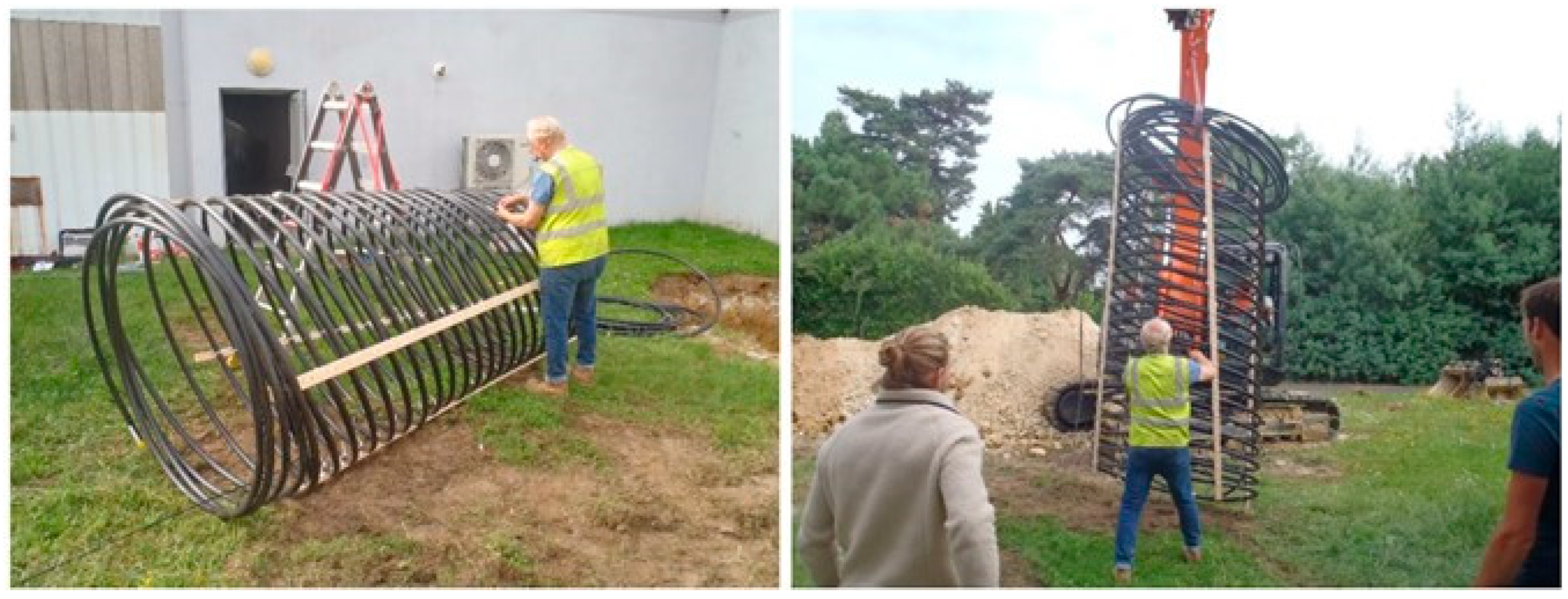
Within the framework of the Geofit project, several types of shallow heat exchangers have been installed and will be field tested, in addition to vertical borehole heat exchangers. In the Perugia (Italy) demo site. a so-called slinky or ring-collector ground heat exchanger has been installed, and in the Bordeaux (France) demo site, a spiral or earth basket heat exchanger has been installed. Figure 1 shows this installation of a spiral (earth basket) ground heat exchanger. At these field demo sites, performance data are being collected using fibre-optic distributed temperature sensing.

For the spiral coil ground heat exchanger, there is limited modelling experience, especially with analytical models suitable for use in an engineering environment. Spiral or coil heat exchangers have received attention in the literature for application in pile (foundation) heat exchangers [5,15,16], as well as in horizontally oriented spiral heat exchangers [7]. The inner pile region may be ignored by these models, treating the pile as hollow. As the thermal properties of the pile are very different from the thermal properties of the ground, these models are less suited for vertically oriented spiral heat exchangers installed not in foundation piles, but directly in the ground. This is especially true when the spiral (ring) diameter is relatively large, as in earth basket heat exchangers. A solution for a ring collector (slinky) heat exchanger is described in [6], consisting of a series of rings in a horizontal plane and based on a ring source in an infinite medium. Here, the temperature change of a ring source is obtained by integrating all contributions of point sources on the ring circumference. By applying Green’s function, the necessary point source solutions are calculated. An isothermal surface boundary condition is obtained by using mirror sources. Finally, the superposition of the solution of the individual rings obtains solutions for multiple ring cases. The analytical models used for the simulation of ring collector (slinky) heat exchangers were significantly improved by [4] considering the heat exchanger tube diameter and introducing a G-function approach to improve computational efficiency.

Using a numerical model, [17] evaluated geometric factors (mainly pitch and diameter) in terms of the thermal performance of a horizontal-spiral ground heat exchanger. The main conclusions supported the conclusions of the steady-state study of the FLS presented here [14]. However, in design studies, the solution based on COMSOL multiphysics presented in that paper is not suitable. In [18], the authors noted that there were no plain and established methods to evaluate the energy performance of truncated cone and spiral coil ground heat exchangers. Apart from numerical studies, reference is made to studies using Green’s functions, but those were aimed at pile- and borehole heat exchangers. In [18], the authors remarked that many analytical solutions consider the heat source constant over the length of the heat exchanger, which may be less suited for dynamic analysis. In [19], a 3-D simulation of the heat transfer rate in geothermal pile-foundation heat exchangers with a spiral pipe configuration is presented. Again, a numerical approach was used, which was not suited for engineering practice.

The advantages of using the finite line source approach presented in this paper are that it is already used in engineering design software for other types of ground heat exchangers, that it is sufficiently fast for engineering practice and that it can be readily combined with, e.g., analytical solutions for seasonally varying near-surface temperatures by superposition.

2. Materials and Methods

The analytical finite line source (FLS) model is based on an extension of the essentially two-dimensional ring-collector model developed [4] for horizontally and vertically oriented ring collector (also known as slinky) ground heat exchangers to a three-dimensional (3D) solution for groups of vertically oriented spiral heat exchangers. A single-spiral heat exchanger is represented by a series (stack) of ring sources that are all separated by a certain distance (pitch). Several parallel spiral heat exchangers can be installed in a single system.

The FLS solution uses spatial superposition, where the temperature effects calculated for a single source are summed (superposed) with the effects of other sources to calculate the total temperature evolution of a ground heat exchanger. The superposition principle is valid if only heat conduction is considered and if the boundary conditions are linear. In addition to spatial superposition, there is also temporal superposition applied. As the FLS calculates the effect of a constant heat rate only, time-varying heat rates are solved by the decomposition of the heat rate profile over time, calculating the temperature change due to those heat rate changes and adding these over time (see [1] for details on this methodology). In practice, calculating the temperature effect of multiple sources with a time step of one month for a total period of 30 years or more is computationally intensive. To increase computational efficiency, a G-function approach [1] is used. The G-function calculates a characteristic response of a complete heat exchanger system for one constant heat rate change (using the FLS method) and subsequently uses this characteristic G-function to solve for the complete time domain considered [1,4,10].

The FLS/G-function solution has been implemented, together with solutions for vertical boreholes, horizontal heat exchangers and slinky heat exchangers, in a consolidated engineering tool implemented in the Python programming language. Additional features implemented in the engineering toolkit are:

• Inclusion of near-surface seasonal temperature effects;
• Consideration of temperature-dependent fluid properties—this is especially relevant for fluid-to-ground-thermal-resistance calculations;
• Implementation of a detailed thermal resistance model and evaluation of critical Reynolds numbers for different geometries and definition of transition zones from laminar to turbulent flow;
• Consideration of the thermal interactions between neighbouring systems.

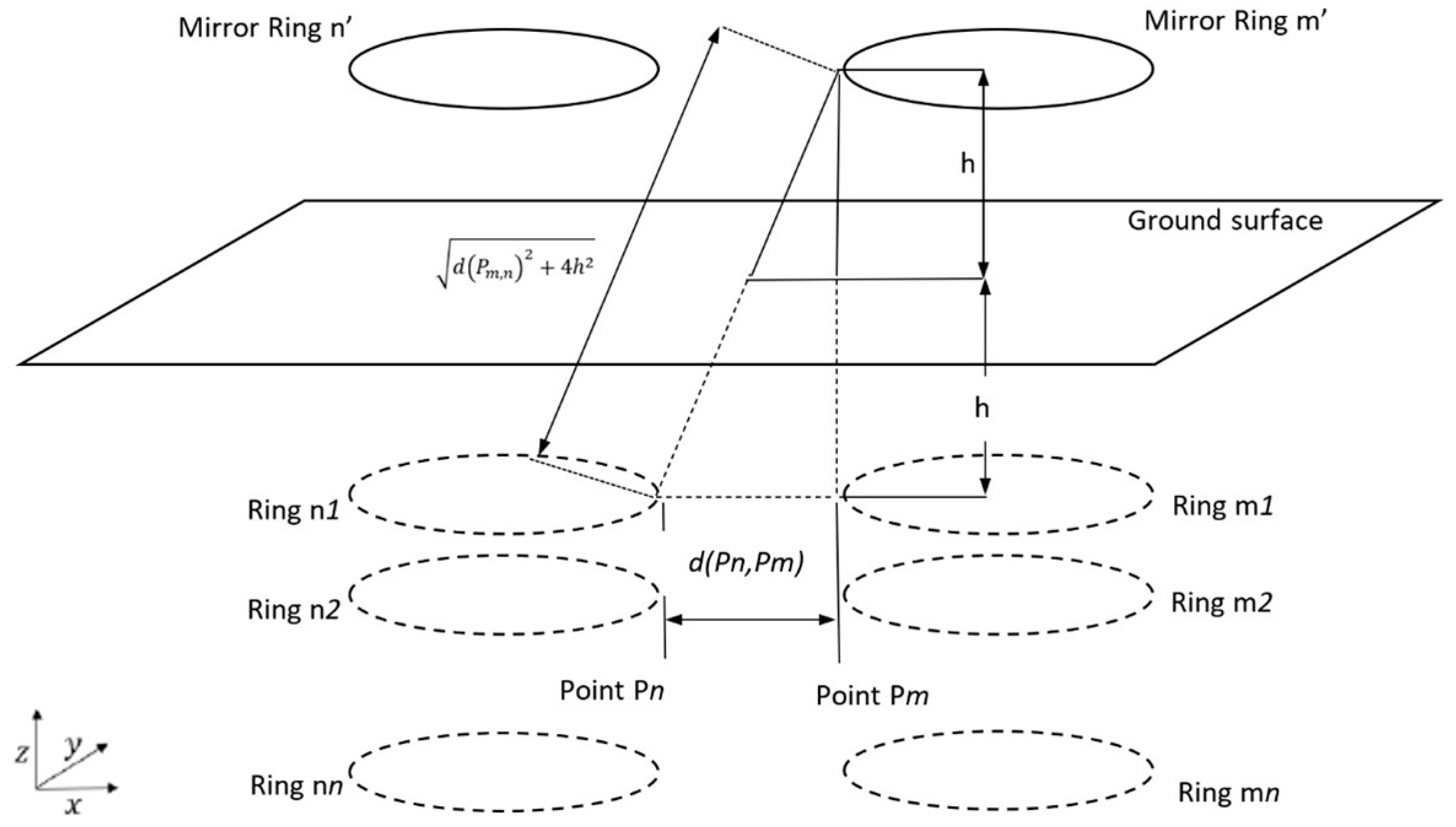
The principle of the FLS methodology (details of the FLS analytical solution for spiral heat exchangers are provided in Appendix B) is to define the geometry of the ground heat exchanger to be evaluated as a series of point sources with a constant energy flux and integrate them over the geometrical shape. On the ground surface, an isothermal temperature boundary condition is specified by defining mirror sources with an equal heat flux with an opposite sign. In our implementation (Appendix B), the earth basket spiral ground heat exchanger is simplified to a stack of rings with a constant distance (pitch) between the rings. Although this is a simplification of the actual helical geometry, the error introduced to the heat exchanger tube wall itself or at any significant distance from the heat exchanger pipes is small. In a previous paper [14] focussing on the steady-state situation and comparing the solutions between the FLS and CFD for a set of 180 discrete points in the inner and outer neighbourhoods of a ground heat exchanger, the root-mean-square error for various parameterizations varied between 0.17 and 0.86 K. The highest RMSE was found for the combination of a large ring radius and high injection rate. In that study, the effect of positioning the individual rings with regard to the real position of the spiral turns was investigated and it was found that using the average depth of each full turn yielded the smallest error (RMSE 0.06 K for the reference case).

The validation of the analytical FSL solution is based principally on a comparison with a detailed computational fluid dynamics model. This model itself has been validated using laboratory experiments discussed elsewhere [13,14]. The computational fluid dynamics (CFD) approach is utilized with the Navier Stokes Solver Suite ANSYS Fluent (release 22 R1). The CAD geometry was developed by the Design Modeller and the computational meshes were generated using the mesher of ANSYS. 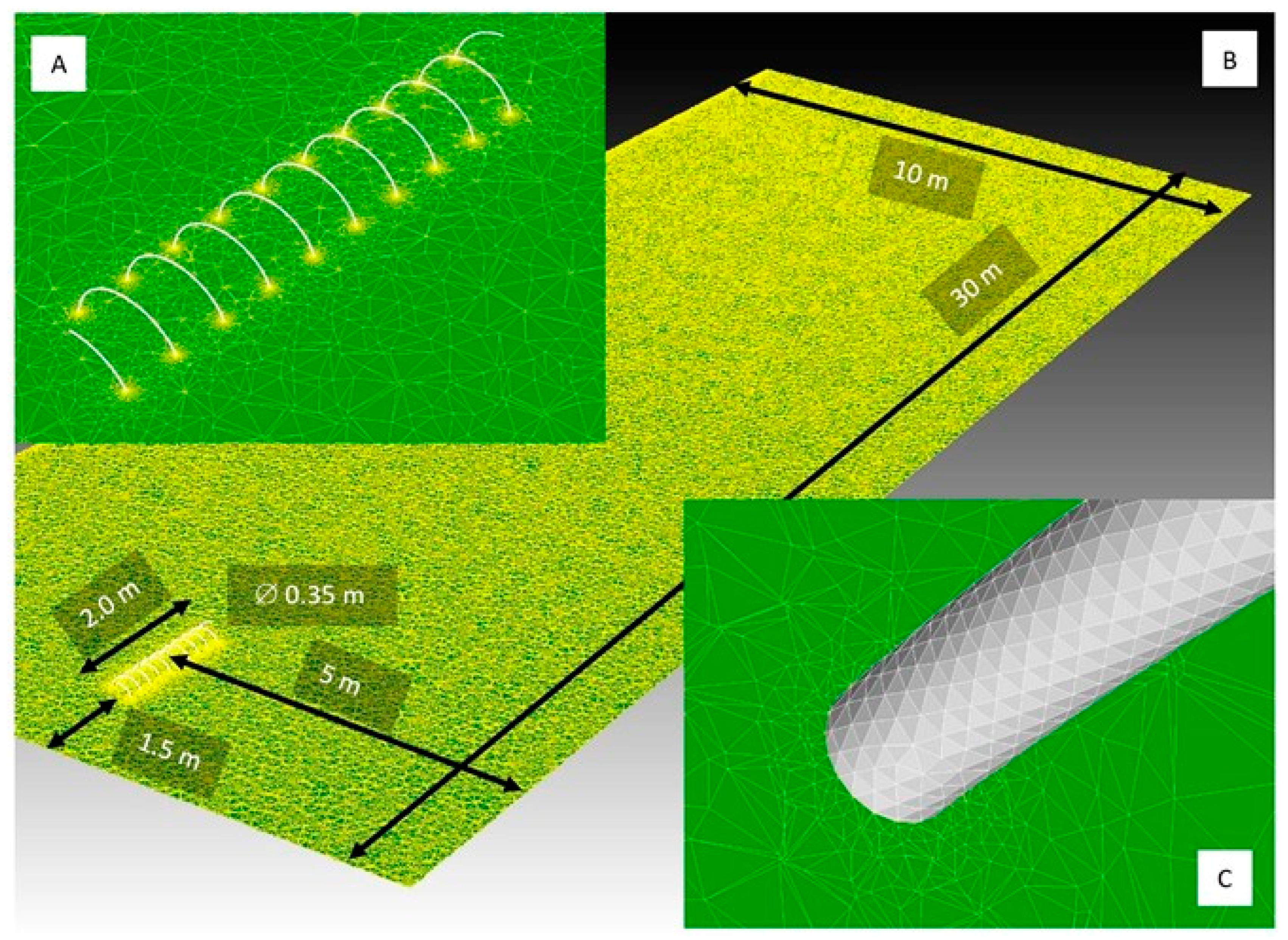Mesh generation followed the strategy presented previously [13,20,21]. The surface was meshed with triangles with a cell side length of 8.6 mm and a successive grading was introduced to reach a maximum cell size of 12.6 million triangles, producing an unstructured mesh with a cell side length of approximately 10 cm on the outer boundaries. In the simulations presented there, a geometrical match between the experiment and simulations had to be achieved. Furthermore, the temperature at the four sides and the bottom was fixed to a value of 10 °C. This is not realistic in free field applications and not possible in the FLS methodology. Therefore, the computational domain was increased significantly to a volume of 10 m × 10 m × 30 m = 3000 m³ and meshed with 12.65 million cells.

Table 1. Overview of soil thermal parameters and earth basket spiral heat exchanger dimensions used for the validation [14].

Parameter	Value
Soil thermal conductivity (W/mK)	1.0	1.5		2.0
Soil heat capacity (J/kgK)	2500
Soil density (kg/m3)	1000
Soil temperature (°C)	10.0
Buried depth (m)	1.5
Ring diameter (m)	0.35
Pipe outer diameter (m)	0.06
Number of rings	10
Total pipe length (m)	11.04
Total heat exchanger length (m)	2.0
Pitch (m)	0.2
Specific heat injection rate (W/m)	5	10	15	25

summarizes the earth basket spiral heat exchanger dimensions and the material parameters used throughout both the CFD and FLS simulations.

An important boundary condition for validation is the heat injection rate. The heat injection rates considered (ranging between 5 and 25 W/m, Table 1) were deemed realistic for a spiral ground heat exchanger/earth basket heat exchanger as they are generally used in practice. As an example, in a practical application, an earth basket heat exchanger with a diameter of 1.4 m and an active depth of 4 m with a pitch of 0.25 m (length 70 m) and 25 W/m maximum load would support a capacity of 1.8 kW.

The experiment used to validate the CFD procedure was described in [13]. It is based on an earth basket heat exchanger modelled with an electric heating cable to provide constant heat flux, which was installed in the form of a spiral-shaped heat exchanger in a container. To guarantee constant boundary conditions, the measurements were carried out in a climate chamber at a defined ambient temperature. A plastic grid net acted as a support structure for the geometry of the heating cable. In the box, several temperature sensors and a DTS (distributed temperature sensing) system were installed. Finally, the box was filled with soil. A comparison between CFD and the experiment was reported in [20].

In Figure 2, the dimensions of the computational domain and earth basket spiral heat exchanger are given, together with images of the computational mesh in 3 grades of detail (B: overview, A: detail of the full slinky and C: detail of one ring of the slinky).

In this application, the Navier Stokes solver was used only for solving the energy equation using a second-order upwind scheme. When applicable, a first-order implicit transient formulation was employed. Six different sets of boundary conditions were applied to the same geometry with variations in the specific heat injection rate and the conductivity (See

Table 2. Boundary conditions (CFD/FLS).

Specific Heat Injection Rate (W/m) 1	CFD Heat Flux (W/m2)	Surface Area (m2)	Heat Injection Rate (W)
5	269.63	0.208151	56.123
10	539.25	0.208151	112.245
15	808.88	0.208151	168.369
25	1348.125	0.208151	280.613

¹ Corresponding length of FLS helix is 11.04 m.

). For the CFD simulations, calculations with two different time step sizes of Dt = 90 s and Dt = 900 s were performed with 50 iterations per timestep. This was accompanied by a solution with a steady formulation of the energy equation Dt = ∞ s. For all cases, the temperature was initialized with a value of 283.15 K (corresponding to 10 °C) everywhere. At the six boundary walls of the cube, a temperature boundary condition of 283.15 K was set. The surface of the earth basket spiral heat exchanger was set to a heat flux boundary condition, fixing the heat flux to the values in column 2 of Table 2.

3. Results

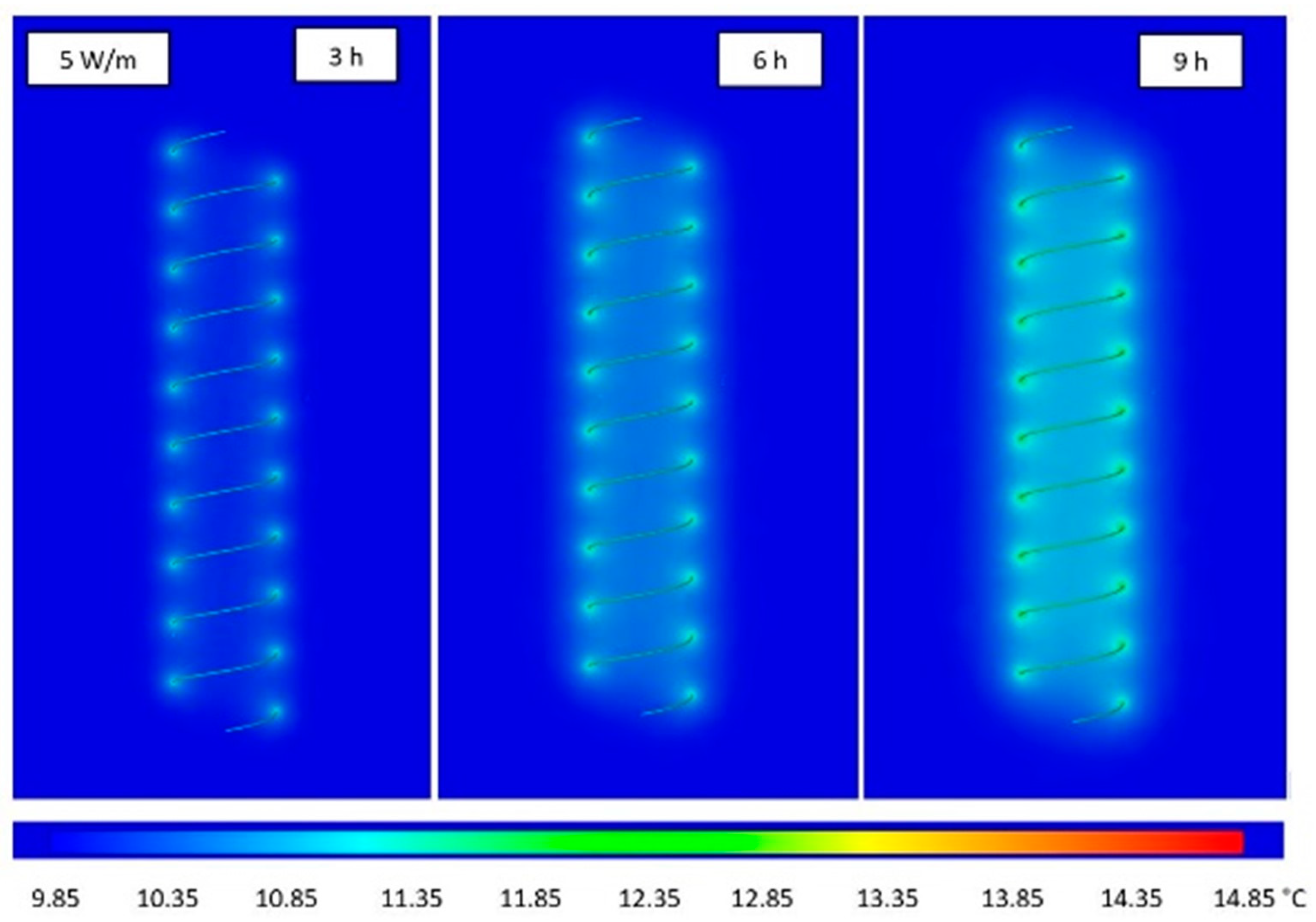
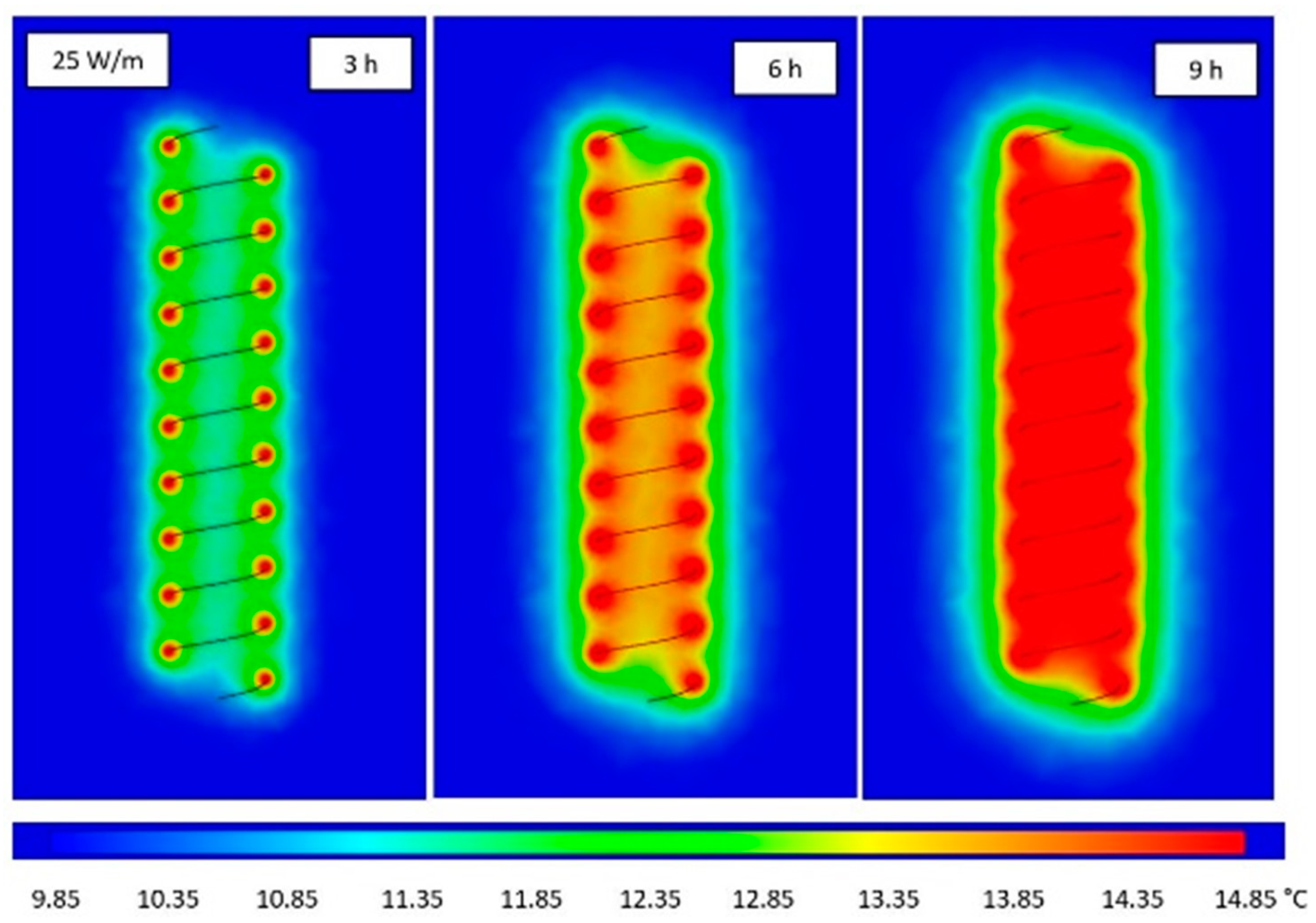
For the visualization of the resulting temperature field on a vertical plane through the earth basket spiral heat exchanger and the surface temperature on the helix rings, Figure 3 and Figure 4 show the evolution for three different times (3 h, 6 h and 9 h). In Figure 3, the specific heat injection rate was set to 5 W/m and the results presented in Figure 4 correspond to a specific heat injection rate of 25 W/m. The colour gradient was set to the same values in Figure 3 and Figure 4. Here, only the results of CFD calculations are shown. For the transient case, the calculation times for FLS would be prohibitive because each point in the plane would have to be calculated separately.

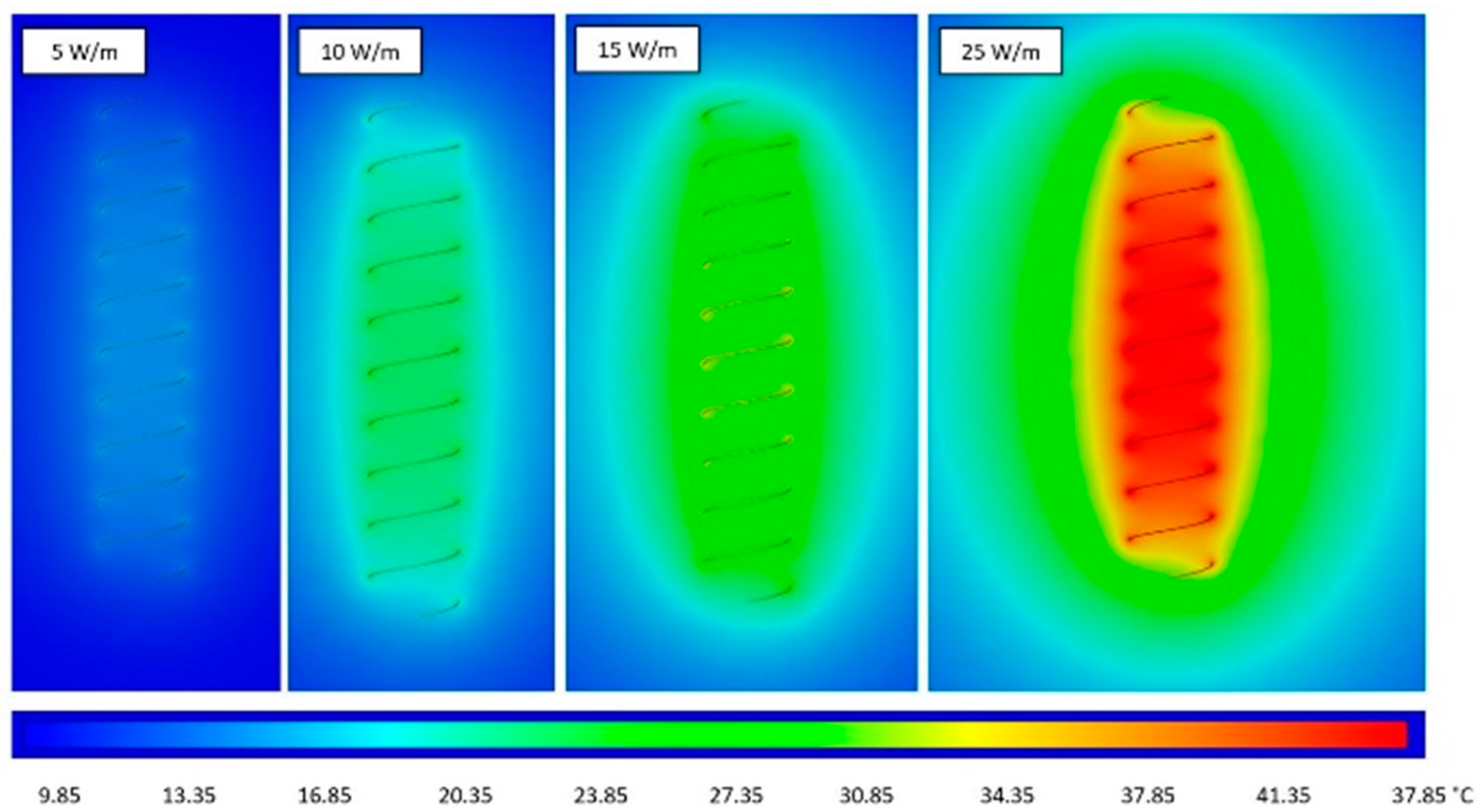
The results for the steady-state solution are given for specific heat injection rates of 5, 10, 15 and 25 W/m in Figure 5. The colour gradient was changed in comparison with Figure 3 and Figure 4 to allow for the presentation of significantly higher temperatures for longer times. The FLS data would again need a calculation on all points on the planes.

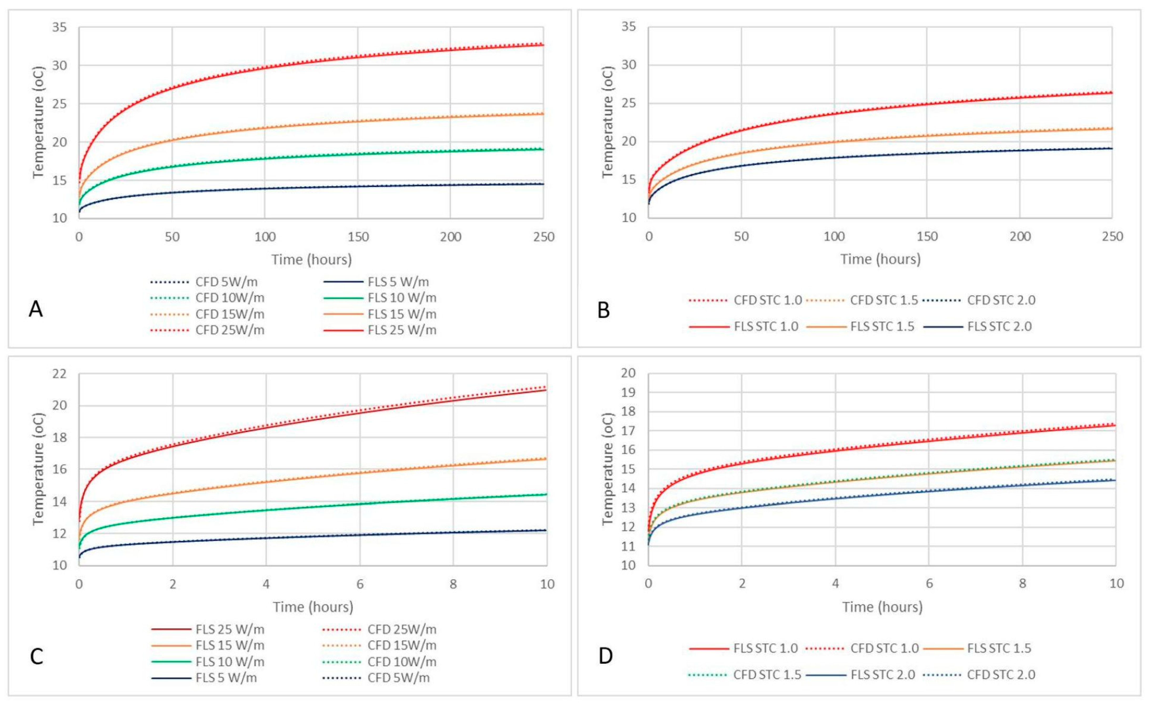
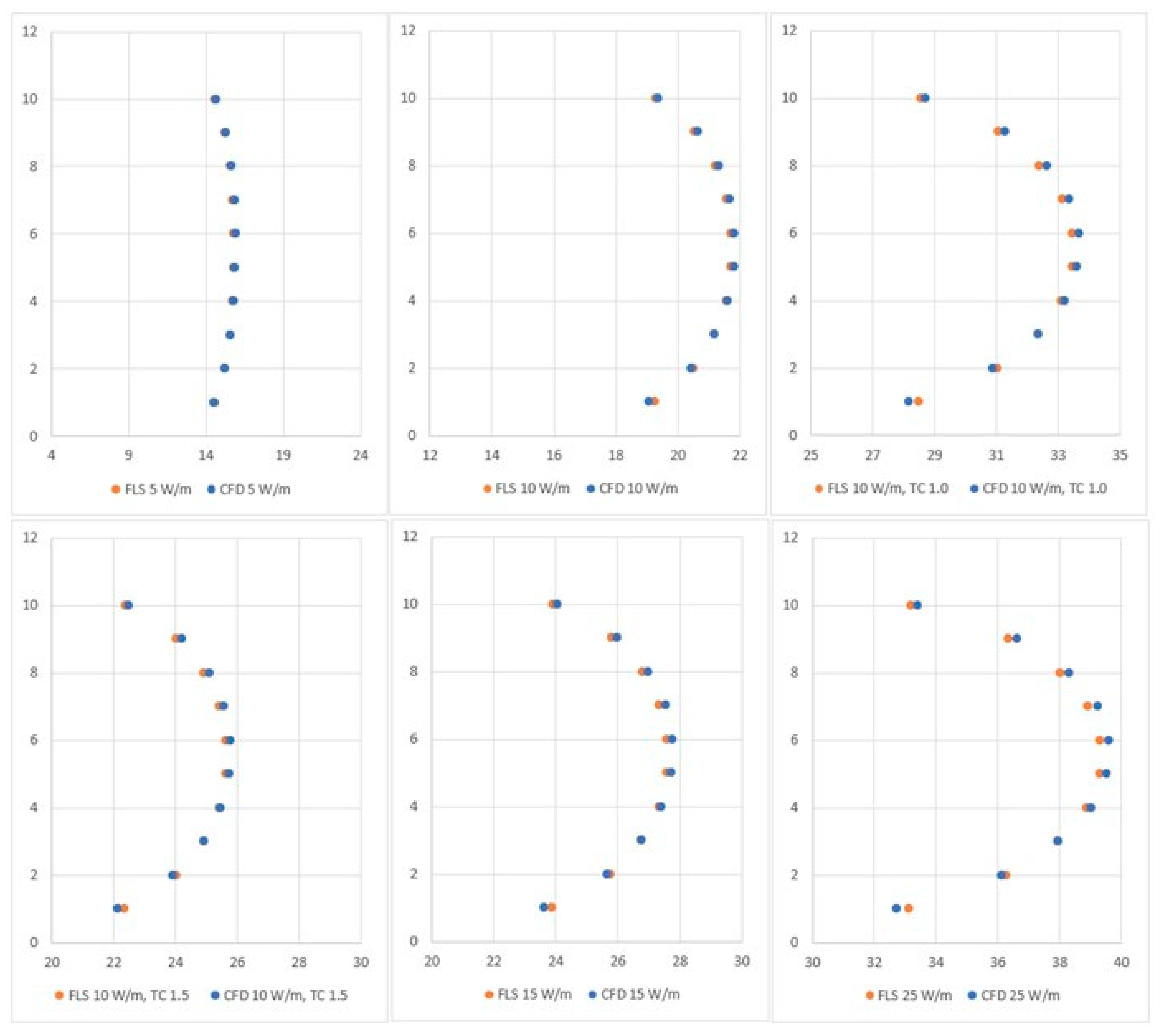
Figure 6 compares the CFD and FLS results for the six sets of boundary conditions both for long-term behaviour (A and B) and short-term behaviour (C and D). The left figures show a comparison of different specific heat injection rates and the right figures show a comparison for different thermal conductivities of the soil.

Table A1. Short-term transient results for the surface temperature of the earth basket spiral heat exchanger for different specific heat injection rates.

t (h)	5 W/m		10 W/m		15 W/m		25 W/m
	CFD	FLS	CFD	FLS	CFD	FLS	CFD	FLS
0	10.00	10.00	10.00	10.00	10.00	10.00	10.00	10.00
1	11.34	11.32	12.68	12.64	14.02	13.97	16.69	16.58
2	11.51	11.49	13.02	12.98	14.53	14.47	17.55	17.42
3	11.64	11.62	13.28	13.23	14.91	14.85	18.19	18.05
4	11.75	11.73	13.50	13.45	15.25	15.18	18.74	18.60
5	11.85	11.82	13.70	13.65	15.54	15.47	19.24	19.08
6	11.94	11.91	13.88	13.83	15.81	15.74	19.69	19.52
7	12.02	11.99	14.04	13.99	16.06	15.98	20.10	19.93
8	12.10	12.07	14.19	14.14	16.29	16.21	20.48	20.31
9	12.17	12.14	14.33	14.28	16.50	16.42	20.84	20.65
10	12.23	12.21	14.47	14.41	16.70	16.62	21.17	20.98

,

Table A2. Short-term transient results for the surface temperature of the earth basket spiral heat exchanger for a specific heat injection rate of 10 W/m and different soil thermal conductivities.

t (h)	1.0 W/(mK)		1.5 W/(mK)		2.0 W/(mK)
	CFD	FLS	CFD	FLS	CFD	FLS
0	10.00	10.00	10.00	10.00	10.00	10.00
1	14.78	14.71	13.41	13.36	12.68	12.64
2	15.36	15.29	13.82	13.77	13.02	12.98
3	15.73	15.66	14.12	14.06	13.28	13.23
4	16.04	15.96	14.37	14.31	13.50	13.45
5	16.31	16.23	14.59	14.53	13.70	13.65
6	16.55	16.47	14.80	14.74	13.88	13.83
7	16.78	16.69	14.99	14.93	14.04	13.99
8	17.00	16.91	15.17	15.10	14.19	14.14
9	17.20	17.11	15.33	15.27	14.33	14.28
10	17.39	17.30	15.49	15.42	14.47	14.41

,

Table A3. Long-term transient results for the surface temperature of the earth basket spiral heat exchanger for different specific heat injection rates.

t (h)	5 W/m		10 W/m		15 W/m		25 W/m
	CFD	FLS	CFD	FLS	CFD	FLS	CFD	FLS
0	10.00	10.00	10.00	10.00	10.00	10.00	10.00	10.00
50	13.44	13.38	16.87	16.79	20.31	20.18	27.18	26.97
100	13.97	13.90	17.94	17.84	21.91	21.76	29.85	29.60
150	14.26	14.19	18.52	18.41	22.77	22.62	31.29	31.03
200	14.45	14.37	18.90	18.79	23.34	23.18	32.24	31.96
250	14.59	14.51	19.17	19.06	23.76	23.58	32.93	32.64
∞ 1	15.45	15.35	20.90	20.74	26.35	26.11	37.25	36.85

¹ steady-state calculation for CFD, semi-infinite calculation for FLS.

and

Table A4. Long-term transient results for the surface temperature of the earth basket spiral heat exchanger for a specific heat injection rate of 10 W/m and different soil thermal conductivities.

t (h)	1.0 W/(mK)		1.5 W/(mK)		2.0 W/(mK)
	CFD	FLS	CFD	FLS	CFD	FLS
0	10.00	10.00	10.00	10.00	10.00	10.00
50	21.56	21.42	18.55	18.45	16.87	16.79
100	23.74	23.57	20.01	19.88	17.94	17.84
150	25.01	24.82	20.82	20.68	18.52	18.41
200	25.88	25.68	21.36	21.22	18.90	18.79
250	26.53	26.32	21.75	21.61	19.17	19.06
∞ 1	31.79	31.34	24.53	24.32	20.90	20.74

¹ steady-state calculation for CFD, semi-infinite calculation for FLS (corresponding to 100,000 h).

in Appendix A list the surface temperature values for both the FLS and CFD results for the first 10 h and every 50 h up to 250 h, including the result for the steady state.

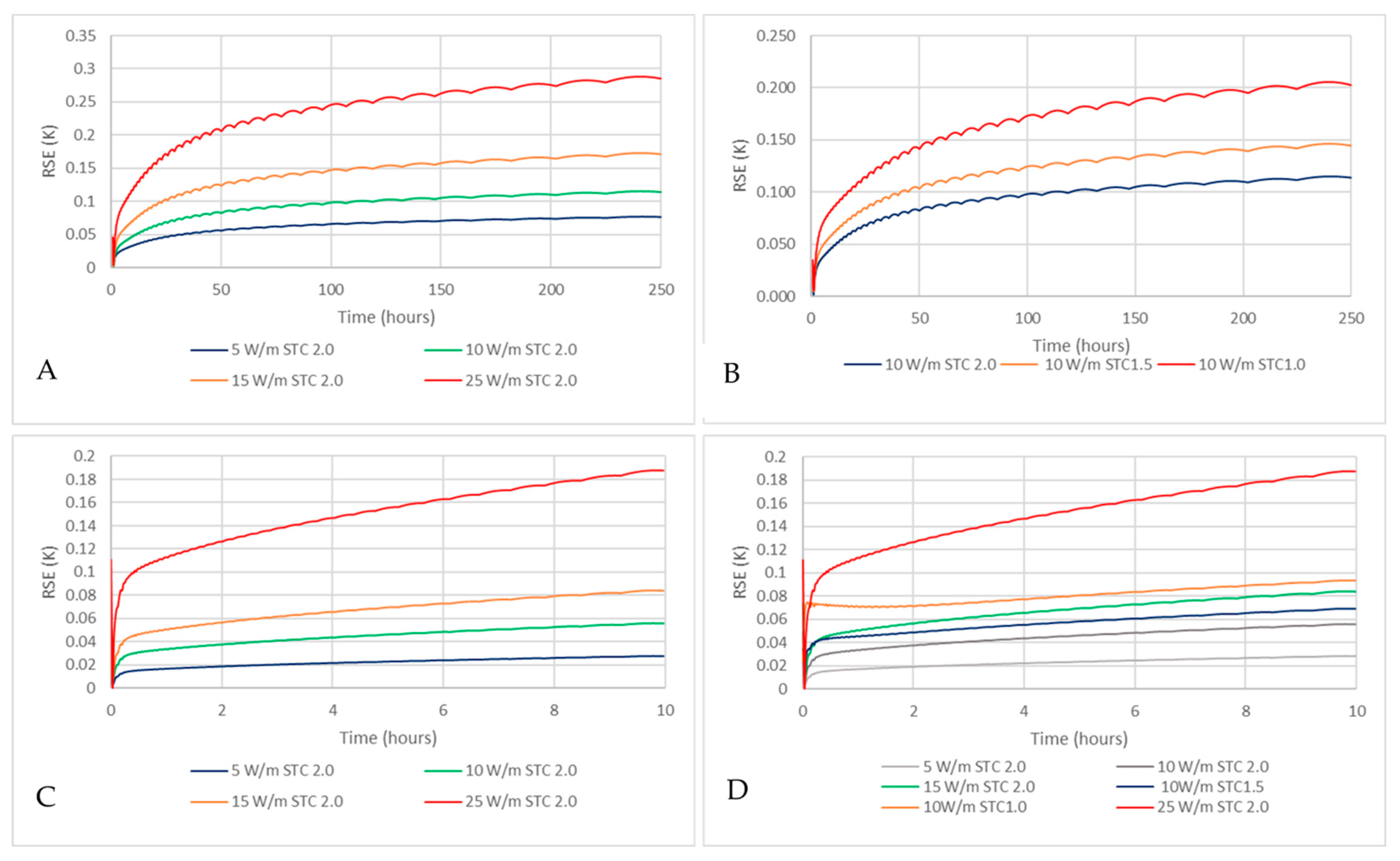
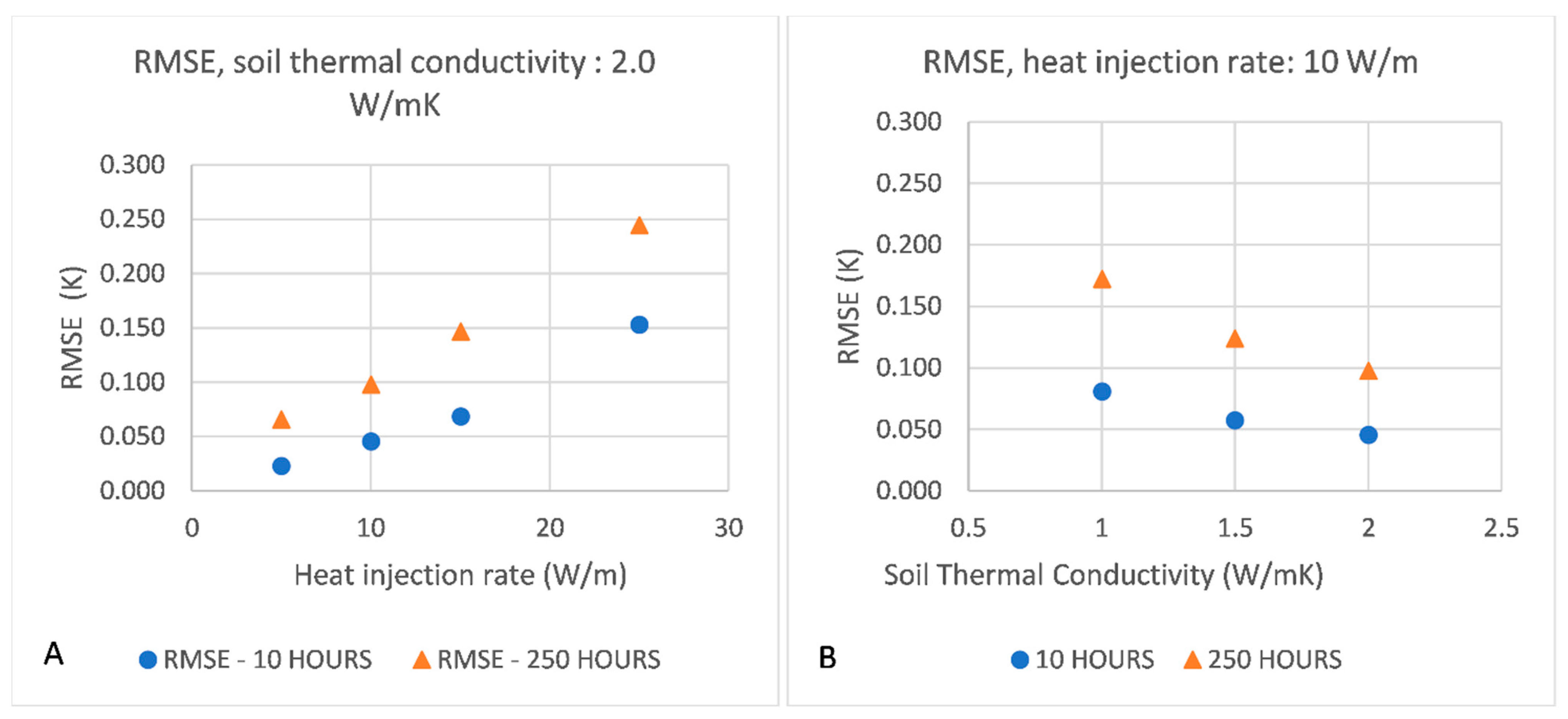
As a measure of the fit between the CFD and FLS models, the root-square-error (RSE) value was calculated and is shown in Figure 7 again for long- and short-term behaviour at specific heat injection rates (left side) and soil conductivities (right side). The root-square-error for the long-term simulation with a larger timestep was smaller than 0.3 K, even for the highest injection rate; for the shorter simulation with a timestep of 90 s, the RSE was smaller than 0.2 K. When the soil thermal conductivity was changed, the RSE was, in all cases, smaller than 0.21 K.

Some oscillations were apparent in the RSE; close examination of the data series revealed that these oscillations occurred in the FLS solution. As the error introduced was less than ±0.025 K, this did not significantly affect the results.

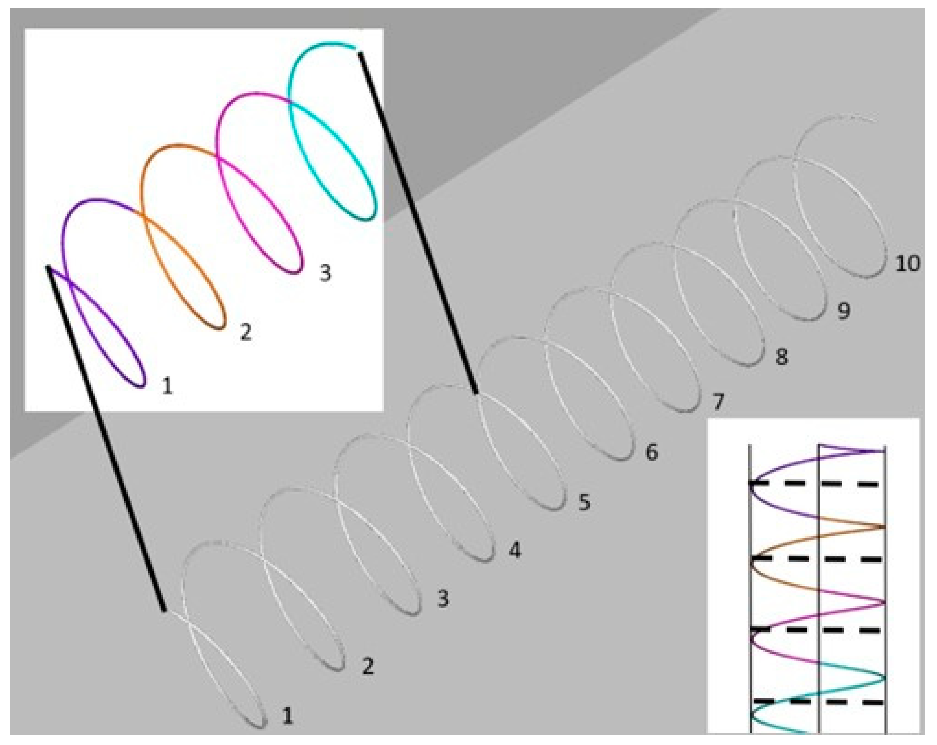
As discussed before, the ten rings considered for this earth basket heat exchanger were modelled differently in CFD and FLS. In the FLS, the spiral heat exchanger was modelled as a stack of discrete rings, whereas in CFD, the full twisted geometry was realized. Figure 8 shows the earth basket heat exchanger and the different parts of the CFD geometry, which were attributed to the single rings in FLS.

For the different sets of boundary conditions presented above, temperatures were evaluated on the 10 different sections of the CFD earth basket heat exchanger and compared with the results of the FLS. This comparison was performed for the steady-state solution as it was not practical to compute the individual ring solutions for transient simulation (see Figure 9). Overall, there was good correspondence with the solutions for the individual rings between the FLS and CFD. The difference between FLS and CFD was about 0.4 K, showing an average error over all rings of 0.06 K–0.23 K.

4. Discussion

As the main purpose of this paper was to validate the proposed FLS approach by a full-geometry-resolved three-dimensional solution of the differential equation of energy, the time-resolved curves shown in Figure 9 were condensed to error values for two different times (10 and 250 h) and are shown for the six boundary condition variations in Figure 10. The left side shows the root-mean-square error (RMSE) for the four different specific heat injection6 rates, resulting in a maximum RMSE value of 0.245 K for a duration of 250 h and a specific heat injection rate of 25 W/m. When changing the thermal conductivity of the soil from 2.0 to 1.0 W/mK, the maximum RMSE was 0.172 K for a soil thermal conductivity of 1.0 W/mK and a specific heat injection rate of 10 W/m. The corresponding numerical values are given in

Table 3. Root-mean-square error between the CFD and FLS results for the surface temperature of the earth basket spiral heat exchanger (based on short-term transient results).

Specific Heat Injection Rate (W/m)	Therm. Conductivity W/(mK)	RMS Error K	Relative RMS Error K/(W/m)
5	2.0	0.023	0.0046
10	1.0	0.081	0.0081
	1.5	0.057	0.0057
	2.0	0.046	0.0046
15	2.0	0.069	0.0046
25		0.153	0.00612

for the short-term behaviour and in

Table 4. Root-mean-square error between the CFD and FLS results for the surface temperature of the earth basket spiral heat exchanger (based on long-term transient results).

Specific Heat Injection Rate (W/m)	Therm. Conductivity W/(mK)	RMS Error K	Relative RMS Error K/(W/m)
5	2.0	0.066	0.0132
10	1.0	0.172	0.0172
	1.5	0.124	0.0124
	2.0	0.098	0.0098
15	2.0	0.147	0.0098
25		0.245	0.0098

for the long-term behaviour. We have shown, in this paper, that the combination of a FLS with a G-function is suitable for accurate and fast design calculations for complex ground heat exchanger topologies.

5. Summary and Conclusions

In this paper, we present a comparison between the transient response of a detailed numerical computational fluid dynamics model and a new analytical model based on the well-known finite line source solution for spiral (earth basket) ground heat exchangers.

The results show a very good agreement between the two models for a realistic range of boundary conditions, such as the specific heat injection rate and soil thermal conductivity. The root-mean-square error (RMSE), a measure of fit between the CFD and FLS models, was, in the worst case, still less than 0.25 K.

In a previous study [14], the steady-state behaviour of the CFD and FLS models was evaluated for a range of specific heat injection rates, soil thermal conductivities and different geometries (variation in spiral diameter and pitch). Those results also showed a very good agreement between the CFD and FLS approaches.

Therefore, the final conclusion is that, despite the several simplifying assumptions made for the analytical FLS model, the approach is more than sufficiently accurate to be used in engineering and design software for these types of ground heat exchangers in the very long term (30 years of operation or more), long term (250 h range) and in the short term (minutes to hours) when used for heat pump cycle (peak load) analysis.

References

1. Eskilson, P. Thermal Analysis of Heat Extraction Boreholes. Ph.D. Thesis, Lund University, Department of Mathematical Physics, Lund, Sweden, 1987. [Google Scholar]
2. Spitler, J.D.; Bernier, M. Vertical borehole heat exchanger design methods. In Advances in Ground-Source Heat Pump Systems; Woodhead Publishing: Duxford/Kidlington, UK; Cambridge, MA, USA, 2016. [Google Scholar]
3. Spitler, J.D. GLHEPRO—A Design Tool for Commercial Building Ground Loop Heat Exchangers. In Proceedings of the Fourth International Heat Pumps in Cold Climates Conference, Québec, ON, Canada, 17–18 August 2000. [Google Scholar]
4. Xiong, Z.; Fisher, D.E.; Spitler, D. Development and validation of a Slinkytm ground heat exchanger model. Appl. Energy 2015, 141, 57–59. [Google Scholar] [CrossRef]
5. Cui, P.; Li, X.; Man, Y.; Fang, Z. Heat transfer analysis of pile geothermal heat exchangers with spiral coils. Appl. Energy 2011, 88, 4133–4139. [Google Scholar] [CrossRef]
6. Li, H.; Nagano, K.; Lai, Y. A new model and solutions for a spiral heat exchanger and its experimental validation. Int. J. Heat. Mass. Transf. 2012, 55, 4404–4414. [Google Scholar] [CrossRef]
7. Wang, D.; Lu, L.; Cui, P. A new analytical solution for horizontal geothermal heat exchangers with vertical spiral coils. Int. J. Heat. Mass. Transf. 2016, 100, 111–120. [Google Scholar] [CrossRef]
8. GEOFIT Project. 2018. Available online: https://geofit-project.eu/ (accessed on 10 April 2022).
9. Meeng, C.L. Development of an Engineering Tool for the Design of Novel Shallow Ground Heat Exchangers—GEOFIT. Master’s Thesis, Technical University of Eindhoven, Eindhoven, The Netherland, 2020. [Google Scholar]
10. Cimmino, M.; Bernier, M.; Adams, F. A contribution towards the determination of g-functions using the finite line source. Appl. Therm. Eng. 2013, 51, 401–413. [Google Scholar] [CrossRef]
11. Blomberg, T.; Claesson, J.; Eskilson, P.; Hëllström, G.; Sanner, B. Earth Energy Designer—EED, Version 4.20; BLOCON: Lund, Sweden, 2019. [Google Scholar]
12. Kling, S.; Haslinger, E.; Lauermann, M.; Witte, H.J.L.; Reichl, C.; Steurer, A.; Dörr, C.; Dragisa, P.; Robin, F. Geofit: Experimental investigations and numerical validation of shallow spiral collectors as a bases for development of a design tool for geothermal retrofitting of existing buildings. In Proceedings of the European Geothermal Congress 2022, Berlin, Germany, 17–21 October 2022. [Google Scholar]
13. Kling, S.; Haslinger, E.; Lauermann, M.; Witte, H.; Reichl, C.; Steurer, A.; Dörr, C. Design Framework and Laboratory Experiments for Helix and Slinky Type Ground Source Heat Exchangers for Retrofitting Projects. Processes 2022, 10, 959. [Google Scholar] [CrossRef]
14. Witte, H.J.L.; Heinrichs, F.A.; Reichl, C.; Meeng, C.M.; Doerr, C.; Steurer, A.; Kling, S. Development and validation of analytical solutions for earth basket (spiral) heat exchangers. In Proceedings of the European Geothermal Congress 2022, Berlin, Germany, 17–21 October 2022. [Google Scholar]
15. Man, Y.; Yang, H.; Dao, N.; Cji, P.; Liu, L.; Fang, Z. Development of spiral heat source model for novel pile ground heat exchangers. HVAC R Res. 2011, 17, 1075–1088. [Google Scholar]
16. Lei, F.; Hu, P.; Huang, X. Hybrid analytical model for composite heat transfer in spiral pile ground heat exchanger. Appl. Thermal Eng. 2018, 137, 555–566. [Google Scholar] [CrossRef]
17. Kim, M.J.; Lee, S.R.; Yoon, S.; Jeon, J.S. Evaluation of geometric factors influencing thermal performance of horizontal sprial-coil ground heat exchangers. Appl. Therm. Eng. 2018, 144, 788–796. [Google Scholar] [CrossRef]
18. Conti, P. An analytical method to simulate the dynamic performances of truncated cone helix ground heat exchangers. In Proceedings of the 73rd Conference of the Italian Thermal Machines Engineering Association, Pisa, Italy, 12–14 September 2018. [Google Scholar]
19. Beyzan, B.; Porkhial, S.; Aboui, M.A. 3-D simulation of heat transfer rate in geothermal pile-foundation heat exchangers with spiral pipe configuration. Appl. Therm. Eng. 2015, 87, 655–668. [Google Scholar] [CrossRef]
20. Steurer, A. Numerical CFD Simulation of Geothermal Heat Exchangers. Master Thesis, Montanuniversität Leoben, Leoben, Austria, 2021. Available online: https://pure.unileoben.ac.at/portal/files/7819388/AC16360870.pdf (accessed on 25 April 2023).
21. Dörr, C. CFD Analysis of Ground Source Heat Exchangers. Master Thesis, Montanuniversität Leoben, Leoben, Austria, 2020. Available online: https://pure.unileoben.ac.at/portal/files/6087346/AC16129131.pdf (accessed on 25 April 2023).
Figure 1. Installation of a spiral (earth basket) ground heat exchanger with a fibre-optic distributed temperature sensing system at the IUT Civil Engineering Student Laboratory (Bordeaux, France) pilot site (picture: Groenholland Geo Energy systems).
Processes 11 01418 g001
Figure 2. Geometry and mesh for CFD calculations shown in 3 grades of detail ((B): overview, (A): detail of full slinky and (C): detail of one ring of the slinky).
Processes 11 01418 g002
Figure 3. Surface temperature on the earth basket spiral heat exchanger surface and a vertical central plane for a specific heat injection rate of 5 W/m after 3, 6 and 9 h.
Processes 11 01418 g003
Figure 4. Surface temperature of the earth basket spiral heat exchanger and a vertical central plane for a specific heat injection rate of 25 W/m after 3, 6 and 9 h.
Processes 11 01418 g004
Figure 5. Surface temperature on the earth basket spiral heat exchanger surface and the vertical central plane of the steady state solution for specific heat injection rates of 5, 10, 15 and 25 W/m.
Processes 11 01418 g005
Figure 6. Temperature evolution calculated with CFD (dotted lines) and FLS solutions (continuous lines) for 250 h 900 s timestep simulations (top graphs) and 10 h 90 s time step detailed simulations (bottom graphs). (A): 250 h 900 s timestep with different heat injection rates (soil thermal conductivity 2.0 W/mK); (B): 250 h 900 s timestep with 10 W/m heat injection rate and different soil thermal conductivities. (C): 10 h 90 s timestep with different heat injection rates (soil thermal conductivity 2.0 W/mK); (D): 10 h 90 s timestep with 10 W/m heat injection rate and different soil thermal conductivities.
Processes 11 01418 g006
Figure 7. Root-square-error between CFD and FLS solutions for 250 h 900 s timestep simulations (top graphs) and 10 h 90 s time step detailed simulations (bottom graphs). (A): 250 h 900 s timestep with different specific heat injection rates (soil thermal conductivity 2.0 W/mK); (B): 250 h 900 s timestep with 10 W/m specific heat injection rate and different soil thermal conductivities. (C): 10 h 90 s timestep with different specific heat injection rates (soil thermal conductivity 2.0 W/mK); (D): 10 h 90 s timestep with 10 W/m heat injection rate and different soil thermal conductivities.
Processes 11 01418 g007
Figure 8. CFD geometry of an earth basket heat exchanger colouring the 10 different parts that were modelled as horizontal rings in the FLS. The top-left insert shows 4 parts that were used for evaluation to compare with FLS. The bottom-right insert shows the position of the FLS rings (dashed lines) in comparison with the CFD model.
Processes 11 01418 g008
Figure 9. Ring-by-ring (local) comparison of temperatures for the different sets of boundary conditions. Temperature is shown on the x-axis and is arranged such that the ranges of 20 K are equal for all figures. The ring number is shown on the y-axis ranging from 1 to 10.
Processes 11 01418 g009
Figure 10. (A): Root-mean-square error (RMSE) at different specific heat injection rates for a 10 h 90 s timestep and a 250 h 900 s timestep. Soil thermal conductivity: 2.0 W/mK. (B): Root-mean-square error at different soil thermal conductivities for a 10 h 90 s timestep and a 250 h 900 s timestep; specific heat injection rate: 10 W/m.
Processes 11 01418 g010