Article

Hyperparameter Search for Machine Learning Algorithms for Optimizing the Computational Complexity

1
Department of Information Systems, College of Computer and Information Sciences, King Saud University, P.O. Box 51178, Riyadh 11543, Kingdom of Saudi Arabia (KSA)
2
Electrical Engineering Department, College of Engineering, King Saud University, P.O. Box 800, Riyadh 11421, Kingdom of Saudi Arabia (KSA)
3
Department of Software Engineering, College of Computer and Information Sciences, King Saud University, P.O. Box 22452, Riyadh 11495, Kingdom of Saudi Arabia (KSA)
*
Authors to whom correspondence should be addressed.
Processes 2023, 11(2), 349; https://doi.org/10.3390/pr11020349
Submission received: 13 December 2022 / Revised: 17 January 2023 / Accepted: 17 January 2023 / Published: 21 January 2023
(This article belongs to the Special Issue Evolutionary Process for Engineering Optimization (II))

Abstract

:
For machine learning algorithms, fine-tuning hyperparameters is a computational challenge due to the large size of the problem space. An efficient strategy for adjusting hyperparameters can be established with the use of the greedy search and Swarm intelligence algorithms. The Random Search and Grid Search optimization techniques show promise and efficiency for this task. The small population of solutions used at the outset, and the costly goal functions used by these searches, can lead to slow convergence or execution time in some cases. In this research, we propose using the machine learning model known as Support Vector Machine and optimizing it using four distinct algorithms—the Ant Bee Colony Algorithm, the Genetic Algorithm, the Whale Optimization, and the Particle Swarm Optimization—to evaluate the computational cost of SVM after hyper-tuning. Computational complexity comparisons of these optimization algorithms were performed to determine the most effective strategies for hyperparameter tuning. It was found that the Genetic Algorithm had a lower temporal complexity than other algorithms.

1. Introduction

Hyperparameters of machine learning algorithms are notoriously hard to modify without a lot of computational work [1]. An effective strategy for adjusting hyperparameter values can be developed with the help of the greedy search and swarm intelligence algorithms. To this end, optimization strategies based on random searches and grid searches have proven to be both effective and promising. Convergence or running time may be slowed down due to the costly objective functions used by these searches and the small population of initial answers [2].
A learning algorithm’s hyperparameters are the parameters whose values regulate the learning process and determine the models’ final parameters. Finding the best settings for hyperparameters to get good results from data as quickly as possible is the purpose of hyperparameter optimization [3]. Any machine learning system will only be as good as its training phase. Machine learning relies on algorithms that can adapt to new situations and boost their own efficiency over time. These parameters of the model were discussed in [4].
However, some parameters cannot be adjusted during training and must be set up ahead of time. The common term for these adjustments is “hyperparameters”. Data transformation parameters and model structure hyperparameters are defined in [5].
Changes to a machine learning model’s hyperparameters can have a significant impact on the model’s predictive performance. A high value for the “tree depth” hyperparameter can reduce the efficiency of the decision tree method [6]. This shows how careful work with hyperparameters is essential. There are a variety of methods for finding the optimal hyperparameters for a specific data collection [7]. When it comes to precision, a manual setting has its advantages. This allows checks that the selected hyperparameter values are having the expected effect by re-evaluating the model after each iteration. Manually adjusting each hyperparameter requires a lot of time and trial and error [8].
Recommended hyperparameter settings in the software package are typically based on prior research and experience; therefore, this is another way to find a good hyperparameter setup. Even though the default settings produce satisfactory results on a test dataset, they may not yield the optimum overall accuracy. Methods for optimizing hyperparameters are also an option. These techniques are optimization algorithms that make use of the data at hand to lessen the generalization error of the machine learning model for any given set of hyperparameters [9].
The effect of the default settings of hyperparameters on the performance of ML algorithms has been studied [10], and the results have been compared to those obtained by employing various hyperparameter-tweaking techniques. Most studies investigate various ways for optimizing hyperparameters in machine language tools in order to address a particular classification issue. The characteristics of the problem strongly affect the classification accuracy of a machine learning technique and the optimal combination of hyperparameters for optimum classification accuracy [11,12].
The current article’s originality lies in the rigorous testing of machine learning methodologies, the broad comparison of hyperparameter tuning algorithms, and the originality of the classification problem itself. No previous study has used hyperparameter tuning methods to identify which values for these hyperparameters would result in the maximum classification accuracy for the particular machine learning algorithm being used. It is important to note that the values for these hyperparameters will vary depending on the classification task at hand. The main objective of this research is:
(a)
To use different ML-based datasets to test the multiple optimization approaches.
(b)
To design hybrid Hyperparameter models for testing the computational time, accuracy and cost of proposed model.

2. Related Work

Machine learning models are used frequently [13]. Hyperparameters can increase a classifier’s performance. Grid Search, Random Search, Bayesian Optimization, PSO, and the Genetic Algorithm have been compared (GA). Logistic Regression (LR), Ridge Classifier (RC), SVC, DT, and NB improve six machine learning algorithms (NB). Change Arabic sentiment data tests hyperparameters. Sentiment analysis identifies positive and negative emotions. Arabic’s morphology makes meaning inferences difficult. All classifiers are evaluated on this dataset after hyperparameter tuning. Each hyperparameter-adjustment method has been discussed. The before-and-after score for SVC’s hyperparameter was 95.6208.
The authors of [8] improved ML hyperparameters. Machine learning algorithms were updated using cutting-edge optimization methodologies. This paper answered several hyperparameter optimization questions. Benchmark datasets showed optimization methodologies and hyperparameter tuning. Optimizations of this poll helps industrial users, data analysts, and researchers identify machine learning hyperparameters. Hyperparameter tweaking is computationally demanding [12]. Swarm intelligence can tune hyperparameters. ABC has such potential. If ABC has few solutions and an expensive objective function, convergence and execution time may be slow. OptABC speeds up the ABC algorithm’s near-optimal solution search. OptABC blends bee-inspired techniques with K-means clustering, greedy algorithms, and opposition-based learning. These tactics allow OptABC to expand the training set and speed convergence without losing accuracy. Comparing this strategy to others tests its validity. Experimentally, OptABC outperforms best practises.
NLP and ML have tricky hyperparameter tweaking. Sequential Bayesian Optimization reduces iterations and trials by using previous information. Our paper describes multi-stage hyperparameter optimization with more data. First, candidates’ speed and performance were quickly assessed. Researchers have linked this novel method to Bayesian Optimization [10]. Machine learning solves problems. Different conditions need adjusting ML model hyperparameters [14]. Hyperparameters impact ML model performance. Machine learning and hyperparameter optimization are required. Autonomous optimization strategies have pros and cons. Our study changed machine learning hyperparameters to boost performance, and discusses machine learning optimization. We address issues in hyperparameter optimization research and review tools and frameworks. Benchmark datasets examine optimization methodologies and illustrate hyperparameter adjustment. Hyperparameter tuning for machine learning models benefits industrial users, data analysts, and researchers.
Optimizing hyperparameters uses grid and manual searches. Random trials are superior to grid trials for optimizing hyperparameters [7]. Empirical evidence supports grid search and manual search for deep-belief neural networks. Randomly searching the same topic can find better or equal models. Random search delivers better model results by searching a larger, less attractive configuration space. Manual and grid search produces deep belief networks that have outperformed less thorough alternatives on four of seven datasets. Gaussian process analysis considers just data-set-based hyperparameters. Grid search doesn’t work well with new data sets. Recent “High Throughput” algorithms examine many hyperparameters to get good results. Increasing interest in large hierarchical models involves comparing adaptive (sequential) hyperparameter optimization algorithms to random search, as random search provides a natural baseline against which progress may be measured.
Modern supervised machine learning requires hyperparameters. Optimize prediction outcomes by using the software’s default variables, explicitly configuring them, or adjusting. Two goals drive this investigation. Researchers provide ways to assess algorithmic hyperparameter tunability and data-based defaults. Six machine-learning algorithms and 38 OpenML datasets were benchmarked. These methodologies analyse modifiability. These insights can help users choose a tuning strategy, prioritise hyperparameters, and find tuning spaces. Before learning, machine learning models need hyperparameters (or meta-parameters), although training parameters can be changed. Researchers must quickly choose the model’s hyperparameters to deliver the optimal data model. Hyperparameter learning system optimization requires computational complexity [15]. Researchers propose integrating optimization methods, searching in a confined space, and lowering training time. Case studies have proved effectiveness, with authors decoupling adaptive P and hyperparameters.
Many hyperparameters must be modified when utilising neural networks to tackle machine learning problems. This paper addresses HSIC for hyperparameter analysis and optimization utilising goal-oriented sensitivity analysis. Complex, hostile environments favor hyperparameters. Categorical, discrete/Boolean, and continuous. Sensitivity analysis is complicated [16]. A sophisticated analytical measure was created to assess hyperparameter effects on neural network output error, which optimized hyperparameters. The benefits of this are presented in the context of hyperparameter optimization, and an HSIC-based optimization algorithm was constructed and used in MNIST and Cipher traditional machine learning data sets, as well as the approximation of Runge function and Bateman equations solution. This method makes neural networks affordable.
To meet modern photo classification criteria, researchers have focused on improving existing technique combinations rather than developing new feature learning approaches. Humans can handle little iteration hyperparameter tuning. These findings show that computer clusters and GPU processors can improve algorithmic methods. Hyperparameter optimization teaches neural networks and DBNs [17]. Random search and greedy sequential approaches are used to identify optimal hyperparameter values. Random search is unreliable for training DBNs. Hyperparameter adjustment is difficult without gradients. Retracing training stages helps researchers estimate cross-validation gradients. Gradients can be used to optimize tens of thousands of hyperparameters, such as step-size and momentum schedules, weight initialization distributions, and neural network architectures. Hyperparameter gradients are generated via stochastic gradient descent with momentum.
Bayesian optimization has enhanced SVMs and DNNs. Training and testing a single configuration for big datasets is time-consuming and limits performance. [18] Models generative validation error vs. training set size. The model is trained while optimizing, allowing configuration exploration on smaller subsets before extrapolation. The accelerated hyperparameter results in optimization. FABOLAS is a Bayesian optimization approach that balances global optimality and processing overhead. FABOLAS solves problems 10–100 times faster than Bayesian or Hyperband. HPO optimizes ML algorithms. Most single-objective HPO approaches focus on improving an error-based metric [19]. Recent algorithms optimize for conflicting aims. Metamodel-based, metaheuristic, and hybrid algorithms have been discussed to compare multi-objective HPO quality measurements and ongoing research.
Response surface methodology (RSM) is used to optimize ANNs, SVMs, and DBNs (DBN). This research [20] attempts to show that RSM can maintain the ML’s efficiency while reducing the number of runs needed to acquire optimal hyperparameter values. ML algorithms have analysed Thai food manufacturer data to quantify a material’s quality. Data partitioning affects ML algorithm efficacy in training, validation, and testing sets. Researchers have measured prediction precision using an MAE validation set. GS and RSM hyperparameter settings were confirmed. GS hyperparameter settings are 80% reliable for DBN but 90% for ANN. ANN, SVM, and DBN save 97, 97.79, and 97.81% of runs, respectively, with RSM. Due to the demand for machine learning tools, cheap HPO solutions are gaining prominence. Hyperparameters affect ML training costs. Existing HPO algorithms disregard this issue, preventing cost management [21]. An inexpensive HPO is being developed. AutoML benchmarks outperform HPO. Academic and business groups work to detect malware. Several studies [22] used machine learning to spot malicious software. Comparing methods is difficult; for example, ML parameter selection. Hyperparameter optimization uses machine learning to optimize parameters. Researchers have compared a Bayesian model-building approach with model-free, fundamental parameter changes. The researcher used EMBER, a large benchmark dataset of Windows PE malware, for this work.
Bayesian optimization can fine-tune SVMs and DNNs. Large datasets may take hours, days, or weeks to train and confirm. Training set size in a validation error model speeds hyperparameter tuning. Due to the model’s construction, the authors test numerous configurations on training data before implementing the best on the full dataset. Bayesian optimization Fabolas balances knowledge gain and processing costs based on dataset size. Fabolas identifies high-quality solutions 10–100 times faster than Bayesian or Hyperband. BO leads to high-throughput, self-contained materials science studies. Few tests have tested BO on different materials [23]. Researchers have analysed BO in five material systems using surrogate models and acquisition functions. Gaussian Process (GP) with anisotropic kernels and Random Forest (RF) accelerate and improve materials optimization objectives. GP is the most trustworthy, although RF warrants additional study because of its lack of distribution assumptions, lower complexity, and less severe starting hyperparameter requirements. Future GP optimization using anisotropic kernels had also been discussed.
Using Boolean functions, researchers in [24] present a simple hyperparameter optimization method. Hyperparameters in a neural network demonstrate high-dimensional training. Iterative orthogonal polynomial compressed sensing allows parallelization. Experiments on Cifar-10 show this method is better than hand-tuning (e.g., Hyperband and Spearmint). Hyperband and Bayesian Optimization are slower. Researchers investigated Random Search 8 Decision trees with discrete Fourier transformations to test this notion. Decision tree complexity can be reduced without affecting system performance (polynomial and quasipolynomial, respectively). Ref. [8] Optimizes machine learning hyperparameters. This study includes machine learning techniques. The document gives access to hyperparameter optimization libraries and frameworks. On benchmark datasets, optimization methods and hyperparameter optimization are tested. This poll can help business users, data analysts, and academic researchers build more accurate machine-learning models. Fine-tuning hyperparameters optimizes machine learning. Hyperparameters for high-cost or many-parameter objective functions are time-consuming [9]. Since Neural Networks manage many parameters simultaneously, fine-tuning hyperparameters is time-consuming. Model accuracy ranges from 25% to 90%, depending on fine-tuning. Grid search, Random Forest, and Bayesian optimization fine-tune deep learning hyperparameters. Each approach has advantages and disadvantages. Grid search can change hyperparameters, but not several at once. Researchers have evaluated tuning parameters and procedures using synthetic polymer data. Hyperparameter optimization methods are useful in data mining. Automated performance evaluations that go beyond optimum hyperparameter choices haven’t advanced [25]. Authors have used OpenML’s experimental meta-data to determine SVM, RF, and Adaboost hyperparameters. These results can be used in human-driven algorithm design and hyperparameter optimization. Prior research has revealed that this strategy’s hyperparameters effect optimization.
“Machine learning” involves self-improving algorithms. Big biomedical data are involved in biomedical research and healthcare delivery [26]. A method and hyperparameters are chosen before training a model. Identifying model strategy and hyperparameter values is difficult. Computer scientists have automated selection techniques and/or hyperparameter settings for supervised machine learning tasks, making them accessible to non-experts. This article provides ways for employing these techniques on large biomedical data sets. This will lead to greater research on autonomously selecting evaluation procedures and hyperparameter values for large biological data sets. Parameters are needed for actual machine learning. Hyperparameters affect model performance as machine learning models become more complex. New algorithms [27] swiftly find hyperparameters. We created and tested two SG++ Sparse Grid methods. Bayesian Optimization uses past discoveries to determine the optimal hyperparameter setting, whereas Harmonica narrows the search space. We compared those using regression and density estimation approaches. Harmonica parallelizes readily and searches deeply but demands more resources. Bayesian Optimization speeds up solution searches.

3. Proposed Methodology

In this section we compare the proposed optimization algorithms on Diabetes dataset to show the efficiency of each algorithm. We used a diabetes dataset of 70:30 (training and testing respectively). We used the Support Vector Machine as a machine learning model and then tested its post-hyper-tuning computational cost using four distinct optimization techniques (Ant Bee Colony, Genetic Algorithm, Whale Optimization, and Particle Swarm Optimization). To determine the most effective strategies for fine-tuning the hyperparameters of an algorithm, these optimization algorithms were compared in terms of their computational complexity. Both datasets were passed through extensive balancing and then used for classification. Furthermore, in Section 4, the datasets are used in a 70:30 ratio. To enhance the performance and accuracy of the machine learning models during training, feature engineering adding, removing, combining, and mutating features in data collection. For feature engineering to be successful, one must have a thorough understanding of both the business challenge and the accessible data. Feature learning, also known as representation learning, is a subfield of machine learning that entails a collection of methods for automatically discovering, from raw data, the representations required for feature detection or classification. Figure 1 shows the workflow of the study.
We acquired PIMA (Diabetes) and heart disease datasets from kaggle.com, accessed on 18 November 2022. This information was collected from the National Institute of Diabetes and Digestive and Kidney Diseases. The diagnostic parameters included in the dataset were collected to help in the diagnosis of diabetes. From a larger pool of data, these instances were selected by hand using rigorous criteria. Subjects were women of Pima Indian descent who were at least 21 years old. The data was in a raw form, and we applied preprocessing techniques, i.e., outlier detection and removal, to make it efficient for further use. Figure 2 shows the features of a dataset with frequency distributions.
Four different databases (Cleveland, Hungary, Switzerland, and Long Beach V) make up this 1988 data set. Although it has 76 properties (including the expected attribute), only 14 were used in any of the studies reported. Target is a field that indicates whether or not the patient has heart disease. The disease is represented as a value of 1, and absence of disease as a value of 0. Figure 3 shows Target Outcome in the Heart dataset.

3.1. Data Preprocessing

Data preparation is the steps taken to clean and format raw data so they may be used in a machine learning algorithm. In the process of developing an ML model, this is the first and, perhaps, the most important stage. Having access to clean, well-structured data is a huge advantage when developing a machine learning project, but it is not always guaranteed. Data preprocessing is broken down into four steps—data cleaning, data integration, data reduction, and data transformation—to facilitate the process. Figure 4 shows the dataset distribution after data preprocessing.

3.2. Feature Engineering

To enhance the performance and accuracy of machine learning models during training, feature engineering allows adding, removing, combining, and mutating features in data collection. For feature engineering to be successful, one must have a thorough understanding of both the business challenge and the accessible data. Feature learning, also known as representation learning, is a subfield of machine learning that entails a collection of methods for automatically discovering, from raw data, the representations required for feature detection or classification. Figure 5 and Figure 6 shows the correlation matrix of the PIMA dataset, while Figure 6 shows the correlation matrix of the heart disease dataset.

3.3. Feature Scoring

A feature’s score reflects how well it may be used to predict the dependent (class) variable. Our feature selection procedure was founded on an individual machine learning method that we attempted to optimize for a given data set. The method takes the form of a greedy search, wherein any and all feature combinations are tested against the evaluation metric. In this research we applied four different optimization techniques for feature scoring. Each algorithm was used with Support Vector Machine (SVM) to improve accuracy by using optimal features of data with optimal parameters of SVM. These techniques are explained in following sections.
There are several methods for feature scoring, including univariate feature selection, mutual information, and permutation importance. Univariate feature selection involves evaluating the relationship between each feature and the target variable independently. The features are ranked based on their correlation with the target variable. This method is simple and fast, but it does not take into account the potential interactions between features. Mutual information is a measure of the dependence between two random variables. Mutual information between a feature and the target variable can be used to determine the relevance of the feature. Mutual information takes into account the interactions between features, but it can be computationally expensive. Permutation importance is a method that involves randomly permuting the values of a feature and measuring the change in model performance. The features are ranked based on the magnitude of the change in performance. Permutation importance is relatively fast and easy to compute, but it is computationally expensive if the data set is large, and the model is complex. There are also other methods such as Lasso, Ridge, and Random Forest. Depending on the complexity of the data and the model, different feature selection methods may be more suitable. In recent years, several papers have been published on feature selection and feature scoring, and new methods are constantly being proposed. It is important to compare these methods with existing similar works to determine which method is most appropriate for a given dataset and task.
Univariate feature selection. For a feature X and target variable Y, the correlation between the two can be computed using the Pearson correlation coefficient:
c o r r X , Y = c o v X , Y s t d X *   s t d Y
where cov(X,Y) is the covariance between X and Y, and std(X) and std(Y) are the standard deviations of X and Y, respectively.
Mutual information. The mutual information between a feature X and target variable Y is defined as:
I X ; Y = s u m ( p x , y   *   l o g p x , y p x *   p y
where p(x) and p(y) are the marginal probability distributions of X and Y, respectively, and p(x,y) is the joint probability distribution of X and Y.
Permutation importance. Permutation importance can be computed by measuring the change in model performance before and after permuting the values of a feature X.
Let the performance metric accuracy be (A), then the permutation importance of a feature X can be computed as:
P I X = A o r i g i n a l A p e r m u t e d

3.4. Ant-Bee Colony Optimization (ACO)

An algorithm called the ant colony algorithm is modeled after the foraging strategies of ant colonies to determine the best routes to their food sources. At first, the ants just go where they want. An ant will return to the colony with “markers” (pheromones) indicating the location of food along the way. For computational problem-solving and optimal path-finding with the use of graphs, ant colony optimization (ACO) is a popular optimization algorithm that makes use of the probabilistic technique.
In this research, we applied ACO with SVM to improve the accuracy of SVM and to lower the computational cost. It can be seen in Figure 7 that in the first step, all parameters are initialized, and then bee colony optimization starts with a cyclic process to check global and guided scout phases. After that, the best parameters are saved, and the optimization is finished.
Algorithm 1 shows the pseudocode for the ACO-SVM algorithm:
Algorithm 1. The ACO-SVM pseudocode.
Begin
Initialize
  While stopping criteria not satisfied
    Position each ant in starting node
  Repeat
For each ant
  Choose next node by applying state rule
  End for
Until every ant has built a solution
Apply offline pheromone update
Support Vector Machine
Train Model
Test Model
Fitness Accuracy
End while
End

3.5. Genetic Algorithm

In data mining, a genetic algorithm is a sophisticated strategy for determining how to categorize records. The process of classifying data entails two phases: the learning phase and the classification phase. In the learning phase, a classification model is built, and in the classification phase, that model is used to make predictions about the output based on the input. The genes are the parameters (variables) that define an individual. Chromosomes are formed when genes are strung together (solution). The genetic makeup of an organism is represented in a genetic algorithm by a string, or alphabetic representation of the genes. In most cases, binary digits are employed (string of 1s and 0s). Therefore, a genetic algorithm is preferable to alternative algorithms that maximize either SVM parameters or feature subsets individually since it may optimize both simultaneously, as seen in Figure 8.
Algorithm 2 shows the pseudocode for the GA-SVM algorithm:
Algorithm 2. The GA-SVM pseudocode.
Begin
Create initial population
While iteration number < max number of iterations
  For Each Chromosome
    Evaluate Fitness
Support Vector Machine
    Train Model
    Test Model
     Fitness Accuracy
End For
   Parent Select
  Crossover
  Mutation
  Elitism
 End While
End

3.6. Whale Optimization

New to the optimization toolkit is the Whale Optimization Algorithm (WOA), which may be applied to a wide variety of issues. This algorithm features three operators that mimic the humpback whale’s foraging behavior: the search for prey, encircling prey, and bubble-net foraging. A comparison method was used to try out new ideas until one works, with an iterative execution. Since the invention of computers, optimization has been included into CAD processes. In this research, we applied WOA with SVM to improve the accuracy of SVM and to reduce the computational cost, as seen in Figure 9.
Algorithm 3 shows the pseudocode for the WOA-SVM algorithm:
Algorithm 3. The WOA-SVM pseudocode.
Begin
Create Bubble Net
Update a, A, C and L
Calculate the distance between each whale
If (A < 1)
Update the position for current whale
Else if A > 1
For each whale
Select the new best position
   Evaluate Fitness
Support Vector Machine
Train Model
Test Model
Fitness Accuracy
End for
End if
End

3.7. Particle Swarm Optimization

Particle swarm optimization (PSO) is a computer approach to optimizing a problem by iteratively trying to enhance a candidate solution with respect to a specific quality measure. PSO excels at locating the extremes of functions defined on a high-dimensional vector space. In this research we applied PSO with SVM to improve the accuracy of SVM and to reduce the computational cost, as seen in Figure 10.
Algorithm 4 shows the pseudocode for the PSO-SVM algorithm.
Algorithm 4. The PSO-SVM pseudocode.
Begin
Initialize
While stopping criteria not satisfied
Position each ant in starting node
Repeat
For each ant
Choose next node by applying state rule
End for
   Until every swarm has built a solution
   Apply offline pheromone update
      Support Vector Machine
Train Model
Test Model
   Fitness Accuracy
End while
End
The evaluation of the proposed optimized algorithms with SVM was calculated using the following metrics in Table 1.

4. Results and Discussion

In this section, we compare proposed optimization algorithms on the Diabetes dataset to show the efficiency of each algorithm. We used Diabetes and Heart Disease datasets of 70:30 (training and testing, respectively.)

4.1. Parameters

We initialized Support Vector Machine parameters as listed in Table 2.

4.2. Performance of ACO-SVM

The Ant Colony Algorithm is a simulation of the processes that ant colonies use to discover the quickest and most direct routes to food sources. Initially, the ants engage in whatever activities they like. The worker ant deposits “markers” in the form of pheromones at several locations along the path back to the colony to indicate the possible locations of sources of food. Ant colony optimization, often known as ACO, is a well-known optimization strategy that employs the probabilistic method for the purpose of solving computing problems and determining the optimal path through the use of graphs. In this particular investigation, we combined ACO and SVM to improve the accuracy of SVM while simultaneously reducing the amount of processing time required. Figure 11 and Figure 12 illustrates how well the ACO-SVM algorithm performs in terms of the amount of time it takes and the accuracy it achieves:
The selected best SVM parameters are shown in Table 3.

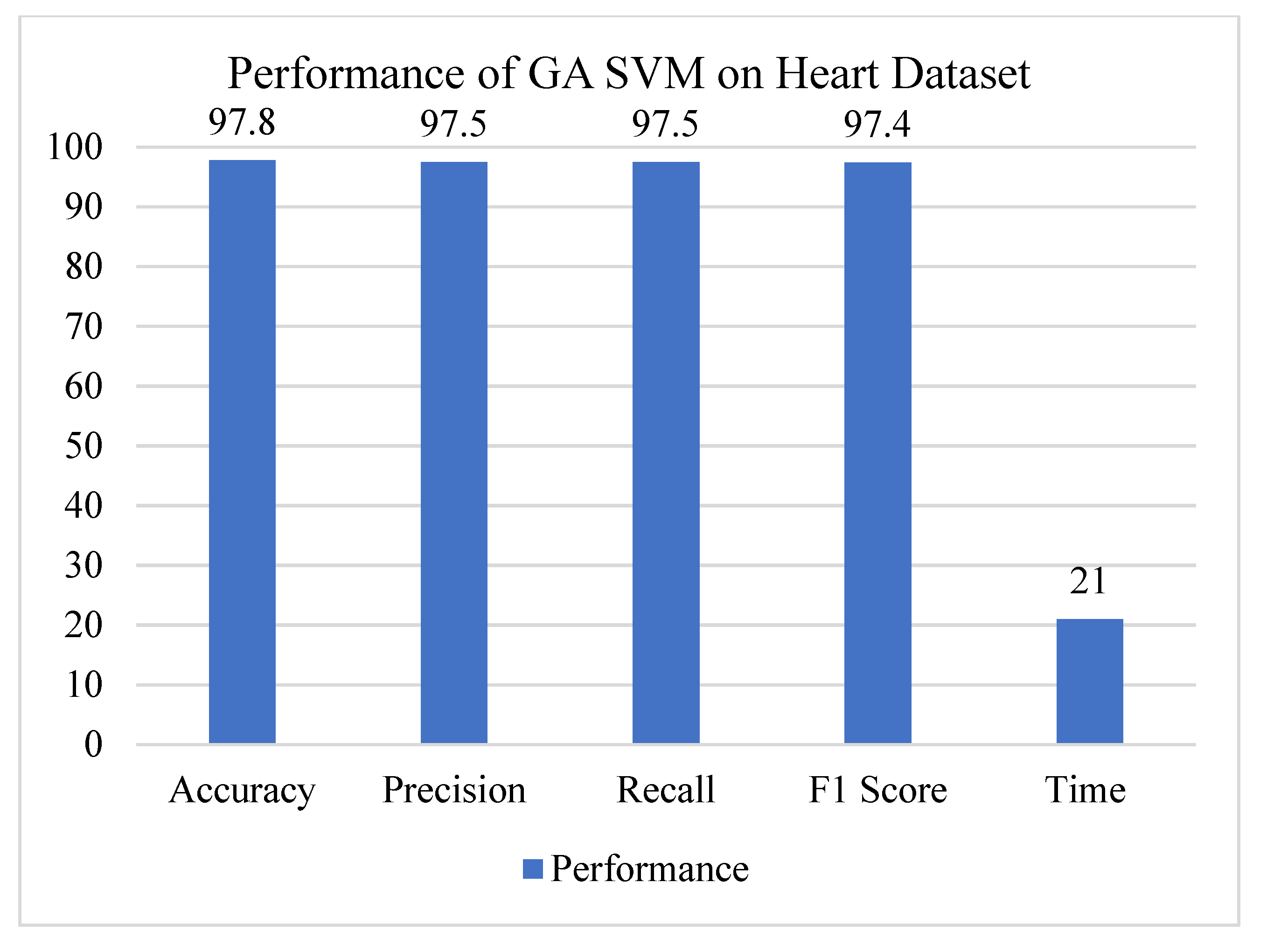
4.3. Performance of GA-SVM

The process of data classification in data mining is made more complicated by the use of genetic algorithms. The process of data classification is broken up into two stages: training and evaluation. During the training phase, a classification model is created, which is subsequently utilised during the classification phase to make input-based predictions about the output. Genes are the fundamental components that distinguish one individual from another. Chromosomes are formed when genes are connected to one another in this way (solution). In a genetic algorithm, the genes of an organism are shown in the form of an alphabetic and numerical string. The usage of binary digits predominates, for the most part (string of 1s and 0s). It is preferable to use a genetic algorithm rather than other strategies that maximise SVM parameters or feature subsets individually because a genetic algorithm has the capacity to optimize both simultaneously. Performance of the GA SVM is shown in Figure 13 and Figure 14.
The selected best GA-SVM parameters are shown in Table 4.

4.4. Performance of WOA-SVM

The Whale Optimization Algorithm (WOA) is a brand-new optimization method that may be applied to a diverse variety of issues. It is named after its namesake, the whale. The three operators in this algorithm that are modelled after the foraging behaviour of humpback whales are called the search for prey operator, the surrounding prey operator, and the bubble-net foraging operator. Iterative execution entails making repeated attempts at a variety of potential solutions until one of those attempts is effective. Since the beginning of the computer age, optimising CAD work processes has been an essential component. In this investigation, we combined WOA with SVM to cut down on the amount of compute required and to improve SVM’s accuracy as shown Figure 15 and Figure 16.
The selected best WOA-SVM parameters are shown in Table 5.

4.5. Performance of PSO-SVM

Computers utilise a method known as particle swarm optimization (PSO), which entails constantly attempting to improve a potential solution in terms of some quality metric, in order to optimize a problem. PSO is an acronym for “particle swarm optimization.” In particular, the PSO algorithm is exceptional when it comes to locating the extremes of functions that are defined on a high-dimensional vector space. In this investigation, we combined PSO with SVM to cut down on the amount of processing time needed and to improve SVM’s accuracy as shown in Figure 17 and Figure 18.
The selected best PSO-SVM parameters are shown in Table 6.

5. Conclusions

The huge magnitude of the endeavor makes fine-tuning the hyperparameters of machine learning algorithms a very difficult operation. We were able to find the most effective method for adjusting the hyperparameters by utilising several algorithmic approaches, such as greedy search and swarm intelligence. Optimization strategies such as random search and grid search have a lot of potential and could be very useful for completing this assignment. The tiny initial population of solutions and expensive objective functions that these searches use can, in some circumstances, lead to a gradual convergence or a prolonged execution time. We used the Support Vector Machine as a model for machine learning, and then we optimized it with the Ant Bee Colony, Genetic Algorithm, Whale Optimization, and Particle Swarm Optimization to evaluate the computation cost of SVM after it had been hypertuned. The computational complexity of these optimization methods was analysed to establish which strategies are the most effective for fine-tuning the hyperparameters. The time complexity of the genetic algorithm was reduced when compared with the time complexity of other algorithms. By making use of the aforementioned four optimization techniques, an investigation like this one might be carried out in the future with the goal of locating the ideal settings for deep learning.

Author Contributions

Conceptualization, E.M.A., Y.A.A. and M.A.-R.; methodology, E.M.A., Y.A.A. and M.A.-R.; software, Y.A.A., A.M. and E.M.A.; validation, E.M.A., A.M. and Y.A.A.; formal analysis, E.M.A., Y.A.A., A.M. and M.A.-R.; investigation, E.M.A., A.M. and Y.A.A.; resources, M.A.-R.; data curation, Y.A.A., E.M.A. and A.M.; writing—original draft preparation, Y.A.A., E.M.A. and A.M.; writing—review and editing, Y.A.A., E.M.A. and M.A.-R.; visualization, Y.A.A. and A.M.; supervision, Y.A.A. and M.A.-R.; project administration, M.A.-R. All authors have read and agreed to the published version of the manuscript.

Funding

The authors extend their appreciation to Deputyship for Research & Innovation, Ministry of Education in Saudi Arabia for funding this research work through the project no. (IFKSURG-2-678).

Data Availability Statement

Publicly available datasets were analyzed in this study. We acquired data on PIMA (Diabetes) from kaggle.com, accessed on 18 November 2022.

Acknowledgments

The authors extend their appreciation to Deputyship for Research & Innovation, Ministry of Education in Saudi Arabia for funding this research work through the project no. (IFKSURG-2-678).

Conflicts of Interest

The authors declare no conflict of interest.

References

  1. Mantovani, R.G.; Rossi, A.L.D.; Vanschoren, J.; Bischl, B.; De Carvalho, A.C.P.L.F. Effectiveness of Random Search in SVM hyperparameter tuning. In Proceedings of the 2015 International Joint Conference on Neural Networks, Killarney, Ireland, 12–17 July 2015. [Google Scholar] [CrossRef]
  2. Dery, L.; Mengistu, R.; Awe, O. Neural Combinatorial Optimization for Solving Jigsaw Puzzles: A Step Towards Unsupervised Pre-Training. 2017. Available online: http://cs231n.stanford.edu/reports/2017/pdfs/110.pdf (accessed on 15 November 2022).
  3. Li, Y.; Zhang, Y.; Cai, Y. A new hyperparameter optimization method for power load forecast based on recurrent neural networks. Algorithms 2021, 14, 163. [Google Scholar] [CrossRef]
  4. Kanimozhi, V.; Jacob, T.P. Artificial intelligence based network intrusion detection with hyperparameter optimization tuning on the realistic cyber dataset CSE-CIC-IDS2018 using cloud computing. In Proceedings of the 2019 International Conference on Communication and Signal Processing (ICCSP), Chennai, India, 4–6 April 2019; pp. 33–36. [Google Scholar] [CrossRef]
  5. Veloso, B.; Gama, J. Self Hyperparameter Tuning for Stream Classification Algorithms. In Proceedings of the Second International Workshop, IoT Streams 2020, and First International Workshop, ITEM 2020, Co-located with ECML/PKDD 2020, Ghent, Belgium, 14–18 September 2020; Communications in Computer and Information Science. Volume 1325, pp. 3–13. [Google Scholar] [CrossRef]
  6. Bergstra, J.; Bardenet, R.; Bengio, Y.; Kégl, B. Algorithms for hyperparameter optimization. In Proceedings of the 25th Annual Conference on Neural Information Processing Systems (NIPS 2011), Granada, Spain, 12–15 December 2011; Advances in Neural Information Processing Systems 24. pp. 1–9. [Google Scholar]
  7. Bergstra, J.; Bengio, Y. Random search for hyperparameter optimization. J. Mach. Learn. Res. 2012, 13, 281–305. [Google Scholar]
  8. Yang, L.; Shami, A. On hyperparameter optimization of machine learning algorithms: Theory and practice. Neurocomputing 2020, 415, 295–316. [Google Scholar] [CrossRef]
  9. Hossain, R.; Timmer, D. Machine Learning Model Optimization with Hyperparameter Tuning Approach. Glob. J. Comput. Sci. Technol. D Neural Artif. Intell. 2021, 21, 7–13. [Google Scholar]
  10. Wang, L.; Feng, M.; Zhou, B.; Xiang, B.; Mahadevan, S. Efficient hyperparameter optimization for NLP applications. In Proceedings of the 2015 Conference on Empirical Methods in Natural Language Processing, Lisbon, Portugal, 17–21 September 2015; pp. 2112–2117. [Google Scholar] [CrossRef]
  11. Escorcia-Gutierrez, J.; Mansour, R.F.; Beleño, K.; Jiménez-Cabas, J.; Pérez, M.; Madera, N.; Velasquez, K. Automated Deep Learning Empowered Breast Cancer Diagnosis Using Biomedical Mammogram Images. Comput. Mater. Contin. 2022, 71, 4221–4235. [Google Scholar] [CrossRef]
  12. Zahedi, L.; Mohammadi, F.G.; Amini, M.H.; Amini, M.H. OptABC: An Optimal Hyperparameter Tuning Approach for Machine Learning Algorithms. In Proceedings of the 2021 20th IEEE International Conference on Machine Learning and Applications (ICMLA), Pasadena, CA, USA, 13–16 December 2021; pp. 1138–1145. [Google Scholar] [CrossRef]
  13. Elgeldawi, E.; Sayed, A.; Galal, A.R.; Zaki, A.M. Hyperparameter tuning for machine learning algorithms used for arabic sentiment analysis. Informatics 2021, 8, 79. [Google Scholar] [CrossRef]
  14. Probst, P.; Boulesteix, A.L.; Bischl, B. Tunability: Importance of hyperparameters of machine learning algorithms. J. Mach. Learn. Res. 2019, 20, 1–32. [Google Scholar]
  15. Andonie, R. Hyperparameter optimization in learning systems. J. Membr. Comput. 2019, 1, 279–291. [Google Scholar] [CrossRef]
  16. Novello, P.; Poëtte, G.; Lugato, D.; Congedo, P. Goal-oriented sensitivity analysis of hyperparameters in deep. J. Sci. Comput. 2023, 94, 45. [Google Scholar] [CrossRef]
  17. Maclaurin, D.; Duvenaud, D.; Adams, R.P. Gradient-based Hyperparameter Optimization through Reversible Learning. In Proceedings of the 32nd International Conference on Machine Learning, Lille, France, 6–11 July 2015; Volume 37. [Google Scholar]
  18. Klein, A.; Falkner, S.; Bartels, S.; Hennig, P.; Hutter, F. Fast Bayesian optimization of machine learning hyperparameters on large datasets. In Proceedings of the 20th International Conference on Artificial Intelligence and Statistics AISTATS 2017, Fort Lauderdale, FL, USA, 20–22 April 2017; Volume 54. [Google Scholar]
  19. Morales-Hernández, A.; Van Nieuwenhuyse, I.; Rojas Gonzalez, S. A survey on multi-objective hyperparameter optimization algorithms for machine learning. Artif. Intell. Rev. 2022. [Google Scholar] [CrossRef]
  20. Pannakkong, W.; Thiwa-Anont, K.; Singthong, K.; Parthanadee, P.; Buddhakulsomsiri, J. Hyperparameter Tuning of Machine Learning Algorithms Using Response Surface Methodology: A Case Study of ANN, SVM, and DBN. Math. Probl. Eng. 2022, 2022, 8513719. [Google Scholar] [CrossRef]
  21. Wu, Q.; Wang, C.; Huang, S. Frugal Optimization for Cost-related Hyperparameters. In Proceedings of the 35th AAAI Conference on Artificial Intelligence, Virtual, 2–9 February 2021; Volume 12A, pp. 10347–10354. [Google Scholar]
  22. ALGorain, F.T.; Clark, J.A. Bayesian Hyperparameter optimisation for Malware Detection. Electronics 2022, 11, 1640. [Google Scholar] [CrossRef]
  23. Liang, Q.; Gongora, A.E.; Ren, Z.; Tiihonen, A.; Liu, Z.; Sun, S.; Deneault, J.R.; Bash, D.; Mekki-Berrada, F.; Khan, S.A.; et al. Benchmarking the performance of Bayesian optimization across multiple experimental materials science domains. Npj Comput. Mater. 2021, 7, 188. [Google Scholar] [CrossRef]
  24. Hazan, E.; Klivans, A.; Yuan, Y. Hyperparameter optimization: A spectral approach. In Proceedings of the 6th International Conference on Learning Representations, ICLR 2018, Vancouver, BC, Canada, 30 April–3 May 2018; Workshop Track Proceedings. pp. 1–18. [Google Scholar]
  25. Van Rijn, J.N.; Hutter, F. Hyperparameter importance across datasets. In Proceedings of the 24th ACM SIGKDD International Conference on Knowledge Discovery & Data Mining, London, UK, 19–23 August 2018; pp. 2367–2376. [Google Scholar] [CrossRef]
  26. Luo, G. A review of automatic selection methods for machine learning algorithms and hyperparameter values. Netw. Model. Anal. Health Inform. Bioinforma. 2016, 5, 18. [Google Scholar] [CrossRef]
  27. Blume, S.; Benedens, T.; Schramm, D. Hyperparameter Optimization Techniques for Designing Software Sensors Based on Artificial Neural Networks. Sensors 2021, 21, 8435. [Google Scholar] [CrossRef] [PubMed]
Figure 1. Proposed flow dataset description.
Processes 11 00349 g001
Figure 2. Features of a dataset with frequency distributions.
Processes 11 00349 g002
Figure 3. Target Outcome in the Heart Dataset.
Processes 11 00349 g003
Figure 4. Data preprocessing.
Processes 11 00349 g004
Figure 5. Feature Correlation Matrix for PIMA Dataset.
Processes 11 00349 g005
Figure 6. Correlation Map for Heart Disease.
Processes 11 00349 g006
Figure 7. ACO-SVM Algorithm.
Processes 11 00349 g007
Figure 8. GA-SVM Algorithm.
Processes 11 00349 g008
Figure 9. WOA-SVM Algorithm.
Processes 11 00349 g009
Figure 10. PSO-SVM Algorithm.
Processes 11 00349 g010
Figure 11. Performance of ACO-SVM on Diabetes.
Processes 11 00349 g011
Figure 12. Performance of ACO-SVM on Heart Disease.
Processes 11 00349 g012
Figure 13. Performance of GA-SVM on Diabetes.
Processes 11 00349 g013
Figure 14. Performance of GA-SVM on Heart Disease.
Processes 11 00349 g014
Figure 15. Performance of WOA-SVM in Diabetes.
Processes 11 00349 g015
Figure 16. Performance of WOA-SVM in Heart Disease.
Processes 11 00349 g016
Figure 17. Performance of PSO-SVM on Diabetes.
Processes 11 00349 g017
Figure 18. Performance of PSO-SVM on Heart Disease.
Processes 11 00349 g018
Table 1. Performance Metrics.
MetricFormula
Cost T n =   n   1
Accuracy Accuracy   =   T   P   +   T   N * T   P   +   T   N   +   F   P   +   F   N .
where
TP   =   True   Positives
TN   =   True   Negatives
FP   =   False   Positives
FN   =   False   Negatives .
Table 2. SVM Parameters.
ParameterDescriptionPossible Values
CThe regularisation parameter. For a given value of C, the regularisation strength decreases. No negatives allowed. A penalty equal to l2 is imposed.float, default = 1.0
DegreePolynomial degree of the kernel function. Totally disregarded by every other kernel out there.int, default = 3
KernelDefines the type of kernel to be used in the algorithm.‘linear’, ‘poly’, ‘rbf’, ‘sigmoid’, ‘precomputed’} or callable, default = ’rbf’
GammaThe ‘rbf,’ ‘poly,’ and ‘sigmoid’ kernel coefficients.{‘scale’, ‘auto’} or float, default = ’scale’
Coef0The kernel function has an independent term. Only in the contexts of poly and sigmoid does it have any bearing.float, default = 0.0
ShrinkingWhether or not to employ the “shrinking heuristic”bool, default = True
ProbabilityAllowing for the calculation of probabilities. A performance hit is noticed when calling fit if this is turned on. The function utilizes 5-fold cross-validation internally, which can take some time, and prediction may not agree with prediction.bool, default = False
ToleranceAcceptable cutoff point for ending.float, default = 1 × 10⁻³
Cache SizeIndicate the amount of space required to dedicate to the kernel cache (in MB).float, default = 200
Class WeightFor SVC, use class weight[i]*C as the value for the class I parameter C. If no other weight is specified, each class is assumed to have a weight of 1. By dividing n samples by (n classes * np.bincount(y)), the “balanced” setting automatically adjusts weights so that they are inversely proportionate to class frequencies in the input data.dict or ‘balanced’, default = None
VerboseSet the output to be very detailed. Be aware that enabling this parameter may cause problems in a multithreaded environment because it relies on a per-process runtime setting in libsvm.bool, default = False
Max IterationsA fixed upper bound on the number of iterations the solver can do, or -1 if there is none.int, default = −1
Decision function shapeWhether to return a decision function of shape (n samples, n classes) similar to that of all other classifiers, or to instead return libsvm’s original one-vs-one (‘ovo’) decision function. To train models, one-on-one (‘ovo’) is always used internally, and an ovr matrix is constructed exclusively from the ovo matrix. However, this parameter is lost in binary classification.{‘ovo’, ‘ovr’}, default = ’ovr’
Random stateControls pseudo random number generation for probability estimation data shuffling. Ignored when probability is False. Pass an int for reproducible output across function calls.bool, default = False
Table 3. Selected best ACO-SVM parameters.
ParameterDescriptionPossible Values
CThe regularisation parameter. For a given value of C, the regularisation strength decreases. No negatives allowed. A penalty equal to l2 is being imposed.default = 1.0
DegreePolynomial degree of the kernel function. Totally disregarded by every other kernel out there.5
KernelDefines the type of kernel to be used in the algorithm.rbf
Table 4. Selected best GA-SVM parameters.
ParameterDescriptionPossible Values
CRegularisation parameter. For a given value of C, the regularisation strength decreases. No negatives allowed. A penalty equal to l2 is being imposed.default = 2.0
DegreePolynomial degree of the kernel function. Totally disregarded by every other kernel out there.4
KernelDefines the type of kernel to be used in the algorithm.linear
Table 5. Selected best WOA-SVM parameters.
ParameterDescriptionPossible Values
CThe regularisation parameter. For a given value of C, the regularisation strength decreases. No negatives allowed. A penalty equal to l2 is being imposed.default = 2.0
KernelDefines the type of kernel to be used in the algorithm.polynomial
Table 6. Selected best PSO-SVM parameters.
ParameterDescriptionPossible Values
CThe regularisation parameter. For a given value of C, the regularisation strength decreases. No negatives allowed. A penalty equal to l2 is being imposed.default = 2.0
KernelDefines the type of kernel to be used in the algorithm.polynomial
Class WeightFor SVC, use class weight[i]*C as the value for the class I parameter C. If no other weight is specified, each class is assumed to have a weight of 1. By dividing n samples by (n classes * np.bincount(y)), the “balanced” setting automatically adjusts weights so that they are inversely proportionate to class frequencies in the input data.True
VerboseSet the output to be very detailed. Be aware that enabling this parameter may cause problems in a multithreaded environment because it relies on a per-process runtime setting in libsvm.False
Disclaimer/Publisher’s Note: The statements, opinions and data contained in all publications are solely those of the individual author(s) and contributor(s) and not of MDPI and/or the editor(s). MDPI and/or the editor(s) disclaim responsibility for any injury to people or property resulting from any ideas, methods, instructions or products referred to in the content.

