An Integrated Method of Bayesian Optimization and D-Optimal Design for Chemical Experiment Optimization

Abstract

The smart chemical laboratory has recently emerged as a promising trend for future chemical research, where experiment optimization is of vital importance. The traditional Bayesian optimization (BO) algorithm focuses on exploring the dependent variable space while overlooking the independent variable space. Consequently, the BO algorithm suffers from becoming stuck at local optima, which severely deteriorates the optimization performance, especially with bad-quality initial points. Herein, we propose a novel stochastic framework of Bayesian optimization with D-optimal design (BODO) by integrating BO with D-optimal design. BODO can balance the exploitation in the dependent variable space and the exploration in the independent variable space. We highlight the excellent performance of BODO even with poor initial points on the benchmark alpine2 function. Meanwhile, BODO demonstrates a better average objective function value than BO on the benchmark Summit SnAr chemical process, showing its advantage in chemical experiment optimization and potential application in future chemical experiments.

1. Introduction

The application of advanced machines and technologies is significantly driving chemical research evolving toward digitalization and automation, along with huge convenience and high efficiency in the favor of chemists and chemical engineers [1]. With the foundation of automation technology, the smart chemical laboratory is devoted to freeing researchers from tedious and repetitive experiments, as well as greatly improving scientific research efficiency, through a rational experiment optimization process [2,3]. Traditional experiment design heavily relies on the researcher’s knowledge or experience to optimize the experiment output. On the contrary, a smart laboratory is supposed to leverage the optimization algorithm for efficient experiment space exploration [4]. Optimization algorithm-based iterative experimentation has undoubtedly become a prevailing trend for the future laboratory, and many laboratories have joined this trend to reform their experiments toward high-performance material synthesis [5], optimal procedure design [6], process parameter optimization [7], and so on [8,9]. For most chemical experiments to be researched, on one hand, a first-principle model is usually lacked as a rigorous description of the chemical process [10,11,12]; on the other hand, it is often the case that experiment data is insufficient to establish a solid data-driven model, especially for those experiments that are time- or resource-consuming (or both) [13]. Therefore, it is important to develop an efficient optimization algorithm that iteratively recommends experiment points to search for optimal experiment conditions. In this sense, the experiment optimization algorithm plays a central role in experiment space exploration and drives scientific research in the future smart chemical laboratory [14].

In recent years, increasing research fields have started to focus on the use of experiment algorithms to assist scientific research [15,16]. Some scholars attempted to describe the whole experiment space with machine learning methods and then search for optimal solutions using as-established models [17,18]. Zhou et al. proposed a machine learning framework named MiYa to optimize heterologous metabolic pathways in saccharomyces cerevisiae, using the voting results of computational recommendations of multiple neural network models [19]. Using artificial neural networks, Burre et al. approximated thermodynamic models for reductive dimethoxymethane synthesis and achieved a high energy efficiency of 91.9%, with their developed deterministic global optimization solver MAiNGO [20]. Machine learning delivers a relatively higher fitting accuracy when compared to traditional regression models [21], such as vanilla polynomial regression [22], ridge regression [23], and partial least squares regression [24]. However, due to the data amount requirement of machine learning, collected data samples are generally not enough to describe the overall experiment space for emerging chemical processes, resulting in overfitting, poor generalization, and unreliable prediction, which significantly hinders the application of machine learning models [25,26].

In the scenario of data scarcity, the experiment optimization algorithm can be resorted to as an alternative solution to optimize the experiment conditions, and has received a lot of attention in recent years [27]. Lapkin’s group applied experiment optimization algorithms to green chemical processes, and these algorithms showed a significant potential in promoting the sustainability of versatile chemical products in their entire life cycles [28,29]. In addition, they developed open-source benchmark processes and fundamental optimization strategies as a set of tools toward chemical process optimization, which is available at https://github.com/sustainable-processes/summit (accessed on 20 August 2019) [30]. Among various optimization algorithms, Bayesian optimization (BO) is one of the most-used algorithms, which operates in the dependent variable space and exhibits two major advantages: one is that BO employs the GP regression as its inner surrogate model, of which the results depict not only the prediction value but also the confidence degree over the experiment space; the other one is that BO is well fitted with the iterative experiment process, during which the surrogate model can evolve to be more and more reliable with new experimental data gradually added into the dataset [31]. BO has been used in many chemical experiments with high experiment costs. Sun et al. combined BO with a first-principle model to conveniently identify the most stable alloyed organic–inorganic perovskites [32]. Xue et al. utilized BO to accelerate the search of BaTiO₃-based piezoelectric materials with vertical morphological phase boundaries [33]. Apart from single-task optimization, BO is also helpful for chemical process with multiple targets, which usually include space–time yield, by-product formation, and product selectivity. For example, Jorayev et al. simultaneously optimized yield and conversion of the chemical route from a mixture of waste terpenes to p-cymene using multi-objective BO [34]. Despite the fact that BO performs excellently in experiment optimization with small datasets, BO is defined to search in the dependent variable space using surrogate model prediction and overlooks searching in the independent variable space from the perspective of experiment design [35]. Moreover, BO is strongly dependent on the initial data points and tends to fall into local optima when starts with points of bad quality [36].

To address this problem, we introduce the design of experiments (DoE) into BO to complement its weakness in terms of initial point reliance and rational iterative experiment recommendation [37]. DoE aims to select the most informative point locations in the experiment space to facilitate mathematical statistics and analysis after experiments [38]. Optimal design is a typical class of DoE utilized, usually as an initial point selection aid, to accommodate multiple types of factors in the independent variable space with respect to a specific statistical criterion [39]. Herein, we propose Bayesian optimization with D-optimal design (BODO) as an integrated stochastic optimization framework to improve the optimization efficiency of chemical experiments. The D-optimal design criterion is a representative DoE criterion that aims at maximizing the differential Shannon information of recommended points in the experiment space [40,41]. In each experimental iteration of BODO, the recommendation point is stochastically derived from the BO branch or the D-optimal design branch. In the D-optimal design branch, candidate recommendation points can be given by batch Bayesian optimization with local penalization (BBOLP) [42] or random selection. The final recommendation is the candidate point with the maximal D-optimal design criterion value. The BO branch is an exploitation process based on the surrogate model prediction in the dependent variable space; The D-optimal design branch is an exploration in the independent variable space for the most informative experiment point. With this stochastic two-branch design, BODO achieves a tradeoff between exploitation and exploration, and thus is expected to relieve the dependency on initial point selection and contribute to optimal experiment condition search.

2. Preliminaries

2.1. Bayesian Optimization

Problem definition: Assume that $f$ is a black-box function, of which the mathematical form is unknown and it is time-consuming to generate evaluations for this function. Let $f:\mathcal{X}\to ℛ$ be a function defined on a subset $\mathcal{X}\subseteq {ℛ}^D$. Here $D$ indicates the dimension of the subset ${ℛ}^D$. The goal is to solve the optimization problem expressed as Equation (1):

$$x^{*}=\underset{x\in \mathcal{X}}{\mathrm{argmax} }f\left(x\right)$$

(1)

BO is a sequential design optimization algorithm for the black-box function that does not assume any functional form. There are two main components in the BO framework: the surrogate model and the acquisition function [43]. In each iteration, a surrogate model (e.g., Gaussian process regression) is established with experiment data already obtained, and this surrogate model is capable of giving out both the prediction value and the standard deviation of the dependent variable. Then, a predefined acquisition function measures the extent to which each point is worth a practical experiment through concurrent consideration of maximizing the prediction value and the uncertainty. Finally, the experiment point with the maximal value of the acquisition function is solved as the next experiment point. The pseudocode of BO is presented in Algorithm 1.

Algorithm 1. The pseudocode of BO.

Input: Dataset ${\mathcal{D}}_0={\left\{(x_i, y_i)\right\}}_{i=1}^n$

for $t=1$ to $T$ do    Fit Gaussian process model and acquisition function ${\alpha }_t\left(x\right)$ on ${\mathcal{D}}_{t-1}$    Solve $x_t\leftarrow \underset{x\in \mathcal{X}}{\mathrm{argmax}} {\alpha }_t\left(x\right)$   Evaluate $y_t\leftarrow f\left(x_t\right)$   Take ${\mathcal{D}}_t={\mathcal{D}}_{t-1}{\displaystyle \cup }\left\{(x_{\mathrm{t}}, y_t)\right\}$  end for

Output:${\mathcal{D}}_T$

Gaussian process: GP is the most common surrogate model used in BO [44]. GP associates a normally distributed random variable at each point of the input dataset. In this work, GP is given as $GP\left(\mu \left(x\right),k\left(x,x^{\prime }\right)\right)$, where $\mu \left(x\right)$ is the mean function (Equation (2)) and $k\left(x,x^{\prime }\right)$ is the kernel function representing the covariance of any two observations. The variance ${\sigma }^2\left(x\right)$ is given as Equation (3). $K_{i,j}$ indicates the value at row $i$ and column $j$ of $K$, which equals $k\left(x_i,x_j\right)$ (Equation (4)). $k_{*}$ is defined as the variance between a candidate data point ($x$) and all current observations (${\left\{x_i\right\}}_{i=1}^n$) (Equation (5)).

$$\mu \left(x\right)=k_{*}{K}^{-1}y$$

(2)

$${\sigma }^2\left(x\right)=k\left(x,x\right)-k_{*}{K}^{-1}{k}_{*}^T$$

(3)

$$K_{i,j}=k\left(x_i,x_j\right)$$

(4)

$$k_{*}=\left(k\left(x,x_1\right),\dots ,k\left(x,x_n\right)\right)$$

(5)

Acquisition function: The acquisition function $\alpha \left(x\right)$ is used to map the estimated mean and standard deviation at a candidate point to its value for a practical experiment. Routinely, the upper confidence bound (UCB) is used as the acquisition function, which is calculated using Equation (6). $\kappa$ is a parameter to balance the weights between the predicted mean value and standard deviation of the GP model.

$$\alpha \left(x\right)=\mu \left(x\right)+\kappa \sigma \left(x\right)$$

(6)

2.2. Local Penalization

BBOLP is a variant of BO, which recommends a batch of points in each iteration and of which the acquisition function is modified with local penalization (LP). BBOLP is a heuristic approach by iteratively penalizing the acquisition function value of the recommended point to find the next experiment point [42]. The BBOLP algorithm is given in Algorithm 2.

Algorithm 2. The pseudocode of BBOLP.

Input: Dataset ${\mathcal{D}}_0={\left\{(x_i, y_i)\right\}}_{i=1}^n$, Batch size $n_b$

for $t=1$ to $T$ do    Fit Gaussian process model and acquisition function ${\alpha }_t\left(x\right)$ on ${\mathcal{D}}_{t-1}$    Take ${\tilde{\alpha }}_{t,0}\leftarrow g\left({\alpha }_t\left(x\right)\right)$ and $\widehat{L}\leftarrow \underset{x\in \mathcal{X}}{\max }\Vert {\mu }_{\nabla }\left(x\right)\Vert$    for $j=1$ to $n_b$ do       Maximization step: $x_{t,j}\leftarrow \underset{x\in \mathcal{X}}{\mathrm{argmax}} {\tilde{\alpha }}_{t,j-1}\left(x\right)$       Penalization step: ${\tilde{\alpha }}_{t,j}\left(x\right)\leftarrow {\tilde{\alpha }}_{t,0}\left(x\right){\displaystyle \prod }_{j=1}^k\phi \left(x;x_{t,j},\widehat{L}\right)$    end for    Take ${ℬ}_t\leftarrow \left\{x_{t,1},\dots ,x_{t,n_b}\right\}$    Parallel evaluate $y_{t,1},\dots , y_{t,n_b}$ in ${ℬ}_t$    Take ${\mathcal{D}}_t={\mathcal{D}}_{t-1}{\displaystyle \cup }{\left\{(x_{t,j}, y_{t,j})\right\}}_{j=1}^{n_b}$  end for

Output:${\mathcal{D}}_T$

The acquisition function with LP is composed of two steps: the maximization step is to find out the point that achieves the maximum value of the current acquisition function; once the maximization step is completed, the penalization step multiplies the acquisition function with an LP operator $\phi \left(x;x_j, \widehat{L}\right)$ to avoid the next sampling point being too close to the current one. $\phi \left(x;x_j, \widehat{L}\right)$ measures the distance between the current point with any other sampled point in the search space, and output with a value between 0 and 1 as the penalization factor. $\phi \left(x;x_j, \widehat{L}\right)$ can be written as:

$$\phi \left(x;x_j,\widehat{L}\right)=\frac{1}{2}erfc\left(-z\right)=\frac{2}{\sqrt{\pi }}{{\displaystyle \int }}_{-z}^{\infty }{e}^{-{\eta }^2}d\eta$$

(7)

$$z=\frac{1}{\sqrt{2{\sigma }_n^2\left(x_j\right)}}\left(\widehat{L}\Vert x_j-x\Vert -\underset{x\in \mathcal{X}}{\max } f\left(x\right)+{\mu }_n\left(x_j\right)\right)$$

(8)

where $erfc$ is a complementary error function that outputs a value ranging from 0 to 2 and $\widehat{L}$ represents the Lipschitz constant. Since the penalty is applied to the acquisition function by multiplying, when the value of the acquisition function is negative, it would mistakenly act as positive feedback which increases the value of the acquisition function in this region. Therefore, a regularization function is utilized to adjust the acquisition function output and ensure that any output value of the acquisition function is positive. The used regularization function can be written as Equation (10).

$$g\left(z\right)=\{\begin{array}{ll}z,& z\ge 0\\ ln\left(e^z+1\right),& z<0\end{array}$$

(9)

2.3. D-Optimal Design

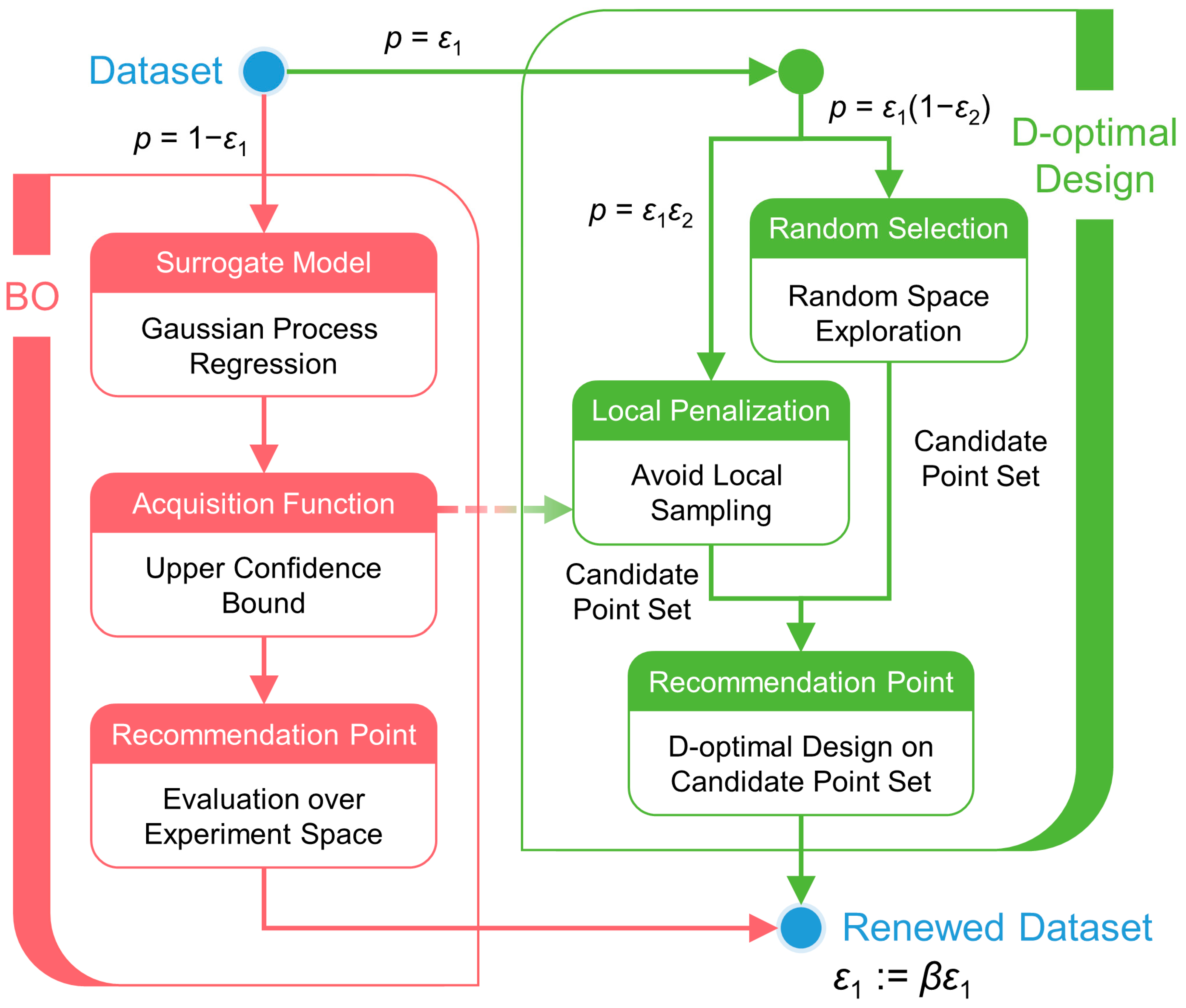
Optimal design is a class of DoE methods that are optimal with respect to some well-defined statistical criterion. In the DoE for estimating statistical models, the optimal design allows parameters to be estimated with minimum variance and without bias. The core idea of the optimal design criterion is to make the sampled points in the independent variable space as dispersed as possible. A non-optimal design requires more experimental runs to estimate the parameters with the same precision as an optimal design.

The D-optimal design criterion is an optimal design criterion devoted to maximizing the differential Shannon information content of parameter estimates. Assume the existing dataset is ${\{(x_i,y_i)\}}_{i=1}^n$ and the next point candidate set is ${\left\{{\overline{x}}_j\right\}}_{j=1}^m$. For each point in the candidate set, the D-optimality is calculated as the determinant value of the information matrix. The information matrix can be expressed as $D_{\mathrm{j}}=\det (A_{\mathrm{j}}{A}_{\mathrm{j}}^{\mathrm{T}})$, where $A_{\mathrm{j}}$ considers first-order and second-order terms, and is set as $\left[1,x_1,x_2,\dots ,x_n,{\overline{x}}_j,x_1^2,x_2^2,\dots ,x_n^2,{\overline{x}}_j^2\right]$. The candidate point with the maximal D-optimality value is considered to be able to minimize the prediction variance the most. Therefore, this point is selected for the next experiment iteration according to this D-optimal design criterion.

3. Methodology

In this work, we propose BODO as a novel experiment optimization method by integrating BO with D-optimal design in a stochastic framework. Although BO has already demonstrated good performance in many chemical experiments with limited available data, it only operates in the dependent variable space and focuses on fast optimization at the expense of global search capability. This would lead to a tendency for BO to fall into local optimum solutions in some complex systems, especially when applied with bad-quality initial points. The main idea of our proposed BODO is to introduce a bypass branch that operates in the independent variable space into BO. The introduced bypass branch is based on the D-optimal design criterion to balance local and global search performance in experiment iteration. The BODO framework for experiment optimization is displayed in Figure 1.

In the BODO framework, ${\epsilon }_1$, ${\epsilon }_2$, and $\beta$ are three hyperparameters that balance the probabilities of all branches for experiment point recommendation. In each iteration, the probability that the final recommended point is generated by the BO branch (red part in Figure 1) is $1-{\epsilon }_1$. The architecture of BO is the same as introduced in Section 2.1. The surrogate model and the acquisition function are GP regression and UCB, respectively. BODO is designed to search the independent variable space through the introduced D-optimal design branch (green part in Figure 1) with a probability of ${\epsilon }_1$. In the D-optimal design branch, a candidate point set can be created by either BBOLP or random selection. Then, the points in the candidate set are evaluated by the D-optimal design criterion to select the final recommended point for the next experiment. The probability distribution between BBOLP and random selection is adjusted by the hyperparameter ${\epsilon }_2$. The BBOLP candidate point set is proposed in the light of already observed points and the randomly selected candidate point set can explore the experiment space to a greater extent. The pseudocode for BODO is given in Algorithm 3. A hyperparameter $\beta \in \left(0,1\right)$ is further introduced as a decline factor of ${\epsilon }_1$ to dynamically tune the probability of exploration after each iteration. At the beginning stage, it is rational to assign BODO with a greater probability of exploring the experiment space. As the iteration progresses, BODO should gradually be more inclined to exploitation than exploration. This is realized by multiplying ${\epsilon }_1$ with the defined decline factor $\beta$ after each iteration.

Algorithm 3. The pseudocode of BODO.

Input: Dataset ${\mathcal{D}}_0={\left\{(x_i, y_i)\right\}}_{i=1}^n$, ${\epsilon }_1$, ${\epsilon }_2$, $\beta$, Candidate point set size $n_c$

for $t=1$ to $T$ do    Fit Gaussian process model and acquisition function ${\alpha }_t\left(x\right)$ on ${\mathcal{D}}_{t-1}$    Take $m_1, m_2=random\left(0, 1\right)$    if $m_1>{\epsilon }_1$ then      Solve $x_t\leftarrow \underset{x\in \mathcal{X}}{\mathrm{argmax}} {\alpha }_t\left(x\right)$    else    if $m_2>{\epsilon }_2$ then        $X_t\leftarrow$ random select $n_c$ samples from $\mathcal{X}$      else           ${\tilde{\alpha }}_{t,0}\leftarrow g\left({\alpha }_t\left(x\right)\right)$           $\widehat{L}\leftarrow \underset{x\in \mathcal{X}}{\max } \Vert {\mu }_{\nabla }\left(x\right)\Vert$        for $j=1$ to $n_c$ do          Maximization step: $x_{t,j}\leftarrow \underset{x\in \mathcal{X}}{\mathrm{argmax}} {\tilde{\alpha }}_{t,j-1}\left(x\right)$          Penalization step: ${\tilde{\alpha }}_{t,j}\left(x\right)\leftarrow {\tilde{\alpha }}_{t,0}\left(x\right){\displaystyle \prod }_{j=1}^k\phi \left(x;x_{t,j},\widehat{L}\right)$        end for           $X_t\leftarrow \left\{x_{t,1}, \dots , x_{t,n_c}\right\}$    end if    for $x_{t,i}\in X_t$ do        $A_{t,i}=\left[1,x_1,x_2,\dots ,x_n,x_{t,i}, x_1^2,x_2^2,\dots ,x_n^2,x_{t,i}^2\right]$        $D_{t,i}=\det \left(A_{t,i}{A}_{t,i}^T\right)$      end for          $x_t\leftarrow \underset{x_{t,i}\in X_t}{\mathrm{argmax}} D_{t,i}$    end if    evaluate $y_t\leftarrow f\left(x_t\right), {\epsilon }_1\leftarrow \beta {\epsilon }_1$    Take ${\mathcal{D}}_t={\mathcal{D}}_{t-1}{\displaystyle \cup }\left\{(x_t, y_t)\right\}$  end for

Output:${\mathcal{D}}_T$

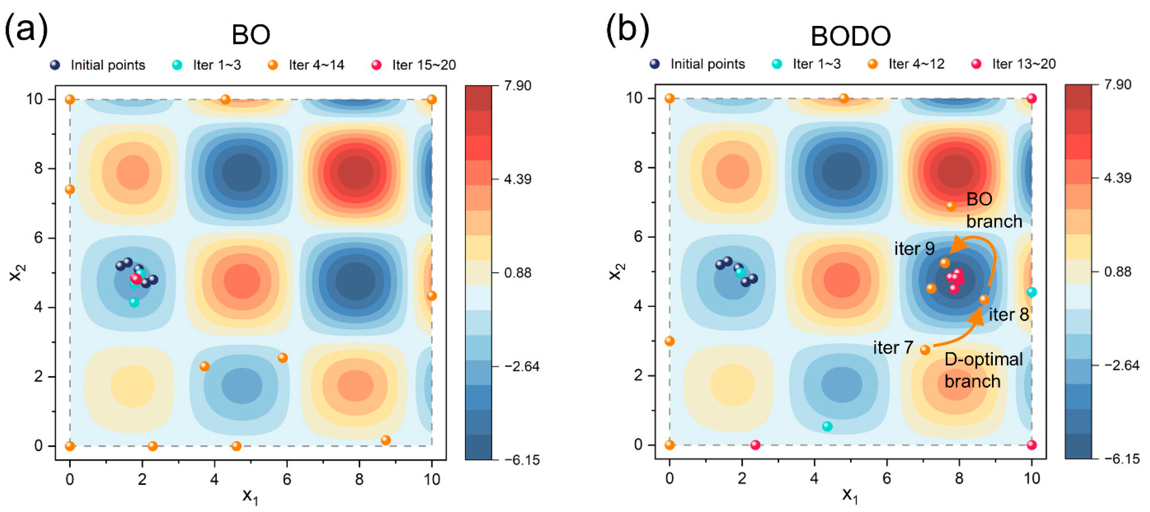
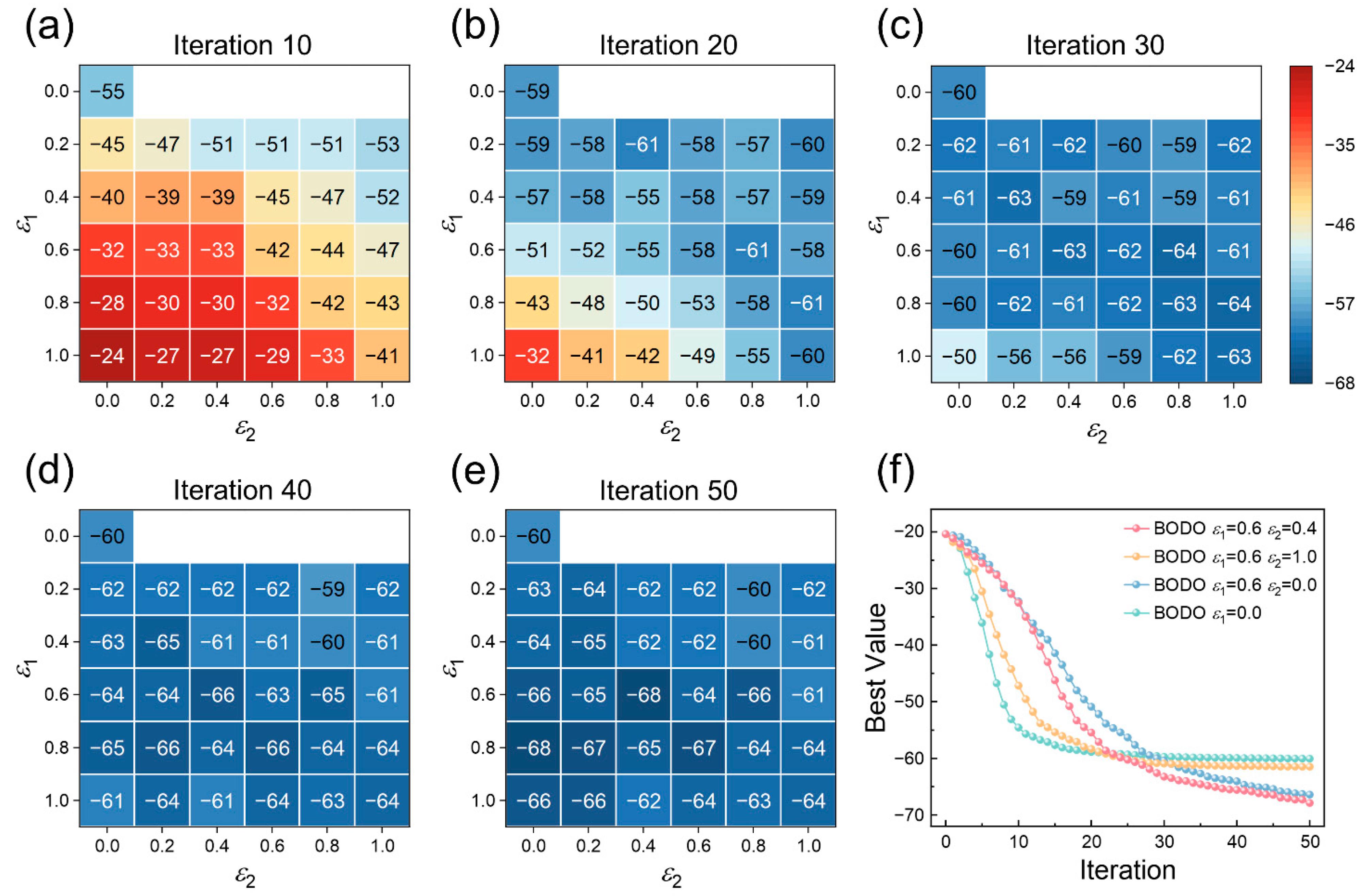
4. Results and Discussion

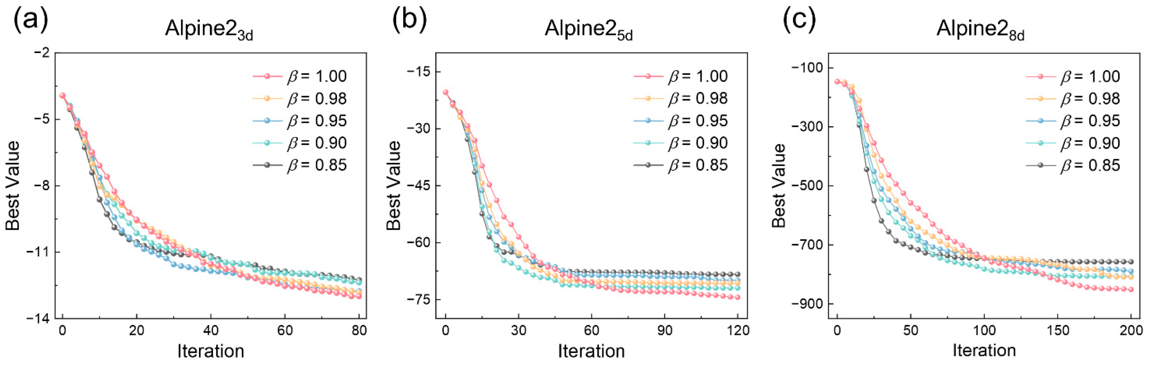
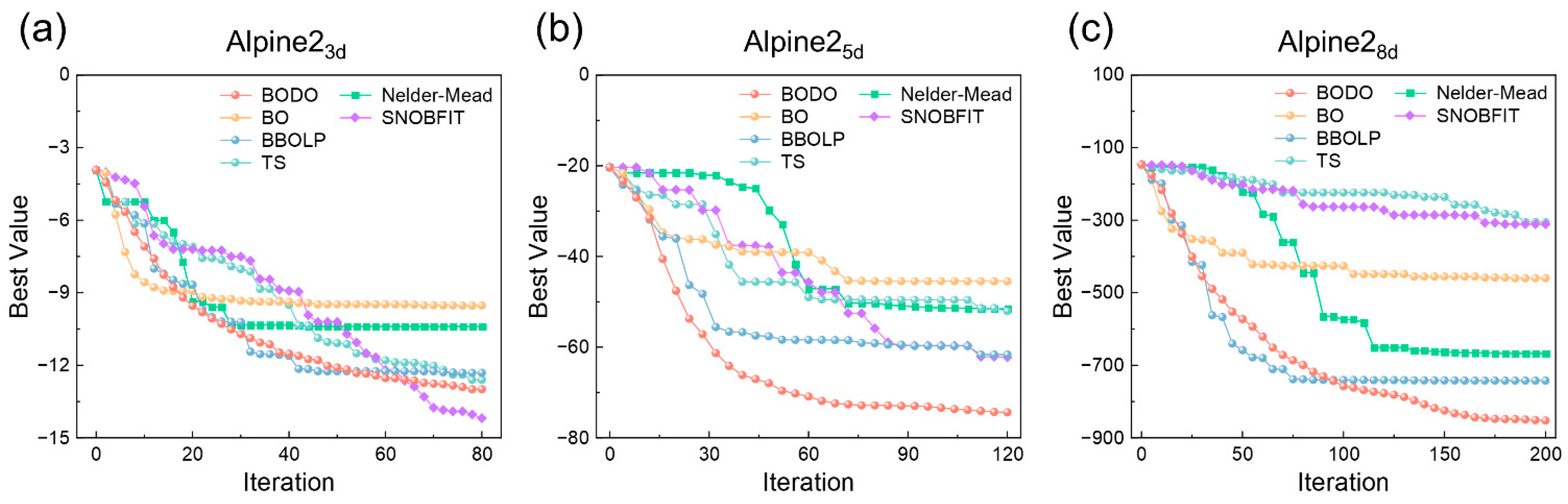
4.1. Benchmark alpine2 Function

In this work, we use the benchmark alpine2 test functions with different dimensions to test the performance of BODO and compare it with other approaches such as BO. The alpine2 function can be expressed as Equation (10), of which the definition domain of any $x_i$ is [0,10]. The alpine2 function contains multiple local minima in the domain range and is thus suitable for the validation of the experiment optimization algorithm. The theoretical minimal value for the alpine2 function is $-2.18\times {2.81}^{n-1}$, where $n$ is the input dimension size. The minimization optimization problem can be transformed into a maximization one by adding a minus sign.

$$f_{\mathrm{alpine}2}\left(x\right)={\displaystyle \prod }_{i=1}^n\sqrt{x_i}\sin \left(x_i\right)$$

(10)

For the test settings, the number of initial points $n_0$ was set to $3\times D$. Matern52 was used as the kernel of GP regression in BODO and BO. Matern52 can be expressed as Equation (11). $\Gamma$ and $K_{\nu }$ respectively represent the gamma function and the Bessel function of the second kind. $d\left(x_i,x_j\right)$ indicates the distance between $x_i$ and $x_j$. The parameter $\nu$ of Matern52 was fixed to $5/2$ and the covariance $l$ was fixed to $1$. UCB was used as the acquisition function and the parameter $\kappa$ of Equation (6) was set to 2.

$$k\left(x_i,x_j\right)=\frac{1}{\Gamma \left(\nu \right)2^{\nu -1}}{\left(\frac{\sqrt{2\nu }}{l}d\left(x_i,x_j\right)\right)}^{\nu }{K}_{\nu }\left(\frac{\sqrt{2\nu }}{l}d\left(x_i,x_j\right)\right)$$

(11)

Figure 2 is the visualization results of BO and BODO on the alpine2_2d test function with initial points of bad quality. The preset initial points are all near a local optimum. The iteratively recommended point locations are marked on the contour image of alpine2_2d, with different colors indicating different iteration segments.

Figure 2a intuitively shows the optimization process of BO, which is a deterministic algorithm based on UCB. The first 3 recommended points by BO are located near the initial local optimum since the surrogate model prediction is relatively more optimal in this region. Most recommended points of BO from iteration 4 to iteration 14 are located at the boundary, which is the result of a larger variance of the GP model. In the final six iterations, BO converges back to the initial local optimum. In comparison, BODO adopts a D-optimal design branch allowing for the method to sample over the experiment space from the information perspective (Figure 2b). The strategy of BO heavily relies on its inner surrogate model, which usually requires representative initial points for generalized prediction. In this alpine2_2d case, BODO is able to discover the global optimum region with poor initial points and further exploits near the optimum. This optimum region is discovered by the point recommended by the D-optimal branch at iteration 8 and the following point recommended by BO at iteration 9. This small example visually illustrates the improvement of BODO in initial point dependence relief and local optimum avoidance.

The effects of different ${\epsilon }_1,{\epsilon }_2$ settings are investigated also in this work (Figure 3), with a value of $\beta$ fixed at 0.95. Each result is derived as the average of 10 runs at 10 different random initial point sets (100 runs in total), and in each run BODO is iterated for 50 rounds.

If ${\epsilon }_1$ is set to 0.0, the D-optimal design branch in BODO is prohibited and BODO will degrade into BO. It is noteworthy that a ${\epsilon }_1$ value of 1.0 does not mean that BODO only carries out the D-optimal design branch, because ${\epsilon }_1$ is supposed to be multiplied with $\beta$ and decline after each iteration. Figure 3a–e plots the heatmaps of the best values of BODO with different hyperparameter settings at different iterations. It can be observed that BODOs with relatively smaller ${\epsilon }_1$ values can find a better solution than those with larger ones at the beginning, but can hardly make any further progress after 30 iterations. The BO method falls into a local optimum after approximately 30 iterations, and its average best value remains −60 in subsequent iterations. In comparison, BODOs with relatively larger ${\epsilon }_1$ can still find better solutions after 40 iterations, and the best BODO (${\epsilon }_1=0.6$, ${\epsilon }_2=0.4$) achieves an average best value of −68, much smaller than that of BO. It can be demonstrated that the introduced D-optimal design branch is helpful to jump out of local optima and contributes to the optimization process. Additionally, Figure 3f manifests that BODO with both LP and random selection outperforms BODO with either one of them and degraded BODO, showing the synergistic effect of LP and random selection in the D-optimal design branch.

To explore how BO and BODO (${\epsilon }_1=0.6,{\epsilon }_2=0.4$) perform with different initial point sets in detail, the results of different initial point sets are separately plotted in Figure 4a, including the result best value of BO and the average, minimal, and maximal best value of BODO. The number of points in the initial point set was 9 for BO and BODO, which are separately applied to 10 different initial point sets. On almost all initial point sets, BODO has a better average search result than BO. For initial point sets 2, 3, 4, and 8, the performance of BODO is equivalent to that of BO. For the other six initial point sets, BODO outperforms BO by an obvious improvement on the final best value. Moreover, for initial point sets except 6 and 9, even the worst BODO results are better or similar to those of BO. Comparing BO with BODO, it can be found BO would be stuck in local optima with initial point sets 1, 5, 7, and 10, while BODO can possibly jump out of local optima and find better solutions. Figure 4b shows the iteration process of BO and the 10 runs of BODO with the initial point 7. After about 10 iterations, the deterministic BO algorithm falls into a local optimum. Although the BODO average best value decreases slower than BO at the beginning stage, it can continuously be optimized. After 50 iterations, even the worst run of BODO reaches the same best value as BO and the best run of BODO finds a solution with an objective function value of −135.68, which should be attributed to the D-optimal design branch. Therefore, it can be concluded that the introduction of the D-optimal design can assist the experiment optimization algorithm to leverage the exploration in the independent variable space and promote the experiment optimization performance.

In BODO, $\beta$ is a key parameter to determine the decline speed of the probability of the D-optimal design branch. To figure out the effect of $\beta$ on systems with different dimensions, alpine2_3d, alpine2_5d, and alpine2_8d were adopted for investigation. ${\epsilon }_1$ was fixed to 0.6 and ${\epsilon }_2$ was fixed to 0.4. The iteration rounds of alpine2_3d, alpine2_5d, and alpine2_8d were set to 80, 120, and 200, respectively. For each alpine2 test function, BODOs with different $\beta$ values were run with 10 different random initial point sets for 10 times. The BODO average optimization results are displayed in Figure 5.

For all alpine2 test functions, the best value decreases faster in the early stage when $\beta$ is set smaller. This is because a smaller $\beta$ value means a relatively larger probability in the BO branch for exploitation. However, after a certain number of iterations, a larger $\beta$ value can lead to a better best value for its inclination toward exploration through the D-optimal branch. With regard to the final best value, the best $\beta$ setting is 1.00 for all alpine2 test functions because the exploration probability does not decrease with the experiment iteration. These results show that more attention should be paid to exploration for a better final best value if the experiment can be iterated with enough rounds. Meanwhile, a smaller $\beta$ value is recommended for fast experiment optimization when the number of experiment iterations is strictly limited.

In Figure 6a–c, BODO is compared with some other optimization algorithms on the alpine2_3d, alpine2_5d, and alpine2_8d test functions, respectively. The comparing algorithms include BO, BBOLP, Thompson sampling (TS), Nelder–Mead, and stable noisy optimization by branch and fit (SNOBFIT). TS is also a GP-based algorithm for experiment optimization which trains a GP model for the objective and then applies spectral sampling to the trained GP for experiment recommendation [45]. Nelder–Mead is a simplex optimization method which includes adaptions of point reflection, dimension reduction, and dimension recovery [46]. SNOBFIT adopts a branching algorithm that recursively divides the search space into smaller regions from which evaluation points are chosen for experiments [47]. In this way, SNOBFIT is capable of generating points in unexplored regions and presents a global search ability. BODO outperforms all other GP-based methods on all alpine2 test functions, especially on alpine2 test functions with relatively larger dimension sizes. BO suffers from the lack of exploration ability in the independent variable space. TS also focuses only on the fitted GP model and is inferior in terms of exploration. BBOLP adopts a penalization strategy to avoid the recommended points located in a small region, but still lacks a guidance of point distribution in the independent variable space. As for other comparing methods, Nelder–Mead is a simplex method and therefore its optimization efficiency is unavoidably lower. As a global optimization method, SNOBFIT suggests a better final optimization result than BODO in alpine2_3d. However, since SNOBFIT divides the entire experiment space into subregions and can only recommend points in unexplored subregions that are located near explored ones, its convergence speed is consequently slow, which can be revealed by results on alpine2_5d, alpine2_8d, and the first 40 iterations of alpine2_3d. These comparison results demonstrate the effectiveness of BODO in balancing exploitation and exploration, as well as an outstanding feasibility in optimization problems with different input dimension sizes.

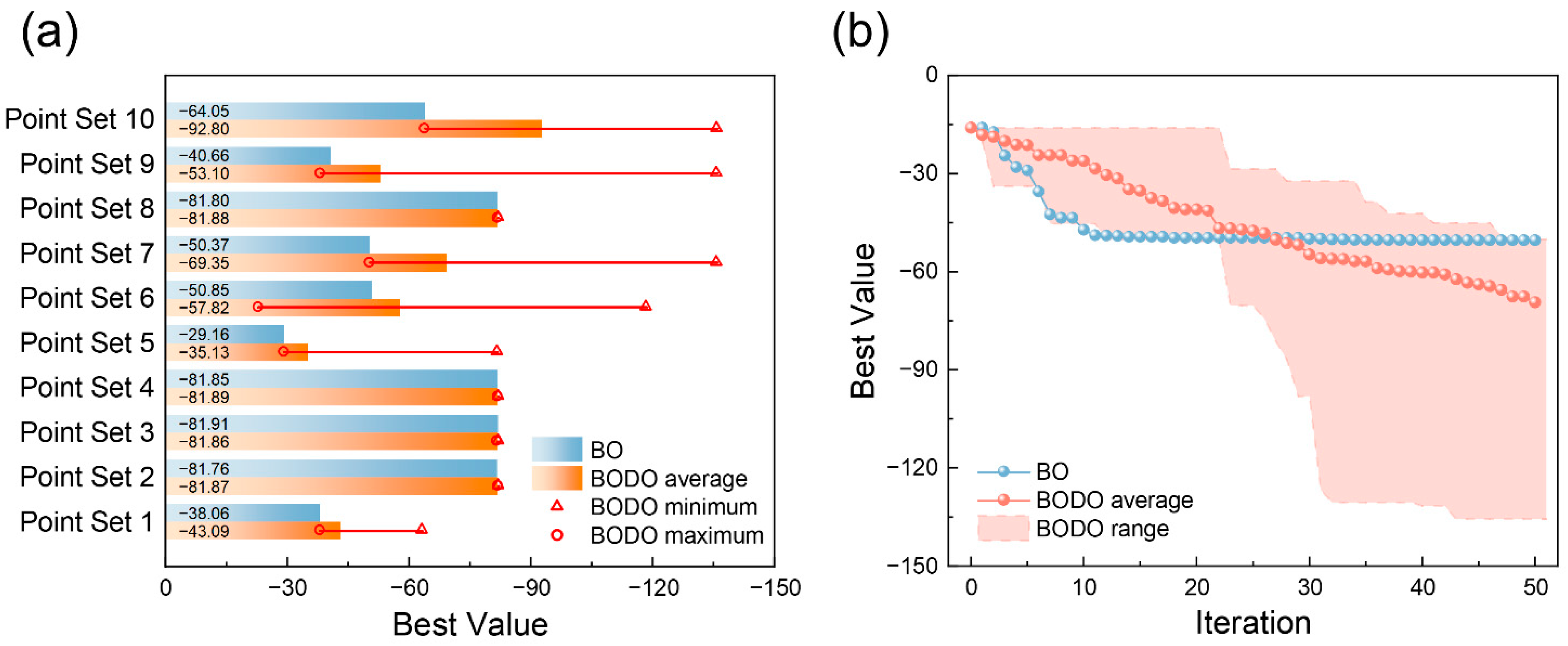
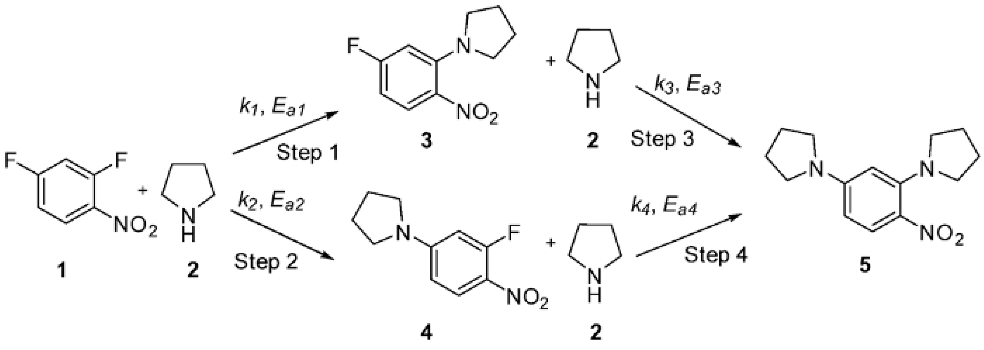
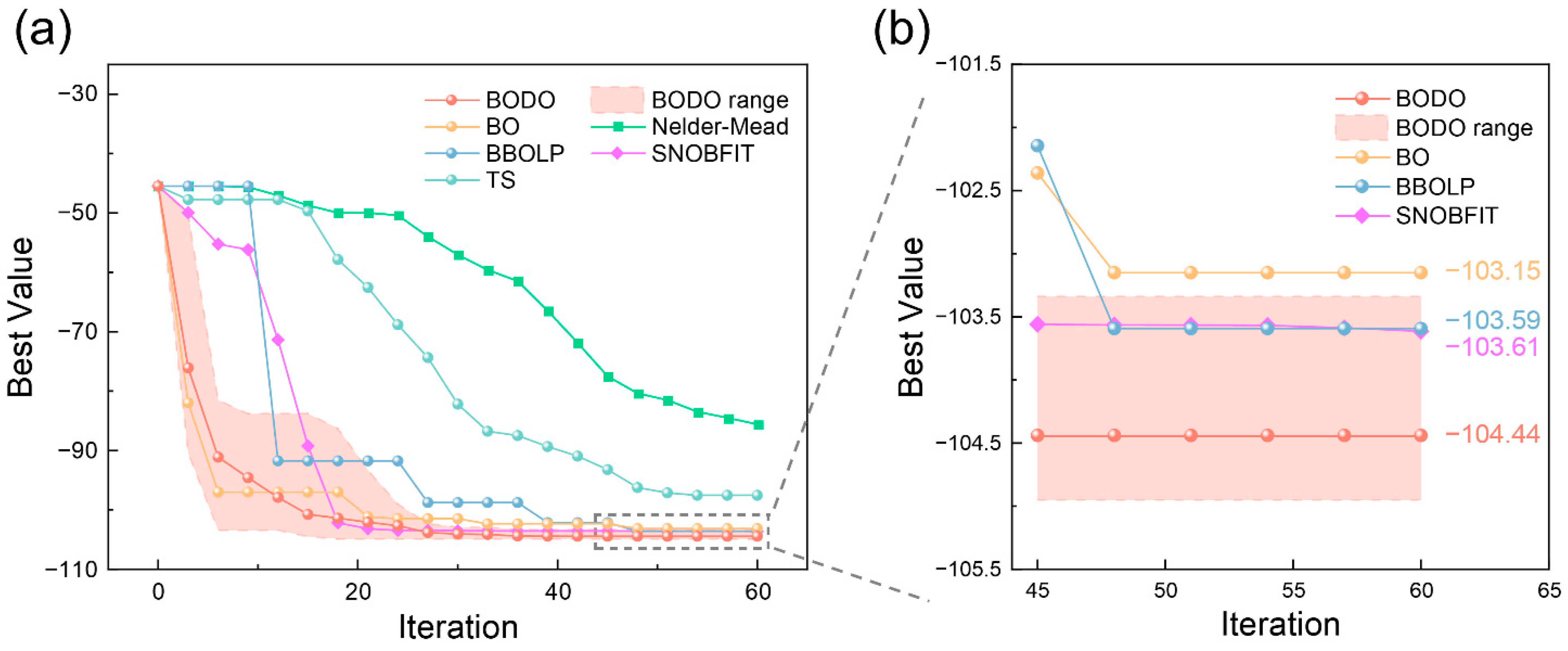
4.2. Benchmark Chemical Process: Summit SnAr

An open-source benchmark chemical process, Summit SnAr (Figure 7) is used to further test the proposed BODO and other methods for comparison [30,48]. Nucleophilic aromatic substitution reaction is a commonly used reaction in the fine chemical industry. The reaction condition optimization of the nucleophilic aromatic substitution reaction is of significant importance. In the Summit SnAr case, 2,4-dinitrofluorobenzene (1) undergoes nucleophilic attack by pyrrolidine (2) to form the desired product (3). The feedstock (1) and the product (3) can also react with (2) to form two side products, (4) and (5). Generally, the overall optimization target is to maximize the space–time yield of the designed product and minimize the side product production. Kinetic parameters of the four SnAr reactions are obtained from a previous report. Detailed pre-exponential factors and activation energies are listed in

Table 1. Pre-exponential factors and activation energies of Summit SnAr reactions.

Step	k (10−2·mol−1·s−1)	Ea (kJ·mol−1)
1	57.9 ± 0.7	33.3 ± 0.3
2	2.70 ± 0.06	35.3 ± 0.5
3	0.865 ± 0.004	38.9 ± 1.5
4	1.63 ± 0.11	44.8 ± 1.8

.

The SnAr reactions are simulated to occur in a plug flow reactor, for which the residence time, stoichiometry, and temperature can be adjusted. The descriptions and feasible domain ranges of input variables and output objectives are given in

Table 2. The input variables and objectives of Summit SnAr.

Name	Type	Description	Domain Range
$tau$	input	residence time	[0.5, 2]
$equ{i}_{pldn}$	input	equivalents of pyrrolidine	[1, 5]
$con{c}_{dfnb}$	input	concentration of 2,4-dinitrofluorobenenze	[0.1, 0.5]
$temperature$	input	reactor temperature	[30, 120]
$sty$	objective	space time yield (kg/m3/h)
$e_{factor}$	objective	weight ratio of product 4 and 5 over 3

.

Combining $sty$ and $e_{factor}$, the multi-objective optimization problem can be transformed into a single objective optimization problem with Equation (12), where $\alpha$ is a negative parameter to measure the weight between $sty$ and $e_{factor}$. Referring to the reported literature, $\alpha$ is set to −0.01 in this work (Felton et al., 2021). During optimization, a minus sign is added to the objective function to transform the optimization problem into a maximization one.

$$\min objective=\alpha \times sty+e_{factor}$$

(12)

The Summit SnAr test details are as follows: 12 random experiment points were selected by random sampling as the initial dataset, and all optimization algorithms were sequentially iterated for 60 rounds with the same initial point sets.

The optimization results are plotted in Figure 8. To exclude the influence of randomness, BODO was run for 10 times to obtain the average, as well as other non-deterministic algorithms (TS and SNOBFIT). Deterministic algorithms were applied without repetition. The minimal and maximal result values of BODO are also recorded at all iterations. Consistent with the results on alpine functions, BODO outstands from other methods in final best optimization value. In comparison, TS and Nelder–Mead displayed a slower convergence speed throughout the optimization iteration. Meanwhile, SNOBFIT also suffers from the sluggish optimization speed in the first 15 iteration rounds. Although the optimization speed of BO is competitive in the early optimization stage, its final best value (−103.15) is inferior to that of BODO (−104.44), which can be attributed to the exploration ability endowed by the D-optimal design branch. The final best values of BBOLP and SNOBFIT are −103.59 and −103.61, respectively, which are also better than BO, showing the importance of rational point distribution in the independent variable space. BBOLP is realized by local penalization, and SNOBFIT is realized by subregion division. Compared to BBOLP and SNOBFIT, BODO can directly sample points in the independent variable space according to the D-optimal design criterion and the final optimized best value is even better. Moreover, it is noteworthy that even the largest final best value (−103.34) of the 10 BODO runs is better than that of BO.

After experiment optimization, $tau$ and $con{c}_{dfnb}$ are both optimized to their corresponding range limits (both are optimized to 0.5). The $temperature$ and $equi{v}_{pldn}$ distributions of BO and BODO best solutions are shown in Figure 9. BO and 3 BODO best results are located near (1.5, 100), while the other seven best results of BODO are distributed within the contour line of −104.38, showing the effectiveness of BODO in experiment space exploration. Without profound knowledge of the experiment, BODO can recommend points based on optimal design and achieve a more rational sample distribution from an experiment design perspective. BODO delivers a balance between surrogate regression and D-optimal design, and can contribute to experiment optimization in the benchmark SnAr chemical process.

5. Conclusions

In this study, we developed an iterative optimization framework BODO to reduce the negative impact of poor initial point selection and local optimum on experiment optimization. BODO innovatively highlights the integration of BO in the dependent variable space search and D-optimal design in the independent variable space. BODO is designed to maintain the scaffold of BO for fast local convergence and involve stochasticity for D-optimal design to improve the global search ability. In addition, BODO integrates D-optimal design with BO by means of the probabilistic branch in each iteration, rather than only the initial point selection.

BODO is a flexible optimization framework that allows hyperparameters to be tuned according to actual requirements for fast convergence or a wide search range. BODO was shown to achieve better results than BO with repeated tests and different initial points in alpine2 test functions and the benchmark SnAr chemical process. A visualized 2-dimensional alpine2 function case shows BODO has a better global search ability by jumping out of the initial local optimum. Meanwhile, with the same number of iterations, BODO outperforms other typical optimization algorithms on alpine2 functions with different dimension sizes and the SnAr chemical process, exhibiting a competitive performance in terms of final best result and convergence speed, especially for processes with a relatively larger input dimension size. BODO balances between surrogate model-based exploitation and D-optimal design-based exploration to achieve a better experiment optimization performance. The proposed efficient BODO method is promising to be applied in chemical experiment optimization in the future, enlightening a new way for optimal condition search and experiment guidance.

References

1. Bourne, R.A.; Hii, K.K.; Reizman, B.J. Introduction to Synthesis 4.0: Towards an internet of chemistry. React. Chem. Eng. 2019, 4, 1504–1505. [Google Scholar] [CrossRef]
2. Mateos, C.; Nieves-Remacha, M.J.; Rincón, J.A. Automated platforms for reaction self-optimization in flow. React. Chem. Eng. 2019, 4, 1536–1544. [Google Scholar] [CrossRef]
3. Zhang, S.; Liang, X.; Huang, X.; Wang, K.; Qiu, T. Precise and fast microdroplet size distribution measurement using deep learning. Chem. Eng. Sci. 2021, 247, 116926. [Google Scholar] [CrossRef]
4. Clayton, A.D.; Manson, J.A.; Taylor, C.; Chamberlain, T.W.; Taylor, B.A.; Clemens, G.; Bourne, R.A. Algorithms for the self-optimisation of chemical reactions. React. Chem. Eng. 2019, 4, 1545–1554. [Google Scholar] [CrossRef]
5. Burger, B.; Maffettone, P.M.; Gusev, V.V.; Aitchison, C.M.; Bai, Y.; Wang, X.; Li, X.; Alston, B.M.; Li, B.; Clowes, R.; et al. A mobile robotic chemist. Nature 2020, 583, 237–241. [Google Scholar] [CrossRef]
6. Hughes, G.; Mills, H.; De Roure, D.; Frey, J.G.; Moreau, L.; Schraefel, M.C.; Smith, G.; Zaluska, E. The semantic smart laboratory: A system for supporting the chemical eScientist. Org. Biomol. Chem. 2004, 2, 3284–3293. [Google Scholar] [CrossRef] [Green Version]
7. Zendehboudi, S.; Ahmadi, M.A.; Mohammadzadeh, O.; Bahadori, A.; Chatzis, I. Thermodynamic Investigation of Asphaltene Precipitation during Primary Oil Production: Laboratory and Smart Technique. Ind. Eng. Chem. Res. 2013, 52, 6009–6031. [Google Scholar] [CrossRef]
8. Li, J.; Lu, Y.; Xu, Y.; Liu, C.; Tu, Y.; Ye, S.; Liu, H.; Xie, Y.; Qian, H.; Zhu, X. AIR-Chem: Authentic Intelligent Robotics for Chemistry. J. Phys. Chem. A 2018, 122, 9142–9148. [Google Scholar] [CrossRef]
9. Zhang, S.; Qin, K.; Huang, X.; Wei, Y.; Wang, T.; Wang, K.; Qiu, T. Insight into Microdispersion Flows with a Novel Video Deep Learning Method. Adv. Intell. Syst. 2022, 4, 2200098. [Google Scholar] [CrossRef]
10. Bi, K.; Zhang, S.; Zhang, C.; Li, H.; Huang, X.; Liu, H.; Qiu, T. Knowledge expression, numerical modeling and optimization application of ethylene thermal cracking: From the perspective of intelligent manufacturing. Chin. J. Chem. Eng. 2021, 38, 1–17. [Google Scholar] [CrossRef]
11. Hough, B.R.; Beck, D.A.; Schwartz, D.T.; Pfaendtner, J. Application of machine learning to pyrolysis reaction networks: Reducing model solution time to enable process optimization. Comput. Chem. Eng. 2017, 104, 56–63. [Google Scholar] [CrossRef] [Green Version]
12. Li, H.; Zhang, S.; Qiu, T. Two-Level Decoupled Ethylene Cracking Optimization of Batch Operation and Cyclic Scheduling. Ind. Eng. Chem. Res. 2022, 61, 16539–16551. [Google Scholar] [CrossRef]
13. Shields, B.J.; Stevens, J.; Li, J.; Parasram, M.; Damani, F.; Alvarado, J.I.M.; Janey, J.M.; Adams, R.P.; Doyle, A.G. Bayesian reaction optimization as a tool for chemical synthesis. Nature 2021, 590, 89–96. [Google Scholar] [CrossRef]
14. MacLeod, B.P.; Parlane, F.G.L.; Morrissey, T.D.; Häse, F.; Roch, L.M.; Dettelbach, K.E.; Moreira, R.; Yunker, L.P.E.; Rooney, M.B.; Deeth, J.R.; et al. Self-driving laboratory for accelerated discovery of thin-film materials. Sci. Adv. 2020, 6, eaaz8867. [Google Scholar] [CrossRef] [PubMed]
15. Gromski, P.S.; Henson, A.B.; Granda, J.M.; Cronin, L. How to explore chemical space using algorithms and automation. Nat. Rev. Chem. 2019, 3, 119–128. [Google Scholar] [CrossRef]
16. Häse, F.; Roch, L.M.; Aspuru-Guzik, A. Next-Generation Experimentation with Self-Driving Laboratories. Trends Chem. 2019, 1, 282–291. [Google Scholar] [CrossRef]
17. Ludl, P.O.; Heese, R.; Höller, J.; Asprion, N.; Bortz, M. Using machine learning models to explore the solution space of large nonlinear systems underlying flowsheet simulations with constraints. Front. Chem. Sci. Eng. 2021, 16, 183–197. [Google Scholar] [CrossRef]
18. Ma, Y.; Gao, Z.; Shi, P.; Chen, M.; Wu, S.; Yang, C.; Wang, J.; Cheng, J.; Gong, J. Machine learning-based solubility prediction and methodology evaluation of active pharmaceutical ingredients in industrial crystallization. Front. Chem. Sci. Eng. 2021, 16, 523–535. [Google Scholar] [CrossRef]
19. Zhou, Y.; Li, G.; Dong, J.; Xing, X.-H.; Dai, J.; Zhang, C. MiYA, an efficient machine-learning workflow in conjunction with the YeastFab assembly strategy for combinatorial optimization of heterologous metabolic pathways in Saccharomyces cerevisiae. Metab. Eng. 2018, 47, 294–302. [Google Scholar] [CrossRef]
20. Burre, J.; Kabatnik, C.; Al-Khatib, M.; Bongartz, D.; Jupke, A.; Mitsos, A. Global flowsheet optimization for reductive dimethoxymethane production using data-driven thermodynamic models. Comput. Chem. Eng. 2022, 162. [Google Scholar] [CrossRef]
21. Khamparia, A.; Pandey, B.; Pandey, D.K.; Gupta, D.; Khanna, A.; de Albuquerque, V.H.C. Comparison of RSM, ANN and Fuzzy Logic for extraction of Oleonolic Acid from Ocimum sanctum. Comput. Ind. 2020, 117, 103200. [Google Scholar] [CrossRef]
22. Aslan, V.; Eryilmaz, T. Polynomial regression method for optimization of biodiesel production from black mustard (Brassica nigra L.) seed oil using methanol, ethanol, NaOH, and KOH. Energy 2020, 209, 118386. [Google Scholar] [CrossRef]
23. Stuke, A.; Todorović, M.; Rupp, M.; Kunkel, C.; Ghosh, K.; Himanen, L.; Rinke, P. Chemical diversity in molecular orbital energy predictions with kernel ridge regression. J. Chem. Phys. 2019, 150, 204121. [Google Scholar] [CrossRef] [PubMed] [Green Version]
24. Antti, H.; Ebbels, T.M.; Keun, H.C.; Bollard, M.E.; Beckonert, O.; Lindon, J.C.; Nicholson, J.K.; Holmes, E. Statistical experimental design and partial least squares regression analysis of biofluid metabonomic NMR and clinical chemistry data for screening of adverse drug effects. Chemom. Intell. Lab. Syst. 2004, 73, 139–149. [Google Scholar] [CrossRef]
25. Olson, M.; Wyner, A.J.; Berk, R. Modern neural networks generalize on small data sets. In Proceedings of the 32nd International Conference on Neural Information Processing Systems; Curran Associates Inc.: Red Hook, NY, USA, 3 December 2018; pp. 3623–3632. [Google Scholar]
26. Zhang, S.; Liu, H.-X.; Gao, D.-T.; Wang, W. Surveying the methods of improving ANN generalization capability. In Proceedings of the 2003 International Conference on Machine Learning and Cybernetics, Xi’an, China, 5 November 2003; pp. 1259–1263. [Google Scholar] [CrossRef]
27. Shahriari, B.; Swersky, K.; Wang, Z.; Adams, R.P.; de Freitas, N. Taking the Human Out of the Loop: A Review of Bayesian Optimization. Proc. IEEE 2015, 104, 148–175. [Google Scholar] [CrossRef] [Green Version]
28. Cao, L.; Russo, D.; Felton, K.; Salley, D.; Sharma, A.; Keenan, G.; Mauer, W.; Gao, H.; Cronin, L.; Lapkin, A.A. Optimization of Formulations Using Robotic Experiments Driven by Machine Learning DoE. Cell Rep. Phys. Sci. 2021, 2, 100295. [Google Scholar] [CrossRef]
29. Fantke, P.; Cinquemani, C.; Yaseneva, P.; De Mello, J.; Schwabe, H.; Ebeling, B.; Lapkin, A.A. Transition to sustainable chemistry through digitalization. Chem 2021, 7, 2866–2882. [Google Scholar] [CrossRef]
30. Felton, K.C.; Rittig, J.G.; Lapkin, A.A. Summit: Benchmarking Machine Learning Methods for Reaction Optimisation. Chem 2021, 1, 116–122. [Google Scholar] [CrossRef]
31. Nguyen, V.; Rana, S.; Gupta, S.K.; Li, C.; Venkatesh, S. Budgeted Batch Bayesian Optimization. In Proceedings of the 2016 IEEE 16th International Conference on Data Mining (ICDM), Barcelona, Spain, 12–15 December 2016; pp. 1107–1112. [Google Scholar] [CrossRef]
32. Sun, S.; Tiihonen, A.; Oviedo, F.; Liu, Z.; Thapa, J.; Zhao, Y.; Hartono, N.T.P.; Goyal, A.; Heumueller, T.; Batali, C.; et al. A data fusion approach to optimize compositional stability of halide perovskites. Matter 2021, 4, 1305–1322. [Google Scholar] [CrossRef]
33. Xue, D.; Balachandran, P.V.; Yuan, R.; Hu, T.; Qian, X.; Dougherty, E.R.; Lookman, T. Accelerated search for BaTiO 3 -based piezoelectrics with vertical morphotropic phase boundary using Bayesian learning. Proc. Natl. Acad. Sci. USA 2016, 113, 13301–13306. [Google Scholar] [CrossRef] [Green Version]
34. Jorayev, P.; Russo, D.; Tibbetts, J.D.; Schweidtmann, A.M.; Deutsch, P.; Bull, S.D.; Lapkin, A.A. Multi-objective Bayesian optimisation of a two-step synthesis of p-cymene from crude sulphate turpentine. Chem. Eng. Sci. 2021, 247, 116938. [Google Scholar] [CrossRef]
35. Pukelsheim, F. Optimal Design of Experiments, Classics in Applied Mathematics; Society for Industrial and Applied Mathematics: Philadelphia, PA, USA, 2006. [Google Scholar] [CrossRef] [Green Version]
36. Močkus, J. On bayesian methods for seeking the extremum. In Optimization Techniques IFIP Technical Conference; Marchuk, G.I., Ed.; Springer: Berlin/Heidelberg, Germany, 1975; pp. 400–404. [Google Scholar] [CrossRef] [Green Version]
37. Fisher, R.A. Design of Experiments. Br. Med. J. 1936, 1, 554. [Google Scholar] [CrossRef]
38. Baumgartner, L.M.; Coley, C.W.; Reizman, B.J.; Gao, K.W.; Jensen, K.F. Optimum catalyst selection over continuous and discrete process variables with a single droplet microfluidic reaction platform. React. Chem. Eng. 2018, 3, 301–311. [Google Scholar] [CrossRef] [Green Version]
39. Cox, D.; Reid, N. The Theory of the Design of Experiments; Chapman and Hall/CRC: Boca Raton, FL, USA, 2000. [Google Scholar] [CrossRef]
40. de Aguiar, P.; Bourguignon, B.; Khots, M.; Massart, D.; Phan-Than-Luu, R. D-optimal designs. Chemom. Intell. Lab. Syst. 1995, 30, 199–210. [Google Scholar] [CrossRef]
41. Kuram, E.; Ozcelik, B.; Bayramoglu, M.; Demirbas, E.; Simsek, B.T. Optimization of cutting fluids and cutting parameters during end milling by using D-optimal design of experiments. J. Clean. Prod. 2013, 42, 159–166. [Google Scholar] [CrossRef]
42. Gonzalez, J.; Dai, Z.; Hennig, P.; Lawrence, N. Batch Bayesian Optimization via Local Penalization. In Proceedings of the 19th International Conference on Artificial Intelligence and Statistics, Cadiz, Spain, 9–11 May 2016; pp. 648–657. [Google Scholar]
43. Frazier, P.I. Bayesian optimization, in: Recent Advances in Optimization and Modeling of Contemporary Problems. Informs 2018, 11, 255–278. [Google Scholar]
44. Schulz, E.; Speekenbrink, M.; Krause, A. A tutorial on Gaussian process regression: Modelling, exploring, and exploiting functions. J. Math. Psychol. 2018, 85, 1–16. [Google Scholar] [CrossRef]
45. Bradford, E.; Schweidtmann, A.M.; Lapkin, A. Efficient multiobjective optimization employing Gaussian processes, spectral sampling and a genetic algorithm. J. Glob. Optim. 2018, 71, 407–438. [Google Scholar] [CrossRef] [Green Version]
46. Cortés-Borda, D.; Kutonova, K.V.; Jamet, C.; Trusova, M.E.; Zammattio, F.; Truchet, C.; Rodriguez-Zubiri, M.; Felpin, F.-X. Optimizing the Heck–Matsuda Reaction in Flow with a Constraint-Adapted Direct Search Algorithm. Org. Process. Res. Dev. 2016, 20, 1979–1987. [Google Scholar] [CrossRef] [Green Version]
47. Huyer, W.; Neumaier, A. SNOBFIT—Stable Noisy Optimization by Branch and Fit. ACM Trans. Math. Softw. 2008, 35, 1–25. [Google Scholar] [CrossRef]
48. Hone, C.A.; Holmes, N.; Akien, G.R.; Bourne, R.A.; Muller, F.L. Rapid multistep kinetic model generation from transient flow data. React. Chem. Eng. 2016, 2, 103–108. [Google Scholar] [CrossRef] [PubMed]
Figure 1. Diagram of BODO framework.
Processes 11 00087 g001
Figure 2. Visualized optimization processes of BO (a) and BODO (b) on the 2-dimensional alpine2 function (alpine22d) with the same preset bad-quality initial points. The hyperparameters ε 1 , ε 2 , and β are set to 0.6, 0.4, and 0.95, respectively. Points of different iteration segments are indicated with different colors.
Processes 11 00087 g002
Figure 3. The average optimization results on alpine25d. (ae) The heatmap of best values of BODO with different ε 1 and ε 2 settings at iterations 10, 20, 30, 40, and 50, respectively. (f) The best value comparison of BODO ( ε 1 = 0.6 , ε 2 = 0.4 ) with its counterparts that include only the LP D-optimal branch ( ε 1 = 0.6 , ε 2 = 1.0 ), only the random selection D-optimal branch ( ε 1 = 0.6 , ε 2 = 0.0 ), and no D-optimal branch ( ε 1 = 0.0 ).
Processes 11 00087 g003
Figure 4. (a) BODO and BO optimization results with 10 different random initial point sets, with BO results and BODO average results noted. (b) Example iteration processes of BODO and BO with the initial point 7.
Processes 11 00087 g004
Figure 5. The average BODO performance with different β settings (1.00, 0.98, 0.95, 0.90, and 0.85) on (a) alpine23d, (b) alpine25d, and (c) alpine28d test functions. BODO is run for 10 times over 10 random initial point sets. The initial point sets are the same for all β settings.
Processes 11 00087 g005
Figure 6. Average optimization results of BODO ( ε 1 = 0.6 ,   ε 2 = 0.4 ,     β = 1 ) and comparing algorithms on (a) alpine23d, (b) alpine25d, and (c) alpine28d test functions. Their theoretical minimal values are −17.21, −135.73, and −3005.58, respectively. Algorithms are run for 80, 120, and 200 iterations on alpine23d, alpine25d, and alpine28d, respectively. The average results are obtained from 10 random initial point sets which are set the same for all algorithms. Non-deterministic methods (BODO, TS, and SNOBFIT) are run for 10 times on each initial point set and then the results are averaged. The batch size of BBOLP is set to 5.
Processes 11 00087 g006
Figure 7. Chemical reactions of the Summit SnAr benchmark chemical process.
Processes 11 00087 g007
Figure 8. Optimization results of BODO and comparing algorithms on Summit SnAr. (a) average optimization results of different algorithms and BODO distribution range at each iteration. Non-deterministic algorithms (BODO, TS, and SNOBFIT) are run for 10 times. (b) Enlarged optimization results in the last few iterations. The batch size of BBOLP is set to 3.
Processes 11 00087 g008
Figure 9. The best result distribution of BO and 10 random BODO runs on t e m p e r a t u r e and e q u i v p l d n . For BO and all BODO runs, t a u and c o n c d f n b are all optimized to their boundaries, with their optimized values as 0.5 and 0.5, respectively.
Processes 11 00087 g009