Gas Pipeline Flow Prediction Model Based on LSTM with Grid Search Parameter Optimization

Abstract

Due to the abundant operation data (e.g., pressure, flow rate, and temperature) for natural gas (NG) gathering pipelines provided by the supervisory control and data acquisition (SCADA) system, the machine-learning-based real-time flow prediction has become a critical solution to enable the identification of the abnormality of pipelines, further to guarantee the safe operation of the pipelines. However, traditional machine-learning-based methods cannot always function well due to the temporal characteristics of the SCADA data often being ignored, resulting from a lack of time memory capability. Therefore, this paper proposes a method to automatically perform the feature mining of flow time series by considering the correlation of flow data at both ends of the pipeline, combined with the long short-term memory (LSTM) network. The current and historical data at both pipeline ends are used as input vectors of the LSTM network to predict the terminal output flow at the next moment. Furthermore, to solve the problem that the parameters of the LSTM model are configured with manual experience, a grid search algorithm (GSA) is introduced to optimize the parameters of the LSTM. Consequently, the effectiveness and superiority of the proposed method are carried out in a real-world NG gathering pipeline.

1. Introduction

According to the research published by the transportation research board (TRB) in 2004 [1], pipeline transmission is the safest way in the natural gas (NG) transmission area, but it does not mean that they are at zero risk. In China, NG pipelines will enter a highly aging stage in the next ten to twenty years, and pipeline accidents will also occur frequently over time [2]. Therefore, guaranteeing the reliability of NG pipeline transmissions has become an urgent demand for energy sectors [3,4]. Currently, supervisory control and data acquisition (SCADA) systems are widely applied in the NG pipelines for real-time observation of pipeline state variables [5,6,7]. However, real-time data of pipeline SCADA systems cannot be effectively mined and leveraged. Assuming that the pipeline flow can be obtained in advance by mining SCADA data, the real-time tracking of the pipeline operation can be realized to help the operator judge the abnormal condition and formulate a responding operation scheme. Thus, it is necessary to estimate the flow state of NG pipelines.

Till now, some monitoring techniques, which build fluid models in pipelines based on the conservation of mass, momentum, and energy, are proposed to monitor pipeline flow [8,9]. However, the analytical model of NG pipelines is difficult to establish due to the mass of state variables and the complexity of physical process knowledge. Fortunately, the artificial neural network (ANN) provides an alternative solution to describe the complex industrial system because of the advantage of approximate arbitrary nonlinear mappings. For example, Mounce et al. integrated a fuzzy inference system (FIS) and ANN to detect pipeline bursts, where abundant history data are utilized for training the ANN model to predict the urban water supply pipeline flow, and the FIS is used for detecting abnormalities [10]. Nevertheless, this method requires an amount of data for model training, and ANN training is time-consuming, which is easy to cause untimely alarm.

Moreover, some issues that exist in traditional prediction methods are as follows: (1) the model prediction accuracy highly relies on the design of the feature extraction method, while it always requires in-depth expert knowledge; (2) it is difficult to guarantee that the complex process dynamic characteristics can be fully exhibited by using expert knowledge for feature extraction [11]; and (3) using the existing machine learning models (such as support vector machine and ANN), it is hard to obtain enough features due to the use of the shallow network. In the context of big data, it is accompanied by great computational burden and modeling complexity, which leads to the traditional machine learning methods being unable to be satisfied with the application of the pipeline data prediction. By contrast, data-driven methods with deep learning (DL) obtained more attention because they can automatically and effectively perform statistical analysis and information extraction on massive, multi-source, and high-dimensional data [12].

Although DL performs a strong ability to extract features, there are also several challenges with the feature extraction of the NG pipeline data. Firstly, the SCADA data of the NG pipeline are non-linear and fluctuating. Time series data mining temporal characteristics effectively from the SCADA data is the premise of obtaining accurate predictions for the pipeline flow [13]. To handle the problem, the long short-term memory (LSTM) network, which is a member of DL algorithms that can fully explore the temporal characteristics of time series data, is adopted in this work. Specifically, LSTM can use the gate control mechanism on the internal memory cell to learn and represent the long-term dependence between the input sequence data (i.e., LSTM networks can remember the past time series information). Hence, it is suitable for feature learning on the time series data.

Secondly, the parameters of the neural network (NN) should be pre-assigned before the model trains, which determines the structure of the NN and further affect the computational burden of model training and prediction. Thus, the parameter optimization of the model is an important guarantee of the excellent performance of the model. However, LSTM is similar to other DL networks in the difficulty of the parameter selection and often relies on the hand-engineered adjustment. Manual parameter adjustment is difficult, especially in the context of massive data and complex deep network structures. In order to obtain the optimal parameters combination of LSTM to construct an appropriate model structure and improve the prediction accuracy of the LSTM model for NG pipeline flow, a grid search algorithm (GSA) is introduced to search for the optimal parameters for the LSTM model. Finally, a GSA-based LSTM (GSA-LSTM) model is proposed for predicting the NG pipeline flow.

The main contributions of this work can be summarized as follows:

(1)

A pipeline flow prediction scheme via LSTM is proposed to accurately estimate the NG pipeline flow by incorporating temporal correlations in the SCADA data.

(2)

A GSA optimization method is introduced to automatically search for the optimal parameter combination for the LSTM model, which solves the drawback of traditional hand-engineered selection.

(3)

Thorough investigations of GSA-LSTM based on a real-life NG pipeline are reported, which would provide good instruction for NG pipeline condition monitoring.

The remainder of this paper is structured as follows. Section 2 briefly introduces the long short-term memory (LSTM) network. The framework of the proposed GSA-LSTM model is presented in Section 3. In Section 4, the performance of GSA-LSTM is verified by a real-life NG gathering pipeline. Section 5 concludes the work.

2. Brief Revisit of Long Short-Term Memory Network

The long short-term memory (LSTM) network is a special recurrent neural network (RNN) model for widely enjoying time series prediction tasks, which is developed to handle the issues of gradient disappearance and the explosion of the RNN [14,15]. Different from only learning input point-to-output point mapping relationships of other conventional machine learning methods, LSTM can retain the time dependencies of long sequences data. In addition, as a nonlinear model, LSTM can be used as a complex nonlinear element to construct a stronger network prediction model. Considering the nonlinearity and time dependencies of pipe operation SCADA data, the LSTM is utilized as the baseline of the pipeline flow prediction model in this work.

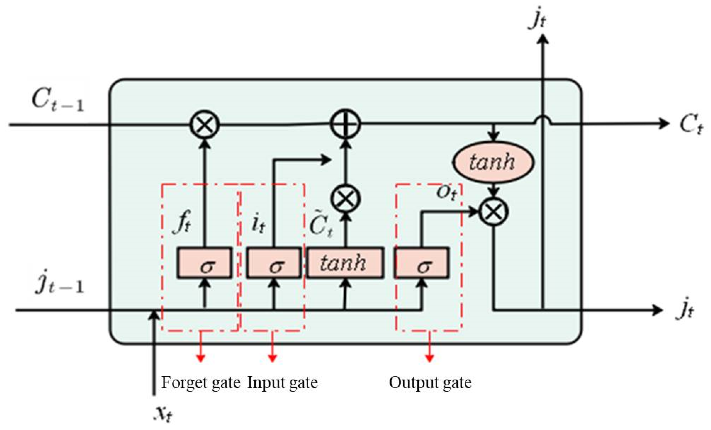
Generally, a basic LSTM unit structure includes the forget gate, the input gate, and the output gate, as shown in Figure 1. Among these gate control cells, the forget gate determines what information from the previous time step and the current input should be discarded or retained, and the input gate and the output gate are used to update the cell status and control the information to be passed to the next LSTM unit, respectively. The update expression of LSTM stored cells in step t can be formulated as follows:

$$f_t=\sigma \left(W_f{x}_t+U_f{j}_{t-1}+b_f\right)$$

(1)

$$i_t=\sigma \left(W_i{x}_t+U_i{j}_{t-1}+b_i\right)$$

(2)

$$o_t=\sigma \left(W_o{x}_t+U_o{h}_{t-1}+b_o\right).$$

(3)

$$\overline{C_t}=\tanh \left(W_c{x}_t+U_c{j}_{t-1}+b_c\right)$$

(4)

$$c_t=f_t\mathrm{e}{c}_{t-1}+i_t\overline{c_t}$$

(5)

$$h_t=o_t\mathrm{e}\mathrm{Tanh}\left(c_t\right)$$

(6)

where $\sigma$ is the sigmoid activation function, $j_{t-1}$ denotes the information from the previous hidden state, $x_t$ is the current input, $W_f$, $U_f$, $W_i$, $U_i$, $W_o$, $U_o$, $W_c$ and $U_c$ are represent the corresponding weight matrix, respectively, and $f_f$, $f_i$, $f_o$, and $f_c$ are bias term, respectively, they are updated with the learning process of the network.

3. Framework of the Proposed GSA-LSTM for NG Pipeline Flow Prediction

In this work, to realize the high-accuracy prediction of the NG pipeline flow by fully exploring the useful information in the SCADA data, a grid search parameter optimization-based LSTM model is proposed. The details of the proposed pipeline flow prediction method will be discussed in the following sections.

3.1. Data Acquisition and Preprocessing

In modern gas and oil companies, almost all the NG gathering pipelines are equipped with a SCADA system to collect real-time time series signals, such as the flow, pressure, and temperature. In this work, the continuous time series signals, including the flow, and pressure, are used to build the healthy pipeline flow prediction model. Nevertheless, the flow prediction accuracy of the NG pipeline highly depends on the quality of SCADA data [16]. In fact, although the system is under normal working conditions, due to the influence of the objective environment and the collection device, the continuous monitoring data show the characteristics of the fixed frequency and variable amplitude. As a result, the SCADA data collected at the output end of the pipeline may be missing or abnormal, which will further lead to fracture on the timescale and reduce model prediction accuracy. Therefore, it is necessary to preprocess SCADA data before constructing the prediction model.

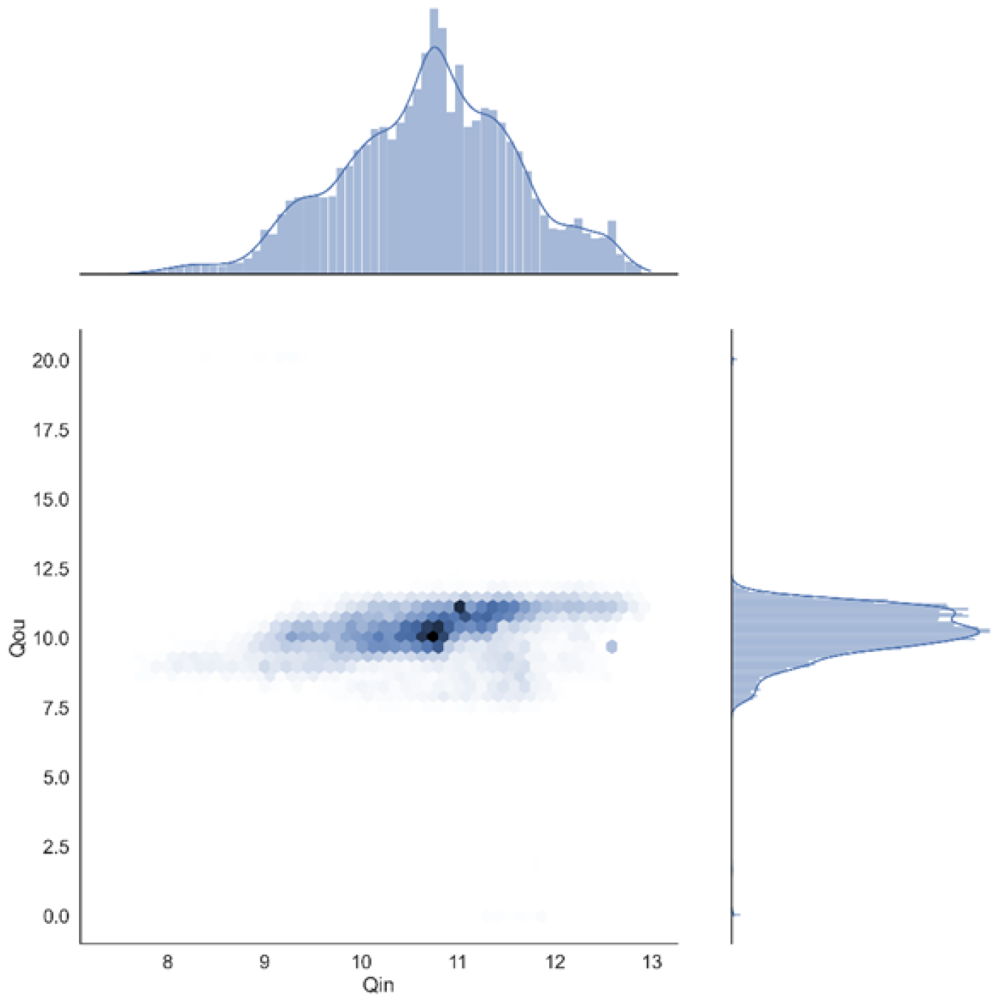
Specifically, Figure 2 shows the distribution density plot of flow at the input and output ends of the NG pipeline, where the shaded part of the hexagon is the joint density distribution of the pipeline input and output flow. The outer parts are the distribution histogram of the flow at the pipeline input $Q_{in}$ and output $Q_{ou}$, respectively, which present the normal distribution. 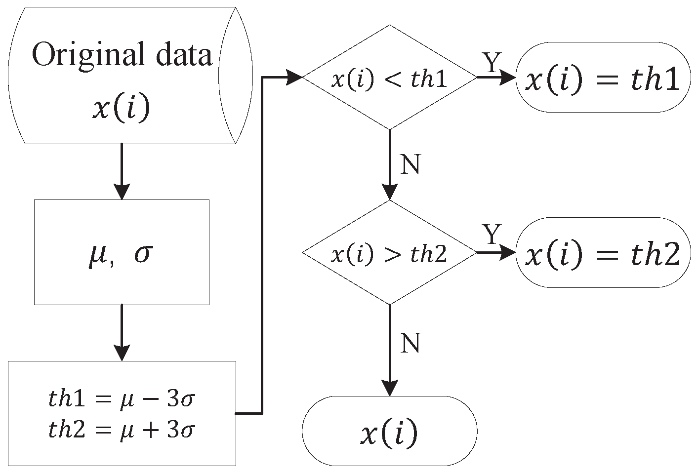According to the data distribution characteristics, the $3\sigma$ criterion is employed to eliminate maximum outliers in this work. The procedure of the data preprocessing is illustrated in Figure 3, where $\sigma$ and $\mu$ are the standard deviations and mean value of the original data $x\left(i\right)$, respectively.

3.2. Procedure of LSTM Based NG Pipeline Flow Prediction

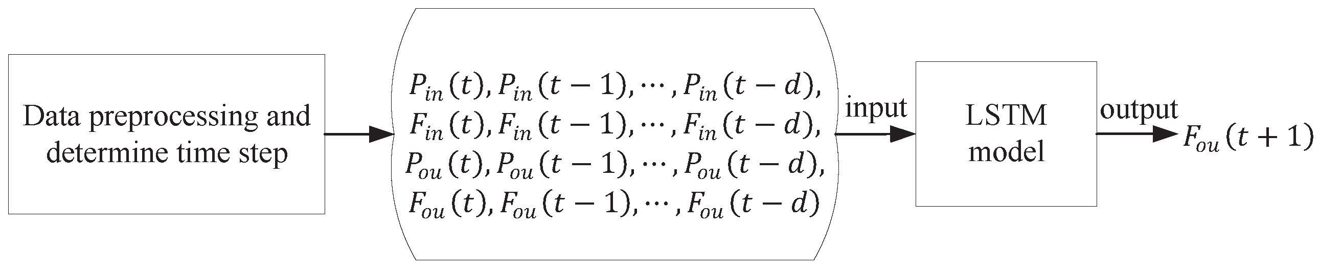
The DL-based method has been well-accepted to solve the problem that it is difficult to establish accurate mechanism models in process industries [17], the non-linear activation functions (e.g., sigmoid) and two-layer weighted network can approximate any mechanism process with high accuracy [18,19]. In this paper, considering the temporal features of the SCADA data and the advantage of the LSTM model in time series data modeling, we first take the continuous time series data of a specified length adjacent to the target timestamp as the model input, where the temporal features of the data can be extracted by the recurrent structure of the LSTM model, and further predict the corresponding value of the target timestamp. The traditional prediction models are only constructed using the single state at the pipe end, which always performs poorly. However, the NG gathering pipeline is a complex system with continuous change, and there is a high correlation between the pipeline operation states. Therefore, the historical input and output ends of the NG pipeline pressure (P) and flow (F) are utilized to predict the output flow of the next time step and the difference between the actual and predicted output flow (i.e., residual) as the evaluation index of the pipeline operation condition.

As illustrated in Figure 4, the implementation procedure of the LSTM-based NG pipeline flow prediction can be specifically split as follows:

Step 1: Preprocess the time series data collected by the SCADA system through the method described in Section 3.1 to obtain high-quality data.

Step 2: Utilize a sliding window to segment the original pipeline state data into many subsequences with the same length, where the sliding size is set as 1. Given a known data sequence $q_1,q_2,\dots ,q_n$, the $q_{k+1}$ is the output label of the subsequence $q_1,q_2,\dots ,q_n$, when the sequence length is set as k, while $q_{k+2}$ is the label of $q_2,q_3,\dots ,q_{k+1}$. By analogy, the model required input data with the size of $n-k+1$ is finally constructed, and further split into training and testing sets.

Step 3: Train LSTM by using the training set, then the LSTM-based pipeline flow prediction model can be described as follows:

$$F_{ou}(t+1)=NN\left[\begin{array}{c}{P}_{in}\left(t\right),P_{in}(t-1),\dots ,P_{in}(t-d)\\ F_{in}\left(t\right),F_{in}(t-1),\dots ,F_{in}(t-d)\\ P_{ou}\left(t\right),P_{ou}(t-1),\dots ,P_{ou}(t-d)\\ F_{ou}\left(t\right),F_{ou}(t-1),\dots ,F_{ou}(t-d)\end{array}\right]$$

(7)

where the $F_{ou}(t+1)$ is the predicted flow at the pipeline output, $P_{in}$ and $P_{ou}$ represent the pressure at the input and output ends of the pipeline, respectively, while $F_{in}$ and $F_{ou}$ are the pipeline input and output flow, respectively, d is the time sequence length, and $NN[\ast ]$ denotes the LSTM network. For each test datum, the corresponding predicted flow can be obtained according to Equation (7).

3.3. GSA-Based Parameter Optimization Strategy for LSTM

The model parameters of traditional NN networks are commonly determined by the manual-experience selection, which is difficult to find proper parameters to make the model perform well. In this work, the grid search algorithm (GSA) is used to solve the problem of traditional parameter selection. GSA is a well-adopted exhaustive optimization method, which can find the optimal solution for the objective problem by using exhaustive grid search in the given search range, thereby providing the relative best modeling parameters for the LSTM. In detail, the main steps of GSA optimization-based LSTM pipeline flow prediction are outlined as follows:

Step 1: Determine the search range of LSTM modeling parameters and deliver them to the grid search function to arrange all combinations in the given range.

Step 2: Construct different LSTM models based on each parameter combination.

Step 3: Define the loss function to evaluate the performance of model parameters, mean square error (MSE) is used as the loss function in this work:

$$J_{LOSS}=\frac{1}{n}\sum _{i=1}^{n}L(y_i,\widehat{y_i})=\frac{1}{n}\sum _{i=1}^n{(y_i-\widehat{y_i})}^2$$

(8)

where $L(·)$ denotes the loss function, n is the sample size, and $y_i$ and $\widehat{y_i}$ are the actual and predicted output of the ith sample, respectively.

Step 4: Obtain the final values of the loss function for each LSTM model after the network training reaches the maximum learning iteration.

Step 5: The best solution with the lowest loss function value is chosen to provide the optimal parameter combination for LSTM modeling.

4. Experiments

In this section, the proposed pipeline flow prediction model GSA-LSTM is evaluated through applications to a real-world NG gathering pipeline system in Nanchong, China. The prediction performance of the proposed method is evaluated using the root mean square error (RMSE) and mean absolute percentage error (MAPE):

$$\mathrm{RMSE}=\sqrt{\frac{1}{n_{test}}{\displaystyle \sum _{i=1}^{n_{test}}}{({\widehat{y}}_{test,i}-y_{test,i})}^2}$$

(9)

$$\mathrm{MAPE}=\sum _{i=1}^{n_{test}}|\frac{{\widehat{y}}_{test,i}-y_{test,i}}{y_{test,i}}|\times \frac{100}{n_{test}}$$

(10)

where $n_{test}$ is the number of query samples, and $y_{test,i}$ and ${\widehat{y}}_{test,i}$ are the observed and predicted values of the ith sample, respectively. The smaller the value of the RMSE and MAPE, the higher the prediction accuracy of the model.

4.1. Dataset Description

The experiment dataset was collected from the SCADA data of the healthy NG pipeline provided by the Longgang gas field, and the sampling interval is 20 seconds. The data from 28 February 2020 to 7 March 2020 were collected, where the data from 28 February 2020 to 5 March 2020 are used for model training while the remaining data are used for testing.

Table 1. Instances of the collected data of pipeline input and output ends.

Time	Input Pressure	Input Flow	Output Pressure	Output Flow
2020-02-28 14:33:00	6.20	8.66	6.05	8.58
2020-02-28 14:33:20	6.20	8.75	6.05	8.70
2020-02-28 14:33:40	6.20	8.72	6.05	8.55
2020-02-28 14:34:00	6.20	8.07	6.05	8.32

shows some instances of the collected data of both pipeline ends; there are a total of four variables including the pipeline input and output pressure and flow.

To eliminate the scale influence between variables, it is necessary to normalize the variables after the data preprocessing mentioned in Section 3.1. In this paper, the min-max scaling method is utilized to map the original data to the range of $[0,1]$, and realize the equal scaling of the original data. The normalization formula is as follows:

$$X_{norm}=\frac{X-X_{min}}{X_{max}-X_{min}}$$

(11)

where X is the original data, $X_{max}$ and $X_{min}$ are the maxim and minimal value in the X, $X_{norm}$ is the normalized data. Subsequently, a sliding window is used to divide the original data sequence into many subsequences to satisfy the input requirement of the proposed method.

4.2. Model Parameters Optimization

To obtain high-accuracy prediction model, four critical parameters (learning rate, bacth size, time sequence length, and the number of hidden layer nodes) for the LSTM method are optimized by the GSA. The candidates for these parameters are tabulated in

Table 2. The candidates for modeling parameters.

No.	Parameter Type	Candidate Range
1	Learning rate (lr)	$0.1,0.01,0.001$
2	Time sequence length (L)	3~30
3	The number of hidden layer nodes (n)	8~128
4	Batch size	16~51

, and the details of the parameters optimization are analyzed in the following subsections.

a.

Learning rate

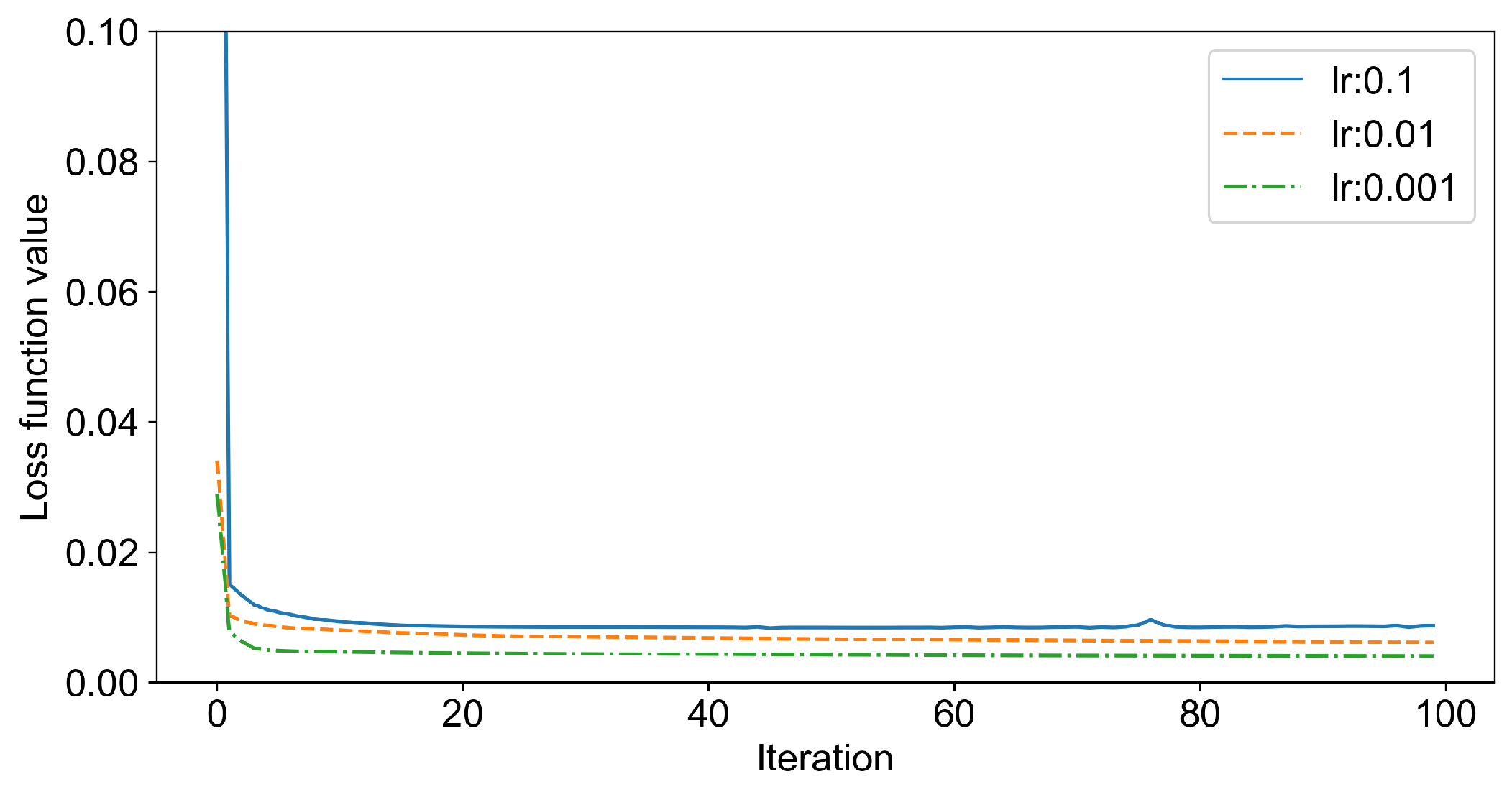
The learning rate is the speed of information accumulation with the process of the NN training, which determines whether the loss function of the NN can effectively converge to the optimal value. In the process of parameters optimization, the loss reduction of the loss function under the different learning rates is shown in Figure 5. It can be seen that when the learning rate is set as $0.001$, the minimum training loss is obtained. The converging speed of the built LSTM is fast, as the loss function converges rapidly within 20 iterations.

b.

Batch size

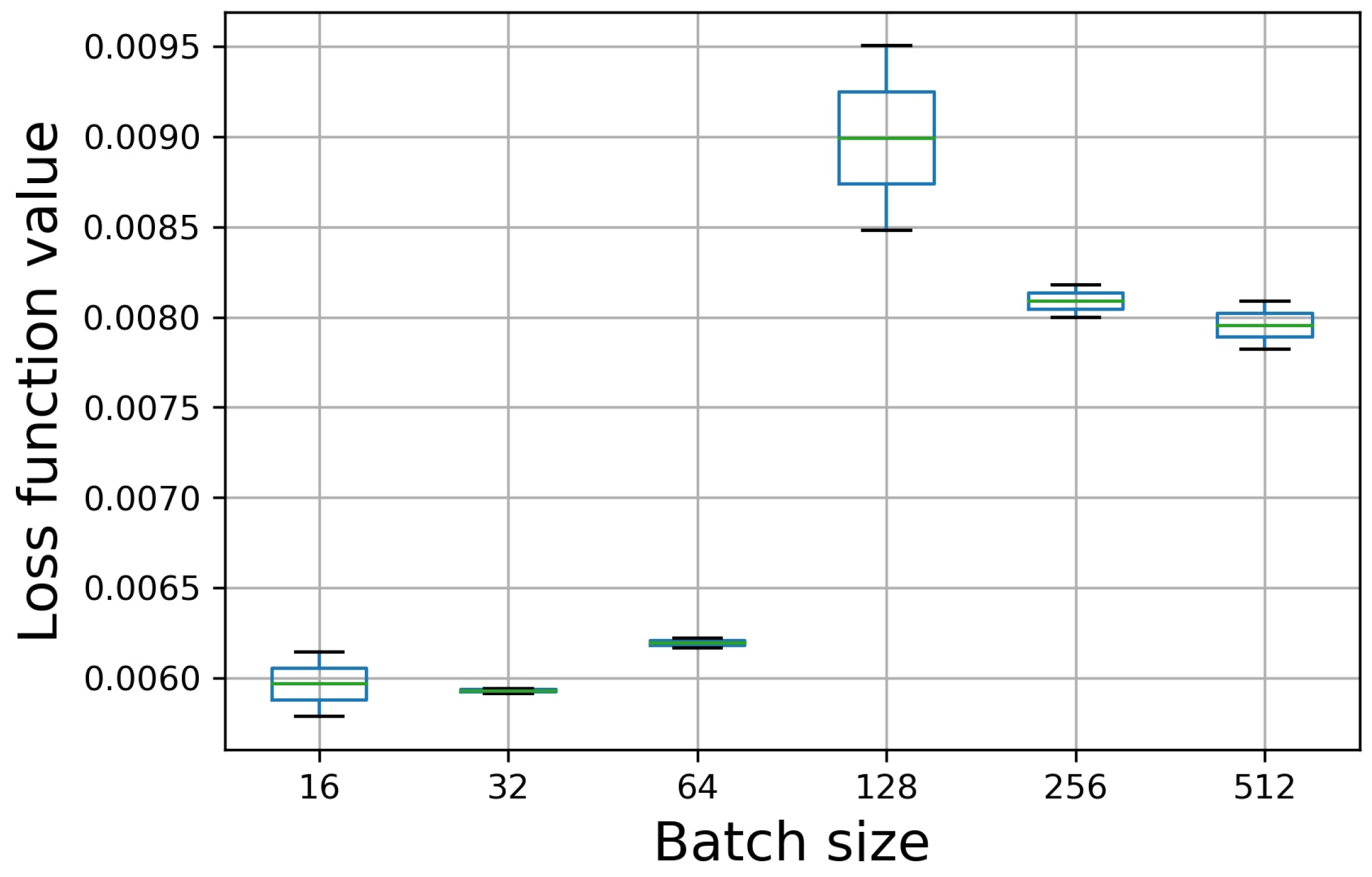
The number of samples selected for each training; batch size affects the memory usage and the model’s optimization degree and speed. The batch size is too small, which may cause difficulty in model convergence. The batch size is too large. Although the training time can be reduced, the model’s generalization performance will decline as the required memory capacity increases. This paper comprehensively considers the amount of data, calculates the cost and time cost, and the search range of batch size set as 16 to 512. Figure 6 shows the loss functional value under different batch sizes. The GSA algorithm in this paper uses mean squared error as the loss function. The smaller the MSE value, the better the performance of this version of the model. It can be seen from the figure that when the batch size is 32, the mean value of the mean squared error is the smallest, and the confidence interval is the smallest, which means that the model performance is the most stable at this time.

c.

Time sequence length

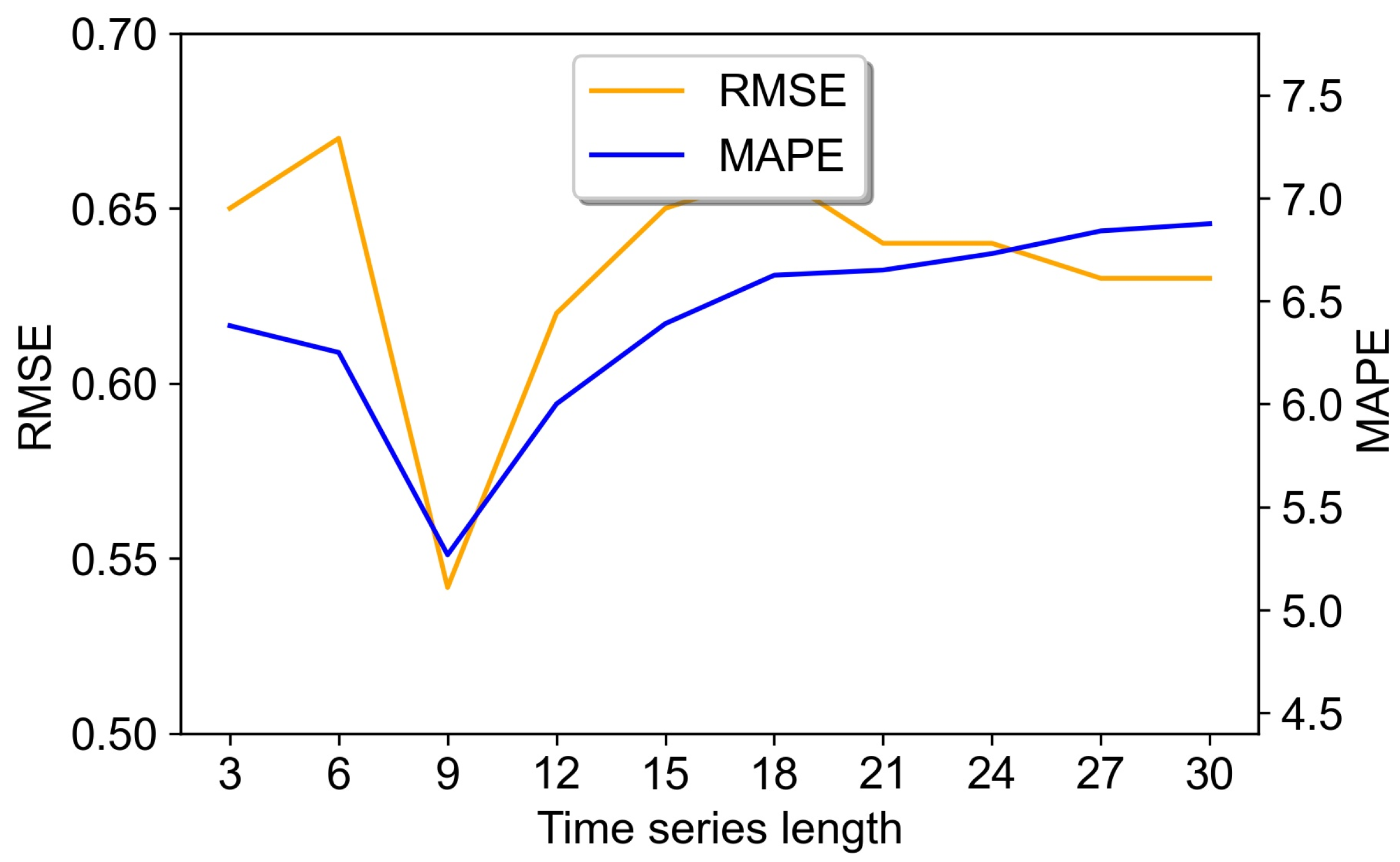
The different time sequence length has a great impact on the performance of the NN model [20]; a too-short sequence cannot fully leverage the capability of LSTM for processing time series data, while a too-long sequence will increase the modeling complexity, even against the model prediction performance. Consequently, the time sequence length is chosen as the key to optimized model parameters in this work. Figure 7 shows the influence of different sequence lengths on the model prediction accuracy, it is readily observed that the RMSE and MAPE are minimal (i.e., the best model prediction performance) when the sequence length is 9.

d.

The number of hidden layer nodes

The number of hidden layer nodes also plays an important role in predicting the pipeline flow. Suppose that the number of hidden nodes is small. In that case, the critical characteristics of pipeline operating conditions cannot be effectively captured. Still, a large size will result in obtaining more helpless information and disturbing the final predictions. Therefore, the basic concept of node size is using fewer nodes when obtaining the satisfied prediction performance. In this work, in contrast to traditional trial and error, the optimal node size is searched by GSA in the range of manual-experience selection. Some examples of the prediction performance of different node sizes for the model are listed in

Table 3. Examples of prediction performance of different node sizes for the model (batch size = 32, lr = 0.001, L = 9).

The Number of Hidden Layer Nodes	RMSE	MAPE
8	0.6334	$5.9133$
16	0.6110	$5.7682$
32	0.6188	$5.8016$
64	0.5930	$5.6518$
128	0.6259	$5.7794$

. It can be seen that too-large or too-small nodes cannot achieve a better prediction performance for the model. When the number of hidden layer nodes is set as 64, the model obtains better prediction accuracy, while the model complexity is smaller.

According to the above analysis, the learning rate, the time sequence length, the number of hidden layer nodes, and batch size for the LSTM are 0.001, 9, 64, and 32, respectively, the model obtains the optimal performance.

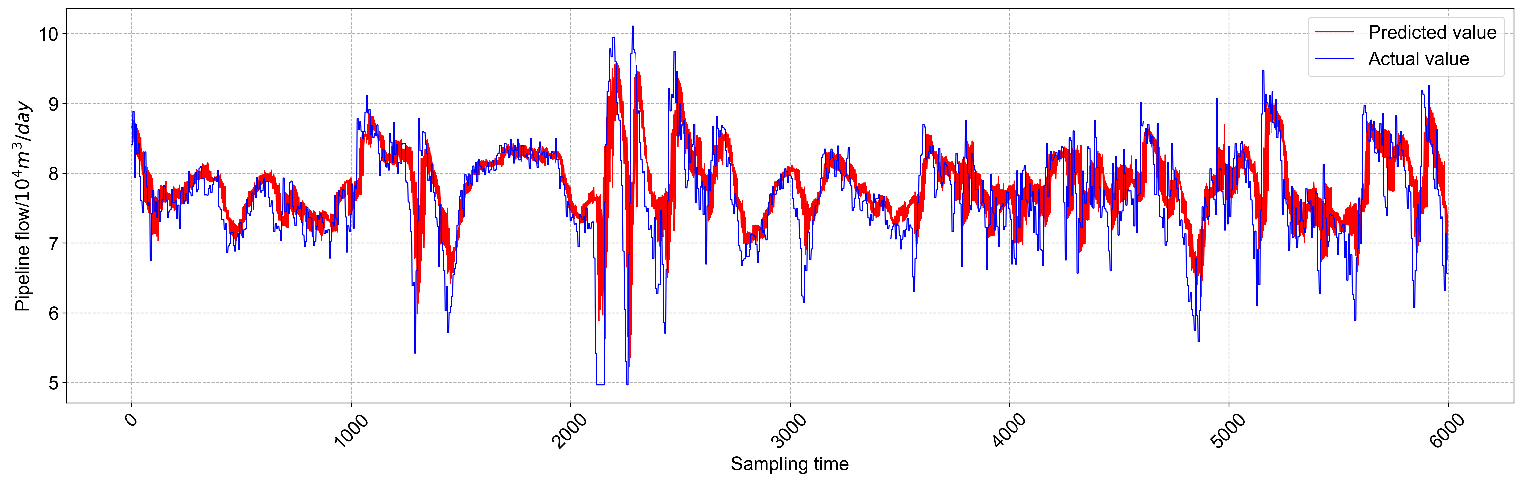
4.3. Comparison of Prediction Results

To verify the effectiveness of the proposed GSA-LSTM model, a comparison is made with the non-optimized LSTM model in

Table 4. Prediction results of the LSTM and GSA-LSTM method for the NG pipeline flow.

Method	RMSE	MAPE
LSTM	$0.5479$	$5.4722$
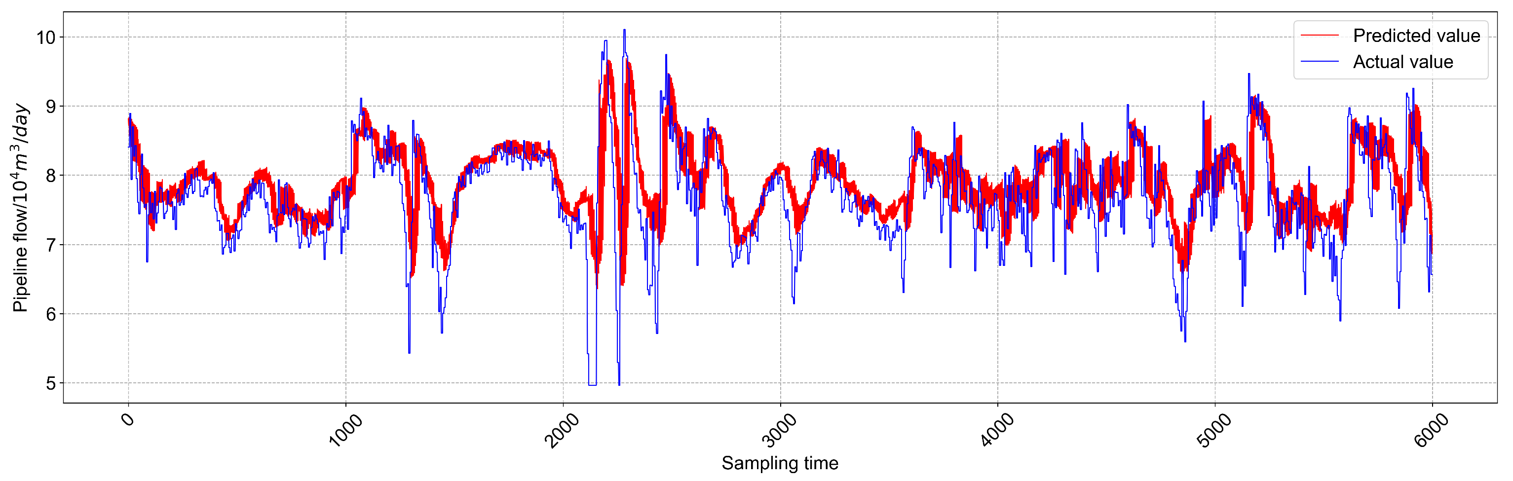
GSA-LSTM	$0.5017$	$4.8547$

. Note that five repeat experiments are conducted to average the prediction results to reduce the inherent randomness of neural network prediction. It is clearly seen that the RMSE and MAPE values of the GSA-LSTM are reduced by 8.43% and 11.28%, respectively, compared with the LSTM, which indicates that the proposed method obtains better prediction performance. Furthermore, Figure 8 and Figure 9 show the predicted trend plots of the NG pipeline flow obtained using the non-optimized LSTM and GSA-LSTM models, respectively. It is obvious that the proposed method can better capture the real-value curve than non-optimized LSTM.

Overall, the above experimental results confirm that the proposed GSA-LSTM method can effectively search for the optimal parameter combination for LSTM and captures the temporal features of the SCADA data, hence providing reliable predictions for the NG pipeline flow.

5. Conclusions

In this work, a prediction method for NG pipeline flow, namely GSA-LSTM, is proposed to solve the problem that traditional ML and statistical methods cannot extract temporal features from the SCADA data, which limits the accuracy of the prediction model. The proposed method first considers the correlation of the flow data of the SCADA at both ends of the pipeline, using the LSTM to learn the temporal information of the time series data at both ends of the pipeline. The past input and output of the pipeline system are used to predict the output at the next time step, effectively capturing the fluctuation trend of the original pipeline data. Then, the GSA optimization method is introduced to search for the optimal parameters for the LSTM, which solve the difficulty of manual-experience selection. Finally, a real-world NG pipeline system is carried out in the proposed method, and the experiment results demonstrate the superiority of the proposed method.

Thanks to the capability of the GSA-LSTM to analyze and predict the time series data with nonlinearity from the NG pipeline, future work will combine the prediction residual with the leak threshold to detect abnormal conditions. Since the healthy pipeline data train the model, the residual should be less than the leak threshold when the normal working condition data arrive. On the contrary, the model cannot adapt to the abnormal data when leakage occurs, and the residual will exceed the threshold range, thus realizing leakage detection.