Annual Electricity and Energy Consumption Forecasting for the UK Based on Back Propagation Neural Network, Multiple Linear Regression, and Least Square Support Vector Machine

Abstract

The long-term demand forecast for annual national electricity and energy consumption plays a vital role in future strategic planning, power system installation programming, energy investment planning, and next-generation unit construction. Three machine learning algorithms of BP-NN, MLR, and LS-SVM were chosen for training forecasting models, with the data on population, GDP, mean temperature, sunshine, rainfall, and frost days in 1993–2019 serving as the input variables. The total data were divided by 70% into the training set (1993–2011) and 30% into the test set (2012–2019), in chronological order. RMSE, MAPE, and MaxError were adopted as the performance criteria. The statistical results show that the gross population of the UK increases year by year from 1993 to 2020. The GDP generally increases before 2007 but has a decline, and then varies with a large amplitude afterward. The electricity and energy consumption of the UK generally increase from 1993 and reach a peak around 2005. Afterward, a decline occurs basically year by year until 2019. The simulation results reveal that all three models predict well on the training set but have some overestimation on the test set. The LS-SVM model has the best forecasting performance among the three models on the training set. The results show that it is feasible to use machine learning algorithms to predict the future electricity and energy consumption of a country based on past economic and livelihood data. In this way, economic decision-makers can rely on the predicted values to make a well-founded layout for future energy construction and investment to avoid waste or a shortage of resources.

1. Introduction

Energy is essential to humankind’s life and economic development. With the increase in population, as well as the socioeconomic and technological progress in the last few decades, energy consumption has significantly increased. The forecasting of energy demand plays a critical role in the electrical power industry and thermal energy supply. According to the forecast time range, demand forecasts can be roughly divided into three kinds [1], i.e., short-term forecasts, medium-term forecasts, and long-term forecasts. The long-term consumption forecast is defined as the forecast for 1–50 years. It is vital in future national strategic planning, energy investment planning, new generation unit construction, and electric power system installation planning.

One of the distinguishing characteristics of electricity is that it is difficult to store once generated. In addition, due to the internal complexity and irregularity of various interacting factors, such as gross domestic product (GDP), energy imports, energy exports, technological development, industrial production, population, and employment, it is hard to forecast energy consumption [2]. The gross population is one of the significant factors closely related to energy consumption. It is also popular to consider economic indicators such as GDP, employment, and inflation. With the increase in GDP per capita, people’s living standards are improving, and their way of life is increasingly dependent on appliances and equipment that consume energy. Therefore, a precise forecast of future electricity and energy consumption is greatly significant for reasonable future planning, new power generation investment, and the balance maintenance between energy supply and demand.

In the literature, many forecasting techniques are put forward to predict the consumption of electricity and thermal energy. These techniques can be divided into artificial neural networks (ANN), regression models, time series models, expert systems, fuzzy logic, grey predictions, support vector machines (SVM), and generic algorithms, and forecasting questions can be answered on an annual, monthly, weekly, daily, and hourly basis, as listed in Table 1. It cannot be said that every applied technique is fit for all prediction conditions. Energy consumption forecasting by machine learning techniques has been employed in many fields such as country primary energy and secondary energy, electricity markets based on renewable energy [3,4], smart grids [5,6,7], intelligent communities [8], office buildings [9], and CO₂ emissions [10]. In this work, the country energy demand prediction based on machine learning techniques will be mainly discussed, and the literature review is listed in Table 1.

The literature review shows that plenty of research has been carried out, aimed at energy demand forecasting for a country by predicting model input variables including GDP, import and export amounts, population, installed power capacity, yearly ambient temperature, yearly per resident electricity, the stock index, electricity price, natural gas price, inflation percentage, unemployment percentage, electricity demand per capita, CPI, and the increasing income rate. The yielded models are based on different types of machine learning techniques including MLR, ANN, SVM, LSTM, CNN, SVR, BPNN, GRU-ANN, the deep learning approach, grey prediction theory, ELM, and RNN. Meanwhile, some advanced algorithms have been applied in the training process of forecasting models to speed up the computing process or improve accuracy. It cannot be said that every technique used is appropriate for all the problems with prediction, and there is no optimal technique suitable for all prediction problems. For a specific problem, the actual situation must be considered to choose a predictive model. Nevertheless, it is summarized from the literature review that the models based on the ANN, MLR, and SVM techniques are frequently used to forecast annual national electricity and energy consumption, and the forecasting models based on these three techniques show better performance than other models under most conditions.

Generally speaking, electricity and energy consumption in developing countries increase year by year, so it is relatively easy to be forecasted in the previous literature. However, due to weak macroeconomic development, electricity and energy consumption in developed countries are not increasing year by year but varying rather irregularly. Therefore, the accuracy and feasibility of the forecast for developed countries are lower than that for developing countries. The above literature review reveals that few studies are aiming at annual electricity and energy forecasts for the old, developed countries in Europe. Thus, it is necessary to make a forecast for the UK.

In this work, three machine learning techniques—the backpropagation neural network (BP-NN), multiple linear regression (MLR), and least square support vector machine (LS-SVM)—are selected from numerous algorithms due to their extensive application and excellent performance in the previous literature practices. These three methods are employed to train models to predict the future annual electricity and thermal energy demand of the UK by 2020, based on the variables of demographical change, economic indicators, and climate data selected in 1993–2019, mainly from the website of GOV.UK [11]. Furthermore, some performance criteria are adopted to evaluate the performance of the three forecasting techniques, and the three methods are compared with each other to make the simulation results more convincing.

Table 1. Literature review.

References	Methods	Input Variables	Response Variables	Main Findings
Geem, Z. W. et al., 2009 [12]	ANN (momentum process, error backpropagation algorithm, feed-forward multilayer perceptron)	GDP, population, imports, exports	annual energy demand in South Korea	Energy demands reached a peak in specific years and then declined. The proposed model forecasted energy consumption greater than a linear regression model or an exponential model.
Ekonomou, L., 2010 [13]	artificial neural networks (with multilayer perceptron model)	GDP, annual per capita electricity consumption, installed capacity, yearly environment temperature	annual energy consumption in Greece	The produced ANN results show better accuracy than an SVM method and a linear regression method for the years 2005–2008.
Kandananond, K., 2011 [14]	multiple linear regression (MLR), ANN, ARIMA	population, GDP, income from the export of industrial products, stock index	annual electricity consumption in Thailand	The ANN model decreases the MAPE to 0.996%, while the MLR and ARIMA methods are 3.26% and 2.81%, respectively.
Azadeh, A. et al., 2013 [15]	ANN (multi-layer perceptron)	GDP, oil price, gas price, carbon monoxide, carbon dioxide, nitrogen oxide, lagged variable	monthly renewable energy consumption in Iran	The suggested method is helpful for locations without measuring equipment and has more advantages than conventional and fuzzy regression models.
Kialashaki, A., 2014 [16]	MLR, ANN	GDP, diesel fuel price, refiner price of propane, total energy consumption	annual energy demand in the American industry sector	The predictive result is consistent with the published forecast.
Kaytez, et al., 2015 [17]	neural networks, regression analysis, minimum blocks SVM	installed power capacity, GDP, total population, and subscribership data in 1970–2009	annual electricity consumption in Turkey	The proposed LS-SVM model shows accurate and rapid performance for forecasting.
Aydin, G. et al., 2016 [18]	ANN	population, GDP, imports, exports	annual energy consumption in the highest energy consumption countries	The correlation coefficients between actual energy demands and the ANN model predictions are higher than 90%.
Günay, M. E. et al., 2016 [19]	MLR, ANN	average summer and winter temperatures, population, GDP, inflation percentage, unemployment percentage	annual electricity demand in Turkey	Unemployment and average winter temperatures were negligible in determining the demand. The results are verified with high accuracy.
Berriel, R. F. et al., 2017 [20]	convolutional and deep fully connected neural networks	standardized average energy demand based on past 12 months	monthly electricity consumption	The proposed model can forecast with a relative error of 17.29% and an absolute error of 31.83 kWh.
Liu, B. et al., 2017 [21]	MLR, SVR, gated recurrent unit (GRU), ANN	GDP, population, imports, exports	annual primary energy consumption in China	The derived GRU model results indicate that China’s energy demand may change from 2954.04 Mtoe in 2015 to 5618.67 Mtoe in 2021.
Pino-Mejías, R., 2017 [22]	linear regression models, ANN	equipment load, air flow rate, infiltration rate, lighting load, occupant load, intensity of use, indoor design condition, thermal inertia	cooling and heating energy demands, other energy	In the case of energy demand and CO2 emissions, the linear regression models that provide better capability are those in which the predictor variables have been converted.
Zeng, Y. R. et al., 2017 [23]	BPNN model supported by adaptive differential evolution algorithms	GDP, population, imports, exports	annual electrical energy and total energy consumption	Compared with traditional anti-transmission neural network models and other common models, the ADE BPNN model can well forecast energy demand.
Li, M. et al., 2018 [24]	grey prediction theory optimized by SVM algorithm	coal, coal power demand in previous years	annual energy demand and CO2 emissions in Chinese Beijing–Tianjin–Hebei region	It is estimated that, by 2030, electricity and natural gas energy consumption will reduce to 45.0%, and the carbon emissions can be controlled to less than 96.9 million tons.
Mason, K. et al., 2018 [25]	neural network algorithm	historic and current values in the time series	monthly CO2 emissions, wind generation, and energy consumption in Ireland	The neural network is very competitive in predicting energy demand in Ireland, providing fast convergence, more robust and accurate forecasts.
Al-Musaylh et al., 2019 [26]	ANN	six climate variables (vapor pressure, solar radiation, evaporation, rainfall, max and min temperature) and 51 reanalysis variables	6 h and daily electricity consumption	The proposed neural network based on generic algorithm is more appropriate for short-term load predicting, and the proposed neural network predicts better for long term energy forecasting.
Hamzaçebi, C., 2019 [27]	ANN	Turkey’s previous monthly electricity consumption	Turkey’s monthly electricity consumption	The ANN model makes successful and high-precision predictions of Turkey’s monthly electricity demand from 2015 to 2018.
Laib, O. et al., 2019 [28]	Long-short-term memory recurrence neural network	temperature	daily and hourly natural gas consumption in Algeria	The results are compared with three methods: LSTM, MP neural network method, and seasonal time series of out-of-source variable models.
Zagrebina, S. et al., 2019 [29]	recurrent neural network	data of production calendars, meteorological factors (precipitation, clouds, wind speed, temperature, daylight length, etc.)	daily electricity consumption in Southern and Siberian Federal Districts in Russia	The recurrent neural network is constructed to produce more accurate prediction results.
AJ del Real. et al., 2020 [30]	a hybrid architecture consisting of an ANN and a sink neural network.	predicted weather data	monthly electricity demand of the French Grid	The solution gets the highest performance score among traditional ANN models and automatic decreasing integrated moving averages (ARIMA).

Table 1. Literature review.

References	Methods	Input Variables	Response Variables	Main Findings
Geem, Z. W. et al., 2009 [12]	ANN (momentum process, error backpropagation algorithm, feed-forward multilayer perceptron)	GDP, population, imports, exports	annual energy demand in South Korea	Energy demands reached a peak in specific years and then declined. The proposed model forecasted energy consumption greater than a linear regression model or an exponential model.
Ekonomou, L., 2010 [13]	artificial neural networks (with multilayer perceptron model)	GDP, annual per capita electricity consumption, installed capacity, yearly environment temperature	annual energy consumption in Greece	The produced ANN results show better accuracy than an SVM method and a linear regression method for the years 2005–2008.
Kandananond, K., 2011 [14]	multiple linear regression (MLR), ANN, ARIMA	population, GDP, income from the export of industrial products, stock index	annual electricity consumption in Thailand	The ANN model decreases the MAPE to 0.996%, while the MLR and ARIMA methods are 3.26% and 2.81%, respectively.
Azadeh, A. et al., 2013 [15]	ANN (multi-layer perceptron)	GDP, oil price, gas price, carbon monoxide, carbon dioxide, nitrogen oxide, lagged variable	monthly renewable energy consumption in Iran	The suggested method is helpful for locations without measuring equipment and has more advantages than conventional and fuzzy regression models.
Kialashaki, A., 2014 [16]	MLR, ANN	GDP, diesel fuel price, refiner price of propane, total energy consumption	annual energy demand in the American industry sector	The predictive result is consistent with the published forecast.
Kaytez, et al., 2015 [17]	neural networks, regression analysis, minimum blocks SVM	installed power capacity, GDP, total population, and subscribership data in 1970–2009	annual electricity consumption in Turkey	The proposed LS-SVM model shows accurate and rapid performance for forecasting.
Aydin, G. et al., 2016 [18]	ANN	population, GDP, imports, exports	annual energy consumption in the highest energy consumption countries	The correlation coefficients between actual energy demands and the ANN model predictions are higher than 90%.
Günay, M. E. et al., 2016 [19]	MLR, ANN	average summer and winter temperatures, population, GDP, inflation percentage, unemployment percentage	annual electricity demand in Turkey	Unemployment and average winter temperatures were negligible in determining the demand. The results are verified with high accuracy.
Berriel, R. F. et al., 2017 [20]	convolutional and deep fully connected neural networks	standardized average energy demand based on past 12 months	monthly electricity consumption	The proposed model can forecast with a relative error of 17.29% and an absolute error of 31.83 kWh.
Liu, B. et al., 2017 [21]	MLR, SVR, gated recurrent unit (GRU), ANN	GDP, population, imports, exports	annual primary energy consumption in China	The derived GRU model results indicate that China’s energy demand may change from 2954.04 Mtoe in 2015 to 5618.67 Mtoe in 2021.
Pino-Mejías, R., 2017 [22]	linear regression models, ANN	equipment load, air flow rate, infiltration rate, lighting load, occupant load, intensity of use, indoor design condition, thermal inertia	cooling and heating energy demands, other energy	In the case of energy demand and CO2 emissions, the linear regression models that provide better capability are those in which the predictor variables have been converted.
Zeng, Y. R. et al., 2017 [23]	BPNN model supported by adaptive differential evolution algorithms	GDP, population, imports, exports	annual electrical energy and total energy consumption	Compared with traditional anti-transmission neural network models and other common models, the ADE BPNN model can well forecast energy demand.
Li, M. et al., 2018 [24]	grey prediction theory optimized by SVM algorithm	coal, coal power demand in previous years	annual energy demand and CO2 emissions in Chinese Beijing–Tianjin–Hebei region	It is estimated that, by 2030, electricity and natural gas energy consumption will reduce to 45.0%, and the carbon emissions can be controlled to less than 96.9 million tons.
Mason, K. et al., 2018 [25]	neural network algorithm	historic and current values in the time series	monthly CO2 emissions, wind generation, and energy consumption in Ireland	The neural network is very competitive in predicting energy demand in Ireland, providing fast convergence, more robust and accurate forecasts.
Al-Musaylh et al., 2019 [26]	ANN	six climate variables (vapor pressure, solar radiation, evaporation, rainfall, max and min temperature) and 51 reanalysis variables	6 h and daily electricity consumption	The proposed neural network based on generic algorithm is more appropriate for short-term load predicting, and the proposed neural network predicts better for long term energy forecasting.
Hamzaçebi, C., 2019 [27]	ANN	Turkey’s previous monthly electricity consumption	Turkey’s monthly electricity consumption	The ANN model makes successful and high-precision predictions of Turkey’s monthly electricity demand from 2015 to 2018.
Laib, O. et al., 2019 [28]	Long-short-term memory recurrence neural network	temperature	daily and hourly natural gas consumption in Algeria	The results are compared with three methods: LSTM, MP neural network method, and seasonal time series of out-of-source variable models.
Zagrebina, S. et al., 2019 [29]	recurrent neural network	data of production calendars, meteorological factors (precipitation, clouds, wind speed, temperature, daylight length, etc.)	daily electricity consumption in Southern and Siberian Federal Districts in Russia	The recurrent neural network is constructed to produce more accurate prediction results.
AJ del Real. et al., 2020 [30]	a hybrid architecture consisting of an ANN and a sink neural network.	predicted weather data	monthly electricity demand of the French Grid	The solution gets the highest performance score among traditional ANN models and automatic decreasing integrated moving averages (ARIMA).

2. Methods

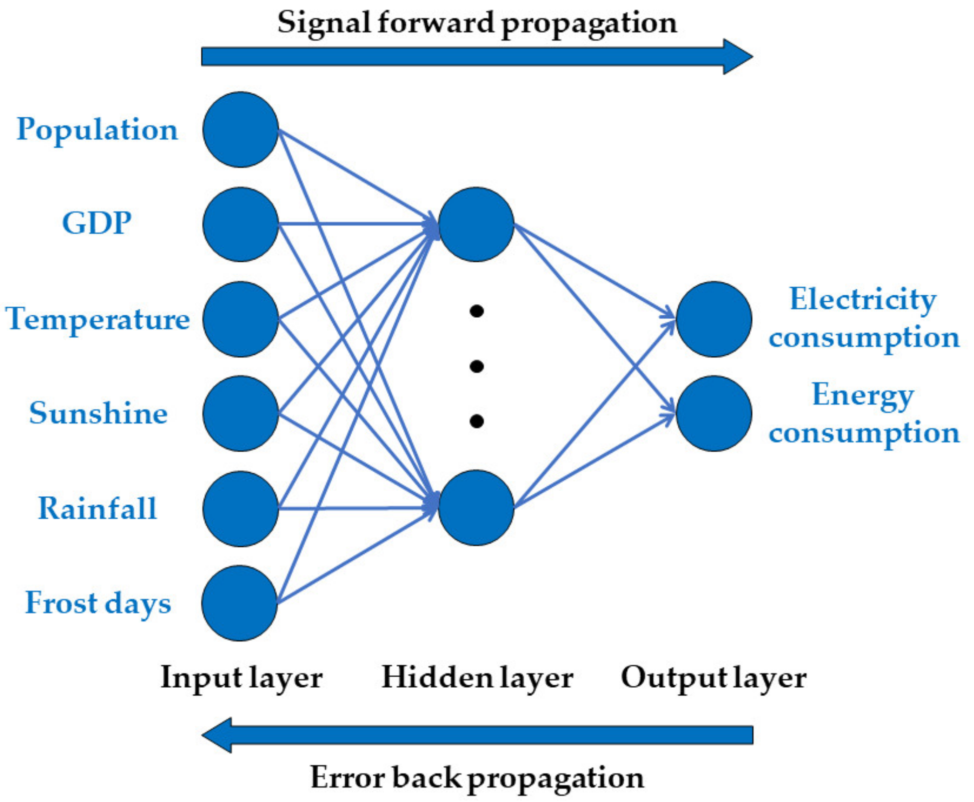
2.1. Back Propagation Neural Network

ANN is an intelligent algorithm that simulates the way a human’s brain analyzes and processes information. Hundreds of billions of neuronal cells are contained in the human brain, and every neuron is composed of a cell body that inputs and outputs information to assist the brain in its work. ANN has many artificial neurons connected to each other through nodes as processing units, and the processing units are also composed of units concerning input and output. By receiving different structures and forms of information, after processing by the interior weighting system, the neural network generates an output report from the presented information.

BP-NN is a widely used and successful neural network in the forecasting fields. BP-NN is a multi-layer feed to the neural network, and its main features are error propagation backward and signal propagation forward. It consists of an input layer, an output layer, and a few hidden layers. There are a certain number of nodes on each layer, and the number can be decided by the following empirical formula.

$${\displaystyle \sum _{i=0}^n{C}_{n_i}^i}>K$$

(1)

where n is the number of the input layer node; n_i is the number of the hidden layer node; and K is the sample number.

There are two single flows between the layers of BP-NN. The first is the forward propagation of the working signal from the input layer to the hidden layer and to the output layer. It is the function of input data and the weight matrix. The second is the reverse propagation of the error signal from the output layer to the hidden layer, and eventually to the input layer. The error signal is the difference between the true output and expected output, and the error $E_p$ can be calculated using the equation as follows.

$$E_p=\frac{1}{2}\ast {{\displaystyle \sum \left(t_{pi}-o_{pi}\right)}}^2$$

(2)

where $t_{pi}$ represents the expected output, and $o_{pi}$ denotes the true output.

In the BP-NN, the node connection between the layers is full, but there is no connection on the single layer. The upper layer nodes connect to the lower layer nodes by the weight matrix, and the ordinary transfer function is the sigmoid function.

$$f\left(x\right)=\frac{1}{1+e^{-x}}$$

(3)

During the process of working signal and error propagation, the weight matrix is constantly adjusted. In the end, when the actual output is consistent with the expected output, the back propagation neural network can be used for forecasting directly.

Figure 1 shows the BP-NN model used in this work, which contains the input layer, output layer, and one hidden layer. In the input layer, the population, GDP, mean temperature, sunshine, rainfall, and days of air frost are employed as the input parameters. Meanwhile, the electricity consumption and inland consumption of primary fuels and the equivalents for energy use are set as the output parameters that are intended to be forecasted in this work.

2.2. Multiple Linear Regression

MLR is a multivariate promotion of simple linear regression. The input variable x changes from a single feature to a vector containing k features. Each eigenvector is multiplied by a coefficient and added to a final offset, as displayed in the following equation.

$$y=b_0+b_1\ast x_1+b_2\ast x_2+\mathrm{\dots }+b_k\ast x_k$$

(4)

where $y$ is the dependent variable; $x_1$ to $x_k$ are the independent variables; $b_1$ to $b_k$ are the regression coefficients of $x_1$ to $x_k$; and $b_0$ is the constant error term. In this work, to construct the multiple linear regression model, the independent variables of $x_1$ to $x_k$ were the population, GDP, mean temperature, sunshine hours, rainfall, and frost days, while the dependent variable $y$ was the annual electricity and energy consumption of the UK. The regression coefficient is obtained by minimizing the sum of squares of the deviation between the actual dependent value and the predicted dependent value and adjusting the error term $b_0$.

2.3. Least Square Support Vector Machine

The SVM model originates from statistical theory and is widely used for nonlinear regression problems. However, the computing process of the SVM is complex, due to the long and computationally difficult quadratic programing in the e-insensitive loss function. To address this issue, the LS-SVM was introduced by Suykens et al. [31]. The LS-SVM uses the least square loss function to construct the optimization problem based on equality constraints, and the least square loss function requires only the solution of a linear equation series. For the training data set $\left(x_i,y_i\right), i=1,\cdots ,N$ (N is the number of training data), and $x_i\in R^d$ and $y_i\in R$ are the input and output variables, respectively. The regression function can be formulated using a nonlinear function $\phi \left(x\right)$ to map the input space to a feature space.

$$y\left(x\right)={\omega }^T\phi \left(x\right)+b$$

(5)

where $\omega$ and $b$ are the parameters to be calculated.

On the basis of the rule of structural risk minimization [31], the regression problem of LS-SVM can be converted into a constrained optimization problem.

$$\{\begin{array}{l}\underset{\omega ,\xi }{\min }\frac{1}{2}{\omega }^T\omega +\frac{\gamma }{2}{\displaystyle \sum _{i=1}^N{\xi }_{\mathrm{i}}^2, \gamma >0}\\ \mathrm{subjective} \mathrm{to} y_i={\omega }^T\phi \left(x_i\right)+b+{\xi }_i, i=1,\cdots ,N\end{array}$$

(6)

where ${\xi }_i$ is the error, and $\gamma$ represents the penalty factor. A corresponding Lagrange function is constructed to simplify the computation by transforming the problem into its dual space.

$$L\left(\omega ,b,\xi ,\beta \right)=\frac{1}{2}{\omega }^T\omega +\frac{\gamma }{2}{\displaystyle \sum _{i=1}^N{\xi }_{\mathrm{i}}^2-{\displaystyle \sum _{i=1}^N{\beta }_i}}\left[{\omega }^T\phi \left(x_i\right)+b+{\xi }_i-y_i\right]$$

(7)

where ${\beta }_i$ is the Lagrange multiplier. Based on the Karush–Kuhn–Tucker (KKT) condition, the conditions for optimality are

$$\{\begin{array}{l}\frac{\partial L}{\partial \omega }=0 \to \omega ={\displaystyle \sum _{i=1}^N{\beta }_i\phi \left(x_i\right)}\\ \frac{\partial L}{\partial b}=0 \to {\displaystyle \sum _{i=1}^N{\beta }_i=0}\\ \frac{\partial L}{\partial {\xi }_i}=0 \to {\beta }_i=\gamma {\xi }_i\\ \frac{\partial L}{\partial {\beta }_i}=0 \to {\omega }^T\phi \left(x_i\right)+b+{\xi }_i-y_i=0\end{array}$$

(8)

By eliminating the variables $\omega$ and ${\xi }_i$, the LS-SVM regression model can be redefined as

$$(\begin{array}{l}0\\ e_n\end{array}\begin{array}{l} e_n^T\\ \mathsf{\Omega }+{\gamma }^{-1}{e}_n\end{array})\left(\begin{array}{l}b\\ \beta \end{array}\right)=\left(\begin{array}{l}0\\ y\end{array}\right)$$

(9)

where $e_n={\left(1,\cdots ,1\right)}^T$ represents the unit matrix; $\beta ={\left({\beta }_1,\cdots ,{\beta }_N\right)}^T$ represents the Lagrange multiplier matrix; $y={\left(y_1,\cdots ,y_N\right)}^T$ is the output variable matrix. $\mathsf{\Omega }$ is a symmetric matrix of the kernel function, where ${\mathsf{\Omega }}_{ij}$ is calculated as

$${\mathsf{\Omega }}_{ij}=K\left(x_i,x_j\right)=\phi {\left(x_i\right)}^T\phi \left(x_j\right), i=1,\cdots ,N$$

(10)

where $K\left(x_i,x_j\right)$ represents the kernel function. The $\beta$ and $b$ could be obtained by solving Equation (9). Then the regression equation of the LS-SVM can be written as

$$y\left(x\right)={\displaystyle \sum _{i=1}^N{\beta }_{i}K\left(x_i,x_j\right)}+b$$

(11)

Mercer’s condition [32] must be satisfied by applicable Kernel functions, which can be typically either linear, polynomial, or radial basis function kernels. The radial basis function kernel is employed in this study as shown below

$$K\left(x_i,x_j\right)=\exp \left(-{\Vert x_i-x_j\Vert }^2/{\delta }^2\right)$$

(12)

where $\delta$ is the bandwidth of the radial basis function kernel.

3. Application

3.1. Data

Population, GDP, mean temperature, sunshine, rainfall, and days of air frost are employed as the input variables, and electricity consumption and the inland consumption of primary fuels and the equivalents for energy use are employed as the output variables. In energy consumption, primary fuels refer to coal, petroleum, and natural gas. The equivalents for energy use refer to net electricity imports, wind and hydroelectricity, nuclear electricity, and bioenergy and waste. (For convenience, the term “energy consumption” is used to replace inland consumption of primary fuels and the equivalents for energy use in some paragraphs.) The statistical data on population [33] and GDP [34] are from the World Bank; the data on weather are from the Met Office [35]; and the data on electricity and energy consumption are from the UK government’s official website [36]. Although the population and GDP data have a wide period, the weather data is limited to 1993–2020. Therefore, this relatively short period is chosen for the study subjects, as listed in

Table 2. Original data of input and output variables.

Year	Population (Millions)	GDP (USD)	Mean Temperature (°C)	Sunshine (Hours)	Rainfall (mm)	Air Frost (Days)	Electricity Consumption (TWh)	Energy Consumption (Million Tons)
1993	57.7	1.06 × 1012	8.33	1211	1149.7	56	295.75	220.73
1994	57.9	1.14 × 1012	8.89	1358.8	1216.5	48.1	292.83	217.47
1995	58	1.35 × 1012	9.17	1579.5	1050.3	65.5	303.92	218.39
1996	58.2	1.42 × 1012	8.18	1389.7	935.2	77	319.78	229.99
1997	58.3	1.56 × 1012	9.41	1420	1048.7	49.4	321.07	226.81
1998	58.5	1.65 × 1012	9.16	1258	1298.5	46.8	325.35	230.74
1999	58.7	1.69 × 1012	9.37	1406.7	1271.8	43.8	332.05	231.33
2000	58.9	1.66 × 1012	9.1	1358.2	1372.5	43.2	340.30	234.81
2001	59.1	1.64 × 1012	8.8	1406.7	1049.4	70.7	342.50	236.85
2002	59.4	1.78 × 1012	9.44	1297.2	1280.4	36.4	344.11	229.60
2003	59.6	2.06 × 1012	9.47	1586.3	900.1	60.2	346.62	231.87
2004	60	2.42 × 1012	9.44	1355.5	1208.9	46.6	347.71	233.63
2005	60.4	2.54 × 1012	9.42	1381.9	1079.6	53.6	357.20	236.29
2006	60.8	2.72 × 1012	9.7	1472.3	1173.2	51.7	353.86	233.07
2007	61.3	3.11 × 1012	9.56	1436.1	1195.7	39.2	351.45	227.49
2008	61.8	2.94 × 1012	9.02	1375.2	1293.2	57.9	349.53	225.67
2009	62.3	2.43 × 1012	9.14	1465.7	1208.1	56.9	329.42	211.68
2010	62.8	2.49 × 1012	7.94	1444.5	945.4	93.4	337.51	219.31
2011	63.3	2.67 × 1012	9.61	1398	1162.6	41.3	325.92	203.59
2012	63.7	2.72 × 1012	8.74	1332.1	1329.7	54.9	325.48	207.80
2013	64.1	2.80 × 1012	8.74	1410.9	1084	71.1	324.38	206.26
2014	64.6	3.09 × 1012	9.88	1416.6	1292.8	31.7	310.80	193.60
2015	65.1	2.96 × 1012	9.18	1445	1265.3	43.9	311.42	195.05
2016	65.6	2.72 × 1012	9.29	1417.4	1096.7	54	311.30	192.46
2017	66	2.70 × 1012	9.53	1369.3	1118.5	48.3	306.79	190.62
2018	66.4	2.90 × 1012	9.45	1560.1	1053.6	54	307.37	189.52
2019	66.8	2.88 × 1012	9.39	1454.4	1232.3	48.1	302.50	184.48
2020	67.2	2.76 × 1012	9.62	1497.4	1336.3	37.7

. All the 1993–2019 data are allocated according to the ratio of 70% as the training set (1993–2011) and 30% as the test set (2012–2019), in chronological order, and the output data for 2020 is predicted, based on the models established in the following section.

It is evident from Figure 2 that the gross population of the UK increases year by year from 1993 to 2020. In addition, the population growth rate significantly speeds up after 2006. The gross population reaches 67.2 million in 2020, which is a new historical peak. The GDP of the UK generally increases before 2007 but has a decline after 2007 and varies later, with a large amplitude, which indicates weak and unhealthy economic development. The climate data, including mean temperature, sunshine, rainfall, and air frost, vary little year by year and generally maintain a stable level from 1993 to 2020.

Figure 3 illustrates that electricity consumption in the UK increases from 1993 and reaches a peak in 2005. However, the electricity consumption starts to decline year by year from 2005 to 2019. The energy consumption varies with a similar tendency to that of the electricity consumption. The energy consumption generally augments from 1993 to 2005 but basically decreases from 1993 to 2019. It is speculated that the variations in electricity and energy consumption are closely related to the change in GDP due to the same inflection point. In addition, though the population increases and the GDP generally remains unchanged after 2005, the electricity and energy consumption decrease year by year, which demonstrates that the economic development is less and less dependent on electricity and energy consumption. A healthier and greener economic operation is generated and developed in the old, developed country of the UK.

3.2. Performance Criterions

Some common parameters are selected to measure the merits of the three models, including root mean square error (RMSE), mean absolute percentage error (MAPE), and maximum error (MaxError). The above-mentioned performance criteria are defined by the following equations [17,27].

$$\mathrm{RMSE}=\sqrt{\frac{{\displaystyle {\sum }_{k=1}^N{\left(y_f-y_r\right)}^2}}{N}}$$

(13)

$$\mathrm{MAPE}(\%)=100\times \frac{{\displaystyle {\sum }_{k=1}^N\left|\frac{y_f-y_r}{y_r}\right|}}{N}$$

(14)

$$\mathrm{MaxError}=\max \left|y_f-y_r\right|$$

(15)

where $y_r$, $y_f$, and $N$ represent the original data on electricity and energy consumption, the forecasted value, and the number of years, respectively.

4. Results and Discussion

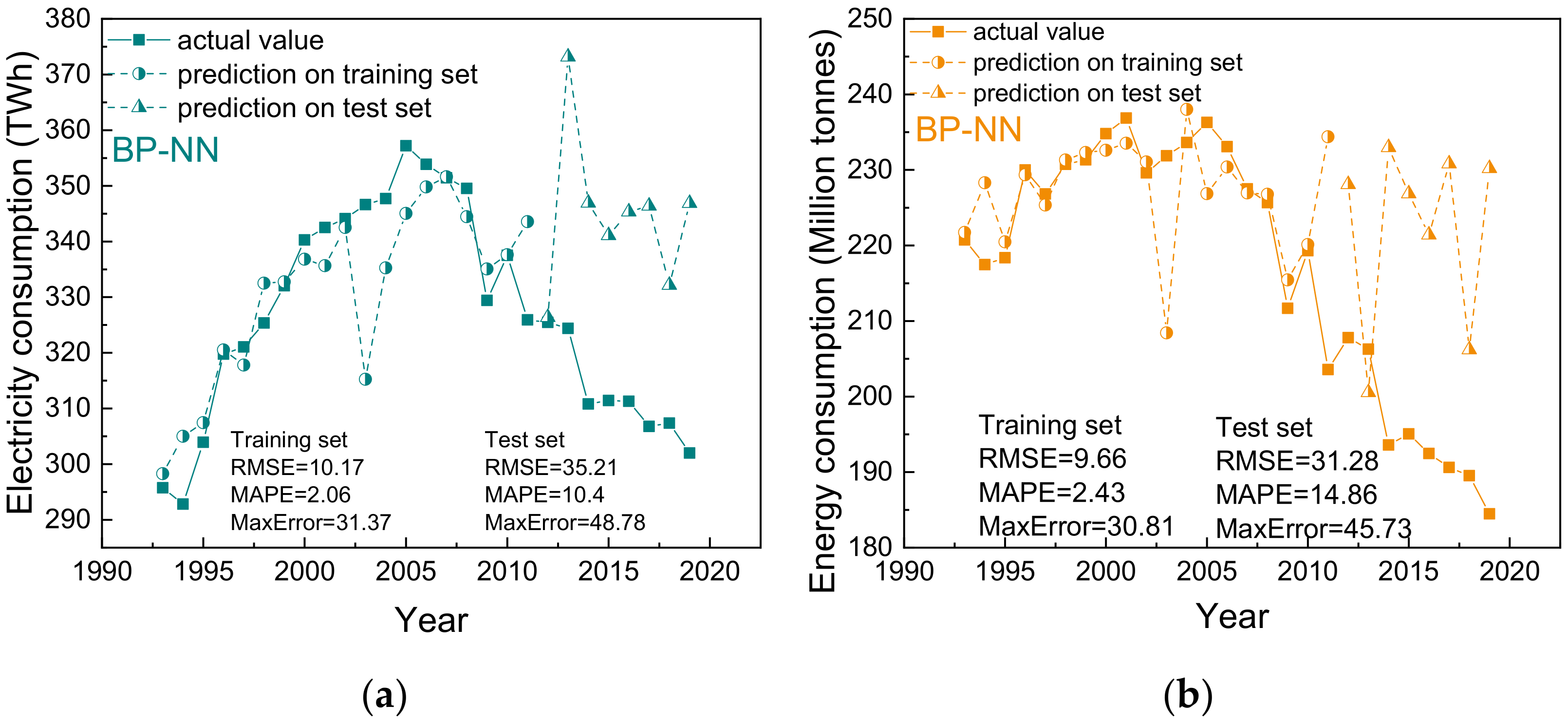
4.1. Results of BP-NN Model

Many parameters impact the performance of the BP-NN model such as the number of hidden layers, the number of training iterations, the learning rate, and the minimum number of confirmed failures. Considering that the amount of data is relatively small and more hidden layers may cause counterproductive effects, the number of hidden layers is finally decided to be one. The hidden layer has 20 parameters, 1000 training iterations, a learning rate of 0.01, and a minimum number of 200 confirmation failures, as shown in Figure 4.

It is obvious in Figure 5 that the forecasting performance on most points of the training set is very good, but it generally has an overestimation on the test set, whether for electricity consumption or energy consumption. The reason for this will be explained in Section 4.4. In addition, it seems that the weather data are negligible in determining the annual electricity and energy demand.

4.2. Results of MLR Model

Figure 6 shows that the predictive tendency of the MLR model is similar to that of the BP-NN model, but the forecasting deviation in the training set is larger. The forecasting deviation of the MLR model in the test set is close to the BP-NN model, while the fluctuation range of predictive values reduces. MLR is an ideal model and very simple in structure, which might lead to a large difference between the MLR and the actual situation. Thus, MLR has the poorest forecasting performance among the three models.

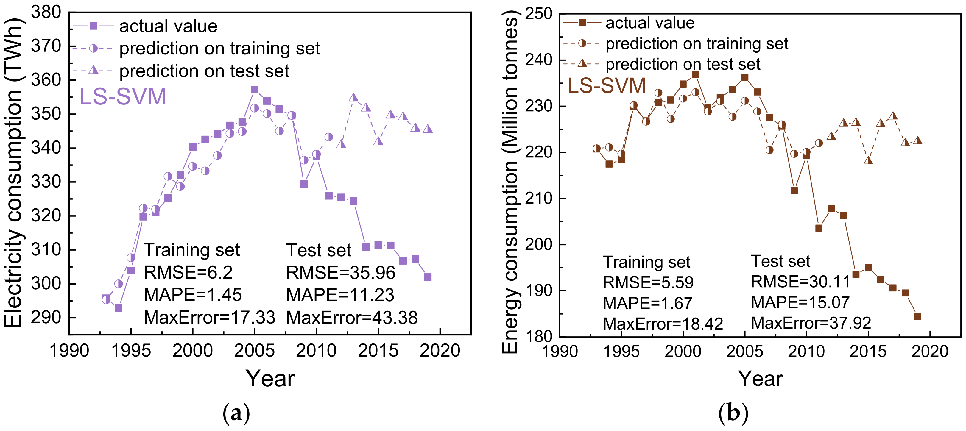
4.3. Results of LS-SVM Model

Figure 7 illustrates that the forecasting performance of the LS-SVM model on most points of the training set is very good, but it generally has an overestimation in the test set, whether for electricity consumption or energy consumption. The predictive tendency of the LS-SVM model is similar to that of the BP-NN model and the MLR model, but the forecasting deviation of the LS-SVM model in the training set is the least among the three models. In addition, all three models overestimate the test set, and the deviations and performance criteria are similar to each other.

4.4. Comparison of Three Models

It is summarized from the above content that the LS-SVM model has the best forecasting performance among the three models in the training set, no matter what kind of criteria is used. All three models also predict well in the training set but overestimate in the test set, and the reason could be explained as:

(1)

The original data on electricity and energy consumption do not vary consistently. The consumption data first increases and then decreases. For the training set, the increasing trend points account for the vast majority, and the declining trend points account for little, which might contribute to the overestimation on the test set.

(2)

GDP is strongly correlated with electricity and energy consumption before 2007, but the correlation weakens, speculated as the fact that the GDP varies with fluctuations but generally remains unchanged, while the electricity and energy consumption decrease year by year after 2007. Though the economic development becomes healthy and green, the forecasting for electricity and energy consumption gets tough when GDP is used as one of the most important input variables for the model. Therefore, more correlated economic indicators should be introduced into the input variables.

(3)

The total data is extracted from 1993 to 2019, and this relatively small amount of data could not train a perfect model to forecast annual national electricity and energy consumption.

Furthermore, to enhance the forecasting performance of the trained model, several improvement measures should be taken in the future as follows:

(1)

The data in the training set should have a similar variation tendency to the total dataset.

(2)

More economic indicators correlated with energy consumption should be introduced into the input variables for the forecasting model.

(3)

More data should be collected, and the starting year of the dataset extended to an earlier date.

4.5. Prediction of Future Data

The model input variables (population, GDP, mean temperature, sunshine, rainfall, and days of air frost) for 2020 have been collected and listed in Table 2. Hence, the electricity and energy consumption values for 2020 could be forecasted by the three trained models in this work, and the predictive values are listed in

Table 3. Predictive values in 2020.

2020	Actual Value	BP-NN	MLR	LS-SVM
Electricity consumption (TWh)	287.47	344.68	319.34	321.25
Energy consumption (Million tons)	162.51	228.34	203.34	206.7

. When the LS-SVM model is employed, it is forecasted that the electricity consumption in 2020 is 321.25 TWh, and the energy consumption in 2020 is 206.7 million tons.

Table 3 shows that both electricity and energy consumption in 2020 are slightly less than the forecast data in this paper. This is consistent with the trend that the predicted value in the test set is a little larger. In addition, affected by the COVID-19 pandemic, the reduction in electricity and energy consumption compared to previous years is also a major reason for the overestimation.

This means that the only six input variables used in this study are not enough to predict the country’s annual electricity and energy consumption, due to the COVID-19 pandemic after 2020. The key parameters related to the COVID-19 pandemic and other necessary parameters must be added into the input variables of the machine learning model for better forecasting, which might be conducted in our future work.

5. Conclusions

In this work, the annual electricity and energy consumption for the UK was intended to be forecasted by machine learning techniques. BP-NN, MLR, and LS-SVM were employed to train forecasting models, with population data, GDP, mean temperature, sunshine, rainfall, and days of air frost in 1993–2019 serving as the input variables. All the data are allocated according to the ratio of 70% as the training set (1993–2011) and 30% as the test set (2012–2019), in chronological order. To appraise the predictive model’s performance and make inter-comparisons, the RMSE, MAPE, and MaxError were adopted as the performance criteria. Several main conclusions are listed as follows.

(1)

The weather data are negligible in determining the national annual electricity and energy consumption.

(2)

Electricity and energy consumption have a strong correlation with GDP before 2007, but the correlation weakens after 2007, indicating that a greener economic pattern is generated and developed.

(3)

The LS-SVM model shows better forecasting performance than the BP-NN and MLR models in the training set.

The study in this paper shows that it is feasible to use machine learning algorithms to predict the future electricity and energy consumption values of a country based on past economic and livelihood data. In this way, economic decision-makers can rely on the predicted values to make a well-founded layout for future national strategic planning, energy investment planning, construction of new generating units, power system installation planning, etc., to avoid waste or a shortage of resources.

In addition, other than electricity and energy consumption predictions, the objective of trained models could be extended to the forecasting of CO₂ emissions, the smart grid, and intelligent community electricity consumption in the future.

References

1. Koprinska, I.; Rana, M.; Agelidis, V.G. Correlation and instance based feature selection for electricity load forecasting. Knowl. Based Syst. 2015, 82, 29–40. [Google Scholar] [CrossRef]
2. Tang, L.; Wang, S.; He, K.; Wang, S. A novel mode-characteristic-based decomposition ensemble model for nuclear energy consumption forecasting. Ann. Oper. Res. 2015, 234, 111–132. [Google Scholar] [CrossRef]
3. Acaroğlu, H.; García Márquez, F.P. Comprehensive review on electricity market price and load forecasting based on wind en-ergy. Energies 2021, 14, 7473. [Google Scholar] [CrossRef]
4. Dubey, A.K.; Kumar, A.; Ramirez, I.S.; Marquez, F.P.G. A Review of Intelligent Systems for the Prediction of Wind Energy Using Machine Learning. In International Conference on Management Science and Engineering Management; Springer: Cham, Switzerland, 2022; pp. 476–491. [Google Scholar]
5. Hafeez, G.; Javaid, N.; Ullah, S.; Iqbal, Z.; Khan, M.; Rehman, A.U. Short Term Load Forecasting Based on Deep Learning for Smart Grid Applications. In International Conference on Innovative Mobile and Internet Services in Ubiquitous Computing; Springer: Cham, Switzerland, 2018; pp. 276–288. [Google Scholar]
6. Hafeez, G.; Javaid, N.; Riaz, M.; Ali, A.; Umar, K.; Iqbal, Z. Day Ahead Electric Load Forecasting by an Intelligent Hybrid Model Based on Deep Learning for Smart Grid. In Conference on Complex, Intelligent, and Software Intensive Systems; Springer: Cham, Switzerland, 2019; pp. 36–49. [Google Scholar]
7. Hafeez, G. Electrical Energy Consumption Forecasting for Efficient Energy Management in Smart Grid. Ph.D. Thesis, COMSATS University of Islamabad, Islamabad, Pakistan, 2021. [Google Scholar]
8. Pirbazari, A.M.; Sharma, E.; Chakravorty, A.; Elmenreich, W.; Rong, C. An ensemble approach for multi-step ahead energy forecasting of household communities. IEEE Access 2021, 9, 36218–36240. [Google Scholar] [CrossRef]
9. Runge, J.; Zmeureanu, R. A review of deep learning techniques for forecasting energy use in buildings. Energies 2021, 14, 608. [Google Scholar] [CrossRef]
10. Hosseini, S.M.; Saifoddin, A.; Shirmohammadi, R.; Aslani, A. Forecasting of CO2 emissions in Iran based on time series and regression analysis. Energy Rep. 2019, 5, 619–631. [Google Scholar] [CrossRef]
11. UK Government. “Postcode Level Domestic Gas and Electricity Consumption: About the Data” Datasheet, Mar. 2017. Available online: https://www.gov.uk/government/publications/postcode-level-domestic-gas-and-electricity-consumption-about-the-data (accessed on 30 July 2021).
12. Geem, Z.W.; Roper, W.E. Energy demand estimation of South Korea using artificial neural network. Energy Policy 2009, 37, 4049–4054. [Google Scholar] [CrossRef]
13. Ekonomou, L. Greek long-term energy consumption prediction using artificial neural networks. Energy 2010, 35, 512–517. [Google Scholar] [CrossRef] [Green Version]
14. Kandananond, K. Forecasting Electricity Demand in Thailand with an Artificial Neural Network Approach. Energies 2011, 4, 1246. [Google Scholar] [CrossRef] [Green Version]
15. Azadeh, A.; Babazadeh, R.; Asadzadeh, S. Optimum estimation and forecasting of renewable energy consumption by artificial neural networks. Renew. Sustain. Energy Rev. 2013, 27, 605–612. [Google Scholar] [CrossRef]
16. Kialashaki, A.; Reisel, J.R. Development and validation of artificial neural network models of the energy demand in the industrial sector of the United States. Energy 2014, 76, 749–760. [Google Scholar] [CrossRef]
17. Kaytez, F.; Taplamacioglu, M.C.; Cam, E.; Hardalac, F. Forecasting electricity consumption: A comparison of regression analysis, neural networks and least squares support vector machines. Int. J. Electr. Power Energy Syst. 2015, 67, 431–438. [Google Scholar] [CrossRef]
18. Aydin, G.; Jang, H.; Topal, E. Energy consumption modeling using artificial neural networks: The case of the world’s highest consumers. Energy Sources Part B Econ. Plan. Policy 2016, 11, 212–219. [Google Scholar] [CrossRef]
19. Günay, M.E. Forecasting annual gross electricity demand by artificial neural networks using predicted values of socio-economic indicators and climatic conditions: Case of Turkey. Energy Policy 2016, 90, 92–101. [Google Scholar] [CrossRef]
20. Berriel, R.F.; Lopes, A.T.; Rodrigues, A.; Varejao, F.M.; Oliveira-Santos, T. Monthly energy consumption forecast: A deep learning approach. In Proceedings of the 2017 International Joint Conference on Neural Networks (IJCNN), Anchorage, AK, USA, 14–19 May 2017; pp. 4283–4290. [Google Scholar]
21. Liu, B.; Fu, C.; Bielefield, A.; Liu, Y.Q. Forecasting of Chinese Primary Energy Consumption in 2021 with GRU Artificial Neural Network. Energies 2017, 10, 1453. [Google Scholar] [CrossRef]
22. Pino-Mejías, R.; Pérez-Fargallo, A.; Rubio-Bellido, C.; Pulido-Arcas, J.A. Comparison of linear regression and artificial neural networks models to predict heating and cooling energy demand, energy consumption and CO2 emissions. Energy 2017, 118, 24–36. [Google Scholar] [CrossRef]
23. Zeng, Y.R.; Zeng, Y.; Choi, B.; Wang, L. Multifactor-influenced energy consumption forecasting using enhanced back-propagation neural network. Energy 2017, 127, 381–396. [Google Scholar] [CrossRef]
24. Li, M.; Wang, W.; De, G.; Ji, X.; Tan, Z. Forecasting carbon emissions related to energy consumption in Beijing-Tianjin-Hebei region based on grey prediction theory and extreme learning machine optimized by support vector machine algorithm. Energies 2018, 11, 2475. [Google Scholar] [CrossRef] [Green Version]
25. Mason, K.; Duggan, J.; Howley, E. Forecasting energy demand, wind generation and carbon dioxide emissions in Ireland using evolutionary neural networks. Energy 2018, 155, 705–720. [Google Scholar] [CrossRef]
26. Al-Musaylh, M.S.; Deo, R.C.; Adamowski, J.F.; Li, Y. Short-term electricity demand forecasting using machine learning methods enriched with ground-based climate and ECMWF Reanalysis atmospheric predictors in southeast Queensland, Australia. Renew. Sustain. Energy Rev. 2019, 113, 109293. [Google Scholar] [CrossRef]
27. Hamzaçebi, C.; Es, H.A.; Çakmak, R. Forecasting of Turkey’s monthly electricity demand by seasonal artificial neural network. Neural Comput. Appl. 2019, 31, 2217–2231. [Google Scholar] [CrossRef]
28. Laib, O.; Khadir, M.T.; Mihaylova, L. Toward efficient energy systems based on natural gas consumption prediction with LSTM Recurrent Neural Networks. Energy 2019, 177, 530–542. [Google Scholar] [CrossRef]
29. Zagrebina, S.; Mokhov, V.; Tsimbol, V. Electrical Energy Consumption Prediction is based on the Recurrent Neural Network. Procedia Comput. Sci. 2019, 150, 340–346. [Google Scholar] [CrossRef]
30. Del Real, A.J.; Dorado, F.; Durán, J. Energy Demand Forecasting Using Deep Learning: Applications for the French Grid. Energies 2020, 13, 2242. [Google Scholar] [CrossRef]
31. Suykens, J.A.; Vandewalle, J.; De Moor, B. Optimal control by least squares support vector machines. Neural Netw. 2001, 14, 23–35. [Google Scholar] [CrossRef]
32. Mercer, J. Xvi. functions of positive and negative type, and their connection the theory of integral equations. Philos. Trans. R. Soc. London. Ser. A Contain. Pap. A Math. Phys. Character 1909, 209, 415–446. [Google Scholar]
33. World Bank. “Population, Total—United Kingdom” Datasheet. Available online: https://data.worldbank.org.cn/indicator/SP.POP.TOTL?locations=GB (accessed on 30 July 2021).
34. World Bank. “GDP (Current DOLLARS)—United Kingdom” Datasheet. Available online: https://data.worldbank.org.cn/indicator/NY.GDP.MKTP.CD?end=2020&locations=GB&start=1960&view=chart (accessed on 30 July 2021).
35. United Kingdom Meteorological Office. “Synoptic and Climate Data in All Weather Stations” Datasheet. Available online: https://www.metoffice.gov.uk/weather/learn-about/how-forecasts-are-made/observations/weather-stations (accessed on 30 July 2021).
36. Department for Business, Energy & Industrial Strategy. “Historical Electricity Data: 1920 to 2020” Datasheet. Available online: https://www.gov.uk/government/statistical-data-sets/historical-electricity-data (accessed on 29 July 2021).
Figure 1. BP-NN model used in this work.
Processes 11 00044 g001
Figure 2. Variations of original data for input variables in 1993–2020. ((a) population; (b) GDP; (c) mean temperature; (d) sunshine; (e) rainfall; (f) air frost).
Processes 11 00044 g002
Figure 3. Variations of original data for output variables in 1993–2019. ((a) electricity consumption; (b) energy consumption).
Processes 11 00044 g003
Figure 4. Parameter setting of BP-NN model.
Processes 11 00044 g004
Figure 5. Results of BP-NN model. ((a) electricity consumption; (b) energy consumption).
Processes 11 00044 g005
Figure 6. Results of MLR model. ((a) electricity consumption; (b) energy consumption).
Processes 11 00044 g006
Figure 7. Results of LS-SVM model. ((a) electricity consumption; (b) energy consumption).
Processes 11 00044 g007