Article

Optimal Manufacturer Recycling Strategy under EPR Regulations

College of Management, Zhejiang University of Technology, Hangzhou 310023, China
*
Author to whom correspondence should be addressed.
Processes 2023, 11(1), 166; https://doi.org/10.3390/pr11010166
Submission received: 23 November 2022 / Revised: 23 December 2022 / Accepted: 26 December 2022 / Published: 5 January 2023
(This article belongs to the Special Issue Green Manufacturing and Sustainable Supply Chain Management)

Abstract

:
Under extended producer responsibility (EPR) regulations, trade-in programs allow manufacturers to play a vital role in recycling. Simultaneously, third-party recyclers (TPRs) can use their recycling network to compensate for manufacturers having only a single recycling channel, which increases the competition between them. To study whether companies should authorize TPRs, we constructed and analyzed a Stackelberg game model with trade-in programs under EPR regulations by focusing on three different closed-loop supply chain (CLSC) structures and differentiating consumer categories. The analytical results showed that when the government does not act as the decision maker, the optimal product selling price of the manufacturer does not change under each strategy. Otherwise, the manufacturer’s decision is affected by the cost structure and amount of subsidy, as well as funds determined by the government under the optimal environmental benefit. Furthermore, when the residual value coefficient of the used products is high, manufacturers authorize TPRs to recycle used products.

1. Introduction

With the rapid iteration of products, the amount of waste electrical and electronic equipment (WEEE) is rapidly increasing. According to statistics, the world produced 53.6 million tons of WEEE in 2019, an increase of nearly 21% in five years, of which only 17% was recycled [1]. The landfilling and incineration of a large amount of waste have seriously harmed the environment [2]. Therefore, many countries and regions have introduced relevant policies to deal with the waste disposal problem, especially recycling legislation based on extended producer responsibility (EPR); for example, the WEEE Directive in the European Union, the Japanese PC Recycling System, and the Beverage Bottle Recycling Act in the USA [3].
With the gradual strengthening of EPR regulations, original equipment manufacturers (OEMs) are finding it increasingly difficult to collect used products due to single recycling channels and incomplete recycling facilities [4]. For example, the WEEE Directive issued by the EU in 2005 requires member states to recycle WEEE accounting for at least 45% of the new product sales, and the target was raised to 85% in 2019 [5]. Unlike an OEM’s direct recycling channels, consumers can more conveniently complete recovery through third-party recycling channels [6]. For example, recycling platforms such as Ecoatm.com, Aihuishou, and Zhuanzhuan provide consumers with door-to-door recycling services so they may easily recycle used products [7]. Therefore, to increase recycling efficiency, manufacturers often choose to authorize a third-party recycler (TPR) to perform recycling [8].
Although the involvement of TPRs can help manufacturers fulfill EPR regulations, they often form a competitive relationship with manufacturers. In reality, to increase sales and prevent the loss of customers, manufacturers such as Apple, Huawei, Ford, Canon, and IBM often adopt a trade-in strategy through which customers can receive a price discount by returning their used products when purchasing a new one [9,10]. As such, a cannibalization effect exists between the TPRs and OEMs, and whether to authorize the TPRs has become a dilemma for OEMs [11]. As such, we addressed the following questions in this study aiming to help OEMs that may face similar challenges:
(1) Is it advisable for an OEM to authorize a TPR?
(2) How should an OEM adjust its strategies under the different intensities of the EPR regulation?
(3) How does government involvement impact on the OEM’s strategic choices?
To address the above questions, we divided our analyses into four parts:
(1) Not authorizing a TPR under exogenous funds and subsidies;
(2) Not authorizing a TPR under endogenous funds and subsidies;
(3) Authorizing a TPR under exogenous funds and subsidies;
(4) Authorizing a TPR under endogenous funds and subsidies.
According to the theoretical analysis, we determined the optimal pricing and the trade-in price discount, as well as the circumstances under which the OEM should choose to authorize a TPR. Our three main findings were:
(1) The OEM should be dedicated to retaining original consumers by enhancing its reputation, contributing to improvements in economic and environmental performance.
(2) Under the EPR regulations, an OEM should authorize a TPR when the residual value coefficient of the waste products is significant.
(3) When the government is involved in the closed-loop supply chain (CLSC), gaining profits is harder for the OEM through a trade-in program because the OEM has to provide more funds to the government.
The remainder of this paper is organized as follows. Section 2 illustrates our contributions through a literature review. Section 3 describes the model and outlines assumptions. Section 4 provides a detailed analysis based on the exogenous and endogenous aspects of government subsidies and funds. Section 5 outlines our numerical simulation. Section 6 draws the study conclusions.

2. Literature Review

Our study is related to three streams of literature: EPR regulations in CLSCs, the competition between OEMs and TPRs, and trade-ins.
The first stream of research relates to our study regards EPR regulations. Spicer et al. [12] discussed three methods to implement EPR regulations. Ozdemir et al. [13] studied the impact of manufacturer recycling decisions and product redesign under EPR. Esenduran et al. [14] analyzed the recycling competition between OEMs of electrical and electronic products and TPRs under EPR, and the changes in their strategies under different circumstances. Chen et al. [15] analyzed the effect of the reward and punishment mechanism in a green supply chain, especially its effect on the recovery rate of waste products. Chang et al. [16] considered the EPR system as a joint tax-subsidy mechanism in the production and recycling system. However, these researchers did not introduce cooperative benefits produced by TPRs under the EPR regulations. In this study, we considered the coopetition effect produced by TPRs and thoroughly analyzed the impact of EPR regulation on manufacturers’ strategic choices on whether to authorize TPRs.
Second, our study also relates to research on CLSCs including TPRs. Yan et al. [17] demonstrated that corporate social responsibility (CSR) can influence manufacturers’ willingness to cooperate with retailers or TPRs and cooperation strategy choices. Xing et al. [18] examined the impact of two risk-averse competing recyclers on the manufacturer’s low-carbon production. Zhang et al. [19] established a game model of the competition between legal and illegal recyclers with government involvement. Huang et al. [20] and Hong et al. [21] regarded the recovery cost and quantity as the recycling rate functions to investigate decisions and profits in CLSCs, where the TPR acted as a recycler. Chu et al. [22] studied the coordination problem between TPRs and multiple manufacturers, which outperformed individual retailer- and manufacturer-managed modes. Khan et al. [8] used an evolutionary game model to identify the economic principle behind original vehicle manufacturers when deciding whether to authorize TPRs. Our study is different from theirs in the following way. In our study, the government encouraged CLSCs toward sustainable directions by levying funds and providing subsidies, thus impacting coopetition between OEM and TPR.
The final stream of literature related to our study is related to trade-ins. According to Ray et al. [23], there exist optimal trade-in and pricing strategies of durable goods manufacturers. Xiao et al. [10] determined the most suitable channel form for implementing a trade-in strategy and found that when the consumer acceptance degree of the direct online channel changes, the optimal channel form accordingly changes. Li et al. [24] examined OEM optimal pricing, trade-in, and remanufacturing decisions when a secondary market cannibalization exists. Agrawal et al. [25] suggested that OEMs can choose alternative methods, including trade-in programs and offering remanufactured products, to compete with third-party remanufacturers. Hu et al. [26] demonstrated that consumer category and trade-in duration significantly impact the optimal strategy of a firm. These researchers all regarded trade-ins as merely a marketing tool for business, whereas we introduced EPR regulations through which the government can intervene in a trade-in program by levying funds from the firm and providing subsidies to original consumers.
This study contributes to the existing literature as follows. To the best of our knowledge, only some researchers have comprehensively considered the following three elements: TPR, EPR regulations, and trade-in programs. We fill this gap by investigating the economic principles that govern OEM behavior toward whether to authorize a TPR in an EPR environment while considering a trade-in program. In addition, the topic of trade-in programs has received increasingly extensive attention in academia. However, most investigators conducted their study with a relatively simple illustration of consumers’ utility functions. Original consumers’ perceptions may substantially impact new consumers’ purchasing behaviors, and we introduced this factor in our study to facilitate the formulation of EPR regulations and the implementation of recycling strategies.
This study provides insights for OEMs when formulating strategic decisions and governments when designing and implementing EPR regulations. In summary, we compare our study with related studies in Table 1.

3. Problem Description and Basic Assumptions

Under EPR regulations, the manufacturer provides a certain price discount to the original consumer who returns used products to buy new products through trade-in. The government, manufacturer, and third-party recycler are all independent decision makers, among which the government is the decision pioneer, and the manufacturer and third-party recycler are decision followers. The third-party recycler is also the decision follower of the manufacturer. For ease of understanding, the parameters and variables use in this study are shown in Table 2.
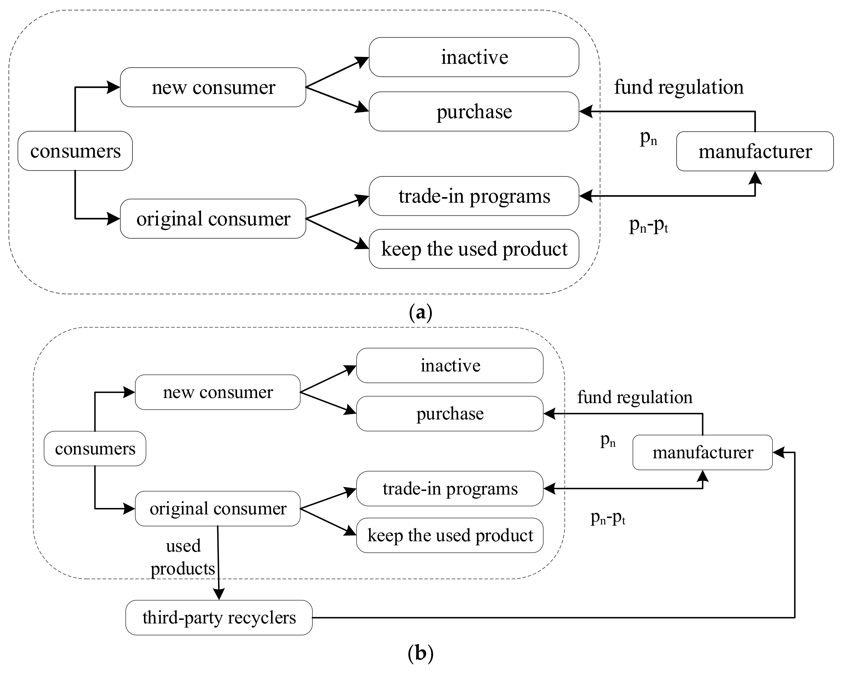
We considered the trade-in program as a marketing strategy of the manufacturer and as a recycling strategy to consider its participation in the recycling of used products under EPR regulations. In the market, a third-party recycler recycles various used products on a cash basis. We explored the optimal manufacturer decision and its influencing factors when the government outlines criteria for treatment funds and subsidies for used and end-of-life products. The manufacturer has two choices: 1. Not authorizing a third-party recycler to recycle used products, namely Model N, as shown in Figure 1a; 2. Authorizing third-party recyclers to recycle used products, namely, Models A and AC, as shown in Figure 1b. In Model A, the manufacturer does not compete with the third-party recycler; that is, for the manufacturer, whether the third-party recycler runs a recycling program does not affect the number of original consumers participating in trade-in programs. In Model A, no competitive relationship exists between the manufacturer and third-party recycler; that is, for the manufacturer, whether the third-party recycler runs a recycling program does not affect the number of original consumers participating in the trade-in program. In Model AC, the manufacturer competes with third-party recyclers. For some of the original consumers, participating in the recycling program conducted by third-party recyclers and participating in the trade-in program have the same effect. The two consumer groups overlap; that is, some of the original consumers who participated in the trade-in program choose to participate in the recycling program conducted by third-party recyclers. The third-party recycling activities are those in which the third-party recycler first collects the used product from the original consumer and then the manufacturer buys back the used product from the third-party recycler. The recycled used product can be used to produce remanufactured products, and the demand function we constructed in this study is similar to that of Hong et al. [27], assuming that the new product is of the same quality and price as the remanufactured product. We assumed that the new product produced by the manufacturer is of the same quality and price as the product remanufactured by the manufacturer. The manufacturer, which refers to a legitimate company with production and sales capacity and recycling and dismantling functions, is directly involved in the treatment and implementation of the standardized management of used products. The manufacturer and third-party recycler are certified by environmental protection authorities.
To facilitate and highlight the study, for both of these models, we made the following key assumptions and statements:
(1) We assumed that the production capacity of the manufacturer is large enough to meet the market demand, and the market demand is the product output [28,29].
(2) We assumed that the market size is 1, in which the proportion of original consumers (with used products) is α ( 0 α 1 ), and the rest are potential consumers, namely new consumers, with a proportion of 1 α .
(3) We assumed that the quality of the new product is the same as that of the remanufactured product; then, the unit cost of new products is c n , and the unit cost of the remanufactured products is c r . As the raw materials and energy consumption of r-manufactured products in the production process are often lower than those of new products [30], then the costs of new products and remanufactured products require 0 < c r < c n < 1 .
(4) To show economic value, p u < p t + s must be satisfied to prevent original consumers from participating in trade-in programs, and the discounted price of the used product plus the government subsidy should be higher than the recycling price of the third-party recycler.
(5) The willingness of new consumers to pay for new products is θ and follows a uniform distribution U 0 , 1 . In contrast to new consumers considering repurchase, the willingness to pay of the original consumer holding the used product is affected by the value surplus of the currently held products and the use experience and evaluation of the previous product [29].
a. Consider the existence of value surplus of used products. Assume that the residual value coefficient of used products is δ u , and the range is δ u 0 , 1 . If only the residual value coefficient of used products is considered, then the willingness of original consumer to pay is θ δ u θ .
b. Through the comprehensive use of the product, the original consumers form a comprehensive evaluation of the enterprise’s products, which is generally divided into people’s comprehensive use feelings and evaluation of the internal and external characteristics of the product, such as performance, quality, convenience, post-purchase conflict, emotional evaluation, brand awareness, etc. For the sake of argument and highlighting the contributions of our study, the above influence attributes are again combined into one influence coefficient [29]; i.e., the original consumer’s perceived value coefficient of the branded product β , and the value domain is β 0 , + , where the consumption intention to repurchase decreases. β > 1 indicates that the original consumer is satisfied with the experience of the branded product and feels that it is good value for money, and so the consumption intention to repurchase increases. Therefore, the original consumer’s willingness to pay is β θ δ u θ , again considering the original consumer’s feelings of use and evaluation.
(6) We assumed that when the manufacturer sells a unit product, the government collects a fund amount f , the government gives the original consumer a trade-in subsidy s , and the environmental benefit of formalized environmental treatment units for used products is e .
We referred to the study of Cao et al. [30] to construct a product demand function from consumer utility. Based on the above assumptions and the data in Table 2, we analyzed the product utility and demands of the new and original consumers under the two models as follows.
Assume that the manufacturer chooses not to authorize the third party to recycle its used products, which is Model N. We assume that in this market, the market size is 1, the share of original consumers is α , and the share of new consumers is 1 α . The utility that a new consumer can obtain from the product is U N = θ p n . If U N > 0 , the new consumer buys the product produced by the manufacturer. Therefore, under Model N, the demand of new consumers can be expressed as:
q N N = 1 α p n 1 d θ = 1 α 1 p n .  
Similarly, an original consumer under Model N can derive utility U O = β θ p n + p t δ u θ s from the trade-in program; when U O > 0 , this original consumer participates in the trade-in program conducted by the manufacturer. Therefore, the demand of trade-in program under Model N can be expressed as:
q O N = α p n p t s β δ u 1 d θ = α 1 p n p t s β δ u .
If the manufacturer chooses to authorize the third-party recycler to recover the used product, the original consumer obtains the product utility U O = β θ p n + p t δ u θ s . The original consumer receives utility U T = p u δ u θ for participating in recycling programs conducted by third-party recyclers. When U O > max U T , 0 , that original consumer participates in a trade-in program conducted by the manufacturer; when U T > max U O , 0 , the original consumer participates in the recycling program conducted by the third-party recycler.
If U T θ 2 = 0 > U O θ 2 , the original consumer obtains the same utility by participating in the manufacturer’s trade-in program as by keeping the used product. If U T θ 2 = 0 > U O θ 2 , the original consumer obtains the same utility by participating in a recycling activity conducted by a third-party recycler as by keeping the used product; if U O θ 3 = U T θ 3 = 0 , buying a new product is no different than participating in a third-party recycling program for the original consumer: θ 1 = p n p t s β δ u ; θ 2 = p u δ u ; θ 3 = p n p t s + p u β .
If θ 1 > θ 2 , no competition exists between the trade-in program conducted by the manufacturer and the recycling program conducted by the third-party recycler in which the original consumer participates. As shown in Figure 2, we define such a case as Model A. Thus, in such a case, the purchase demand of the original consumer for products can be expressed as:
q O A = α p n p t s β δ u 1 d θ = α 1 p n p t s β δ u .
The demand for recycling programs conducted by (participating) third-party recyclers is:
q T A = α p u δ u 1 d θ = α p u δ u .
If θ 1 < θ 2 , a competitive relationship exists between the trade-in program conducted by the manufacturer and the recycling program conducted by the third-party recycler in which the original consumer participates. As shown in Figure 3, we define such a situation as Model AC. In this case, the original consumer’s used products are all recycled. Thus, the demand for the product purchased by the original consumer can be expressed as:
q O A C = α p n p t s β δ u 1 d θ = α 1 p n p t s + p u β .
The demand for recycling programs conducted by (participating) third-party recyclers is:
q T A C = α 0 p n p t s + p u β d θ = α p n p t s + p u β .

4. Supply Chain Model in Three Different Cases

4.1. Model N

4.1.1. Not Considering Government as Decision Maker

Under Model N, the manufacturer chooses not to authorize the third party to recycle its used products. The manufacturer sets product prices p n N and trade-in discounts p t N to maximize profits.
The profit function of the manufacturer under Model N, based on the demand function of the new and original consumers, is:
m a x p n , p t Π M N = q N N p n N c n f + q O N p n N c r p t N f s . t .   q N N > 0 & q T N > 0 .
By solving the first-order derivative optimal value, the optimal product price and optimal trade-in price discount set by the manufacturer are obtained as follows (see Appendix A for the solving process):
p n N = 1 + c n + f 2
p t N = 1 β + Δ s + δ u 2
Proposition 1.
The equilibrium optimal solution and optimal profit of the trade-in closed-loop supply chain model without the participation of third-party recyclers are shown in Table 3.
Corollary 1.
For Model N, the monotonicity of q N N , q O N   a n d   Π M N with respect to β , δ u , c n , c r , s , and f is shown inTable 4.
See Appendix B for the proof.
According to Proposition 1, we drew the following main conclusions: (1) When the manufacturer decides the optimal product price p n N and the optimal trade-in price discount p t N , it does not need to consider the proportion of original consumers in the market, and separately optimizes the product selling price for the two types of consumers to achieve profit maximization. The main reason is that the manufacturer can easily distinguish the two types of consumers, and the manufacturer can directly implement differentiated pricing for these two types. (2) The demands of new q N N and original q O N consumers increase with the decrease in the production costs of the unit new product c n and the unit remanufactured product c r , respectively, so that the manufacturer’s profit Π M N increases. This means that the manufacturer can improve the production technology and reduce the unit production cost, thereby increasing market demand and profit, indicating that technological innovation is crucial to the manufacturer. (3) The manufacturer’s profit is positively correlated with the product brand perception coefficient β . The manufacturer cannot perform a one-shot deal and needs to maintain long-term customer relationships and perform well in after-sales service to obtain a positive effect. When the original consumer’s tendency to continue to consume is low (i.e., β δ u is small, as δ u is determined by the nature of the product; namely, β is small), the manufacturer further increases the price discount on the trade-in to urge the original consumer to buy its product again. When the original consumer has a larger unit tendency to continue to consume, the manufacturer reduces the trade-in price discount. That is, when the original consumers have low purchase desire, the manufacturer needs to pay more for the used products to offset the cost when implementing the trade-in program, so as to attract the original consumers, which is similar to the situation in real life.
Corollary 1 shows that the optimal profit of manufacturers within the scope of the feasible region has a monotone decreasing function with c n , f , and δ u , and a monotone increasing function with s and β . This suggests that the lower the manufacturer’s production cost, the lower the perception coefficient of used products, the smaller the used product treatment fund collected by the government, and the larger the price subsidy and brand perception coefficient provided by the government, the higher the manufacturer profit.

4.1.2. Considering Government as Decision Maker

Based on the discussion above and the literature, the government’s environmental benefit function can be expressed as [23]:
Π G N G = q O N G e s N G + f N G + q N N G f N G  
Substitute the above q N N _ and q O N _ into Equations (5)–(9). By solving the first-order derivative optimal value, the optimal government subsidy and the optimal levy fund amount are obtained at this time as follows (the solving process is detailed in Appendix C):
s N G = 1 β + δ u Δ + e 2  
f N G = 1 c n 2  
s N G is the government subsidy provided to the original consumer for the trade-in, so s N G 0 ,   which needs to obey β + Δ e δ u < 1 . Using the backward induction method, we can determine the optimal decision of the manufacturer to implement the trade-in program under fund regulation, as shown in Table 5.
Proposition 2.
Under fund regulation, the equilibrium optimal solution and optimal profit of the trade-in closed-loop supply chain model with the government as the decision maker and without the participation of third-party recyclers are shown in Table 5.
Proposition 2 shows that: (1) Regardless of whether the government subsidizes the original consumers who participate in the trade-in program, the amount of funds for each unit of used product treatment levied by the government on the manufacturer does not change and does not affect the manufacturer’s pricing of the product. (2) Under the regulation of the fund, the optimal amount of the used product treatment fund levied by the government on the manufacturer is f N G = 1 c n 2 , which decreases with increases in the manufacturer’s cost of producing new products. (3) When the government provides a certain subsidy, s N G = 1 β + δ u Δ + e 2 , the subsidy decreases as the original consumer perception coefficient of the product brand, and product cost savings decrease. At the same time, the subsidy increases with the increase in the environmental benefits of recycling and processing units of used products and the perceived coefficient of used products. This indicates that government subsidies help manufacturers to increase the recycling rate of used products, the value of reusing, and the recycling capacity.

4.2. Model A

4.2.1. Not Considering Government as a Decision Maker

Under Model A, the manufacturer is responsible for product production and sales, as well as implementing the trade-in programs, whereas the third-party recycler is responsible for recycling used products. A Stackelberg game exists between the manufacturer and third-party recycler, and no competition exists between the trade-in programs of manufacturers and the recycling activities of third parties. That is, the manufacturer first sets the sales price of the product p n A , the discount on the trade-in price p t A , and the transfer price b A . Accordingly, the third-party recycler sets the recycling price of the used product p u A . The optimization problem of the third-party recycler is as follows:
m a x p u Π T A = q T A b A p u A
For q T A , as shown in Equation (4), the optimal solution of the third-party recycler optimization problem can be obtained p u A p n A , p t A , b A . The manufacturer’s optimization problem is:
m a x p n , p t Π M A = q N A p n A c n f + q O A p n A c r p t A f + Δ b q T A s . t .   0 < q O A + q α   &   q N A q T A
This problem is a typical Stackelberg game. Solving Equations (13) and (14) by backward induction can obtain the following (refer to Appendix D for the solution procedure):
Proposition 3.
Under fund regulation, the equilibrium optimal solution and optimal profit of the trade-in closed-loop supply chain model with the government not acting as the decision maker and with the participation of third-party recyclers and no competition are shown in Table 6.
Proposition 3 states that: (1) If the product is in the growth period, the optimal price of the product under Model A p n A and the optimal discount of the trade-in price p t A are the same as those under Model N. Correspondingly, the demands from new consumers q N A and original consumers q O A do not change, which indicates that when the residual value coefficient of used products is large, the third-party recycling program does not affect the trade-in program of the manufacturer. (2) p u A = Δ 4 , meaning that the recovery price is only related to cost savings and not to other factors; that is, although the residual value coefficient of the used product is high, it affects neither the recovery price of its recycled used product nor the manufacturer’s trade-in program. (3). Π M A Π M N = α Δ 2 8 δ u > 0 ; compared with Model N, the manufacturer can also obtain additional income from the recycling activities conducted by the third-party recycler under Model A.
Corollary 2.
For Model A, the monotonicity of q N A , q O A , q T A , Π M A , and Π T A with respect to β , δ u , c n , c r , s , and f is shown inTable 7  (see Appendix E for the proof).
Corollary 2 shows that if the amount of used product treatment funds collected by the government increases, the demand of new consumers and original consumers decreases, and the manufacturer’s profit also decreases, which means that the government should properly consider the amount of used product treatment funds to collect.

4.2.2. Government as Decision Maker

The government’s environmental benefit function can be expressed as follows:
m a x s A G , f A G Π G A G = q O A G + q T A G e s A G + f A G + q N A G f A G .
By substituting q N A and q O A into Equation (15), the optimal government subsidy and the optimal collection fund amount can be obtained as follows through the first-order derivative optimal value-solving steps (see Appendix F for the solving process):
s A G = Δ 4 δ u β Δ 4 + e + 1 β + δ u 2 ,
f A G = 1 c n 2 .
s A G is a government subsidy provided to original consumers for trade-ins, so s A G 0 ; that is, it requires 1 + Δ 2 δ u β δ u e + Δ < 1 . The backward induction method can be used to determine the optimal decision of the manufacturer to implement the trade-in program under fund regulation, as shown in Table 8. The solution process is shown in Appendix F.
Proposition 4.
Under the fund regulation, the equilibrium optimal solution and optimal profit of the trade-in closed-loop supply chain model with the government acting as the decision maker and with the participation of third-party recyclers and no competition are shown in Table 8.
Proposition 4 shows that: (1) When the government does not subsidize the original consumers involved in the trade-in program, the factors influencing the manufacturer’s optimal selling price and optimal discount on the trade-in program do not change, indicating that the recycling activities of third-party recyclers do not affect the manufacturer’s trade-in programs. (2) When the government subsidizes the original consumers involved in the trade-in program, the discount in the trade-in price provided by the manufacturer to the original consumer changes; the variable is Δ p t A G = Δ 8 δ u β δ u . This means that the manufacturer increases the price discount for the trade-in program without changing the selling price of the product, meaning that the price discount received for the original consumer increases after authorizing a third-party recycler to recycle the used product. (3) The government’s unit subsidy for the original consumer in the trade-in program s A G = Δ 4 δ u β Δ 4 + e + 1 β + δ u 2 changes; the change amount is Δ s A G = Δ 4 δ u β δ u . That is, compared with the absence of a third-party recycler, the government reduces the subsidy provided to the original consumer who participates in the trade-in program. For the government, with the participation of third-party recyclers, the quantity of recycled used products can be guaranteed. (4) For the original consumer, under Model NG, the price to purchase the product is p n A G p t A G s A G = 3 β δ u + c r e 4 . Under Model AG, the price to purchase the product is p n A G p t A G s A G = 3 β δ u + c r e 4 + Δ 8 δ u β δ u . Therefore, the price paid by the original consumer to purchase the same product increases, and the consumer surplus decreases.

4.3. Model AC

Under Model AC, the game between manufacturers and third-party recyclers is a Stackelberg game, and competition exists between manufacturers’ trade-in programs and the recycling activities of third-parties. That is, the manufacturer first sets the sales price of the product p n A C , trade-in price discount p t A C , and transfer price b A C . Based on this, the third-party recycler sets the price of recycling the used product p u A C . According to the reverse-order method, the optimization problem of the third-party recycler is:
m a x p u A C Π T A C = q T A C b A C p u A C .
q T A C , as shown in Equation (6), is used to obtain the optimal solution to the third-party recycler optimization problem p u A C p n A C , p t A C , b A C . The manufacturer’s optimization problem is:
m a x p n A C , p t A C Π M A C = q N A C p n A C c n f + q O A C p n A C c r p t A C f + Δ b A C q T A C s . t .   0 < q O A C + q T A C α & q N A C q T A C .
Similarly, the equilibrium optimal solution of the two-player game in Model AC can be obtained by backward induction (see Appendix G for the solution procedure). Substitute optimal equilibrium solutions into Equations (18) and (19) to obtain the optimal profit for the manufacturer and the third-party recycler.
Proposition 5.
Under fund regulation, the equilibrium optimal solution and optimal profit of the trade-in closed-loop supply chain model with the government not acting as the decision maker and the participation of third-party recyclers and the presence of competition are shown in Table 9.
Corollary 3.
For Model AC, the monotonicity of q N A C , q O A C , q T A C , Π M A C , and Π T A C with respect to β , δ u , c n , c r , s , and f is shown in Table 10. See Appendix Hfor the proof.
Proposition 5 and Corollary 3 show that: (1) When the government does not act as the decision maker, the optimal product price p n A C and demand of new consumers q N A C under Model AC are equal to the optimal product price and demand of new consumers under Model N, which means that the recycling activities of third parties do not affect the manufacturer’s product price. (2) When s f c n 2 Δ β + δ u , the trade-in price discount under Model AC p t A C is larger than that under Model N p t N , which means that when the unit subsidy of the trade-in program minus the collected used product treatment fund is less than the critical value, the manufacturer needs to increase the trade-in discount to cope with the recycling competition from the third-party recyclers. (3) The demand of original consumers also accordingly changes. The number of original consumers participating in the trade-in programs increases. Similarly, when s f c n 2 Δ β + δ u , the demand for the trade-in program under Model AC q O A C is larger than that under Model N q O N .

4.3.1. Government as Decision Maker

The government’s environmental benefit function can be expressed as:
m a x s A C G , f A C G Π G A C G = α e s A C G + f A C G + q N A C f A C G .
By substituting the above q N A C into Equation (20) and solving the first-order derivative optimal value, the optimal government subsidy and optimal levy fund amount can be obtained, respectively, as follows (see Appendix I for the solving process):
s A C G = 0 ,
f A C G = 1 c n 2 + α 1 α .
Substituting s A C G and f A C G into Equations (18) and (19), the optimal solution can be obtained as shown in Table 11.
Proposition 6.
Under fund regulation, the equilibrium optimal solution and optimal profit of the closed-loop supply chain model with the participation and competition of the government as the decision maker and the third-party recycler are shown in Table 11.
Proposition 6 shows the following: (1) The optimal trade-in price discount p t A C G formulated by the manufacturer is unrelated to cost saving Δ A C G . Under Model AC, the original consumers no longer own the used products, and all the used products are recycled and manufactured into remanufactured products, so the cost of remanufactured products does not affect the price discount formulated by the manufacturer. (2) The optimal product price p n A C G rises because the government levies higher treatment funds on manufacturers for used products. Hence, the manufacturer can realistically and logically pass this on to the consumer, with the consumer and the manufacturer each bearing 50% of the cost. In a sense, the fund regulation system works, forcing the manufacturer to take responsibility for the disposal of used products. (3) The pricing of the manufacturer’s products is different from the expression under Model NG, indicating that the development of the trade-in program changes the product’s selling price and consumers’ original perception of payment. With the increase in the proportion of original consumers, the product selling price increases. In this case, the durability of the used products is low, and the brand perception coefficient is large, which shows that the original consumers have high stickiness and higher repurchase desire. Accordingly, as a rational entity, the manufacturer raises the price, reduces consumer surplus, and increases its own profit.

5. Numerical Simulation Analysis

Combined with the abovementioned conditions and conclusions, to deeply understand the impact of the market environment on the manufacturer’s profit, we selected different parameters in the feasible region and analyzed the results through numerical simulation using the software named PyCharm.

5.1. Impact of Fund Regulation on Manufacturer Profit

We set the residual value coefficient of used products δ u   to   0.1 ; unit production cost of new products c n   to   0.75 ; unit production cost of remanufactured products c r = 0.2 ; and the brand product perception coefficient of the original consumer β = 0.5 0.6 . We used Origin software to create the plot shown in Figure 4.
When β and s are small, Π M A C > Π M N , as shown in Figure 4a, the manufacturer chooses to authorize the third-party recycler to recycle used products. With the increase in α , the profit difference between the manufacturer under Models N and AC continually increases; that is, the advantage of the manufacturer in authorizing the third-party recycler to recycle the used products increases. However, when β increases, Π M A C < Π M N ; when s is larger, as shown in Figure 4b, Π M A C < Π M N ; and as β increases, the manufacturer’s optimal profit decreases.

5.2. Comparison between Models NG and AG

When the government acts as the decision maker, when β is larger, the government provides no subsidy to the original consumers participating in the trade-in program for its own interests. Table 5 and Table 8 show that Δ Π = Π M A G Π M N G = α Δ 2 8 δ u , i.e., Π M A G > Π M N G , which increases with the increase in the proportion of original consumers.
When β is smaller ( β = 0.4 ) and δ u is larger ( δ u = 0.25 ), original consumers have a poor overall impression of the brand. Then, the government, to produce environmental benefits, provides the original consumers with a certain subsidy to encourage them to participate in the trade-in program. At this time, under Model NG, the manufacturer’s profit is Π M N G = 1 α 1 c n 4 2 + α β c r + e δ u 2 16 β δ u ; under Model AG, the manufacturer’s profit is Π M A G = 1 α 1 c n 4 2 + α 2 δ u β δ u c r + e β δ u Δ 2 64 δ u 2 β δ u + α Δ 2 8 δ u . The profit of the manufacturer varies with α under the two models, as shown in Figure 5a,b. We found that regardless of whether the cost of new products is high or low, Π M A G > Π M N G . Combined with Models N and A, regardless of whether the government is a participant, when the residual value coefficient of used products is high, the manufacturer always authorizes the third-party recycler to recover the used products. Notably, when the cost of new products is lower, as shown in Figure 5b, under Models NG and AG, the profit of the manufacturer decreases as α increases, similar to the conclusions above. When β is small, the profits of the newly added original consumers cannot compensate for the profits generated by the new consumers; as a result, the manufacturer’s profits decrease. However, if the third-party recycler is authorized to recycle, this effect is diminished, resulting in some profit for the manufacturer. However, as the cost of new products decreases, the cost savings from used products recycled from third-party recyclers correspondingly decreases, and the manufacturer’s total profit decreases as a result.

5.3. Comparison of Models NG and ACG

When the government acts as the decision maker, under Model ACG, p n A C G = 3 + c n 4 + α 2 1 α . We can deduce α < 1 3 and 1 4 < β < 1 2 and take β = 0.3 . Then, the manufacturer’s profit under Model NG is Π M N G = 1 α 1 c n 4 2 + α β c r + e δ u 2 16 β δ u ; the manufacturer’s profit under Model ACG is
Π M A C G = 1 c n 1 α 3 α 2 16 1 α + α 1 2 + 1 + c n 1 α + 2 α 8 β 1 α Δ β + δ u c n 1 α + 4 β 1 α + 1 + α 8 β 1 α + α 1 2 1 + c n 1 α + 2 α 8 β 1 α 4 β + 5 c n 8 c r 1 α 3 1 + α 8 1 α δ u c n + 4 β + 1 1 α + 2 α 8 β 1 α
Within the feasible domain, the manufacturer’s profit under the two models is shown in Figure 6.
When the brand perception coefficient and the production cost of new products are relatively low, as shown in Figure 6a, Π M N G > Π M A C G ; when the production cost is higher, as shown in Figure 6b, Π M N G < Π M A C G . This is because when the production cost of a new product is higher, the cost of the remanufactured product is lower, the cost savings are higher, and manufacturer recycling of used products from third-party recyclers is profitable. This also promotes the recycling of used products. Under Model ACG, all used products in the hands of original consumers are recycled, achieving the goal of environmental protection of used products.

6. Conclusions

Considering the EPR regulations, in this study, we analyzed the problem of a manufacturer’s implementation of a trade-in program for the recycling and treatment of used products. We explored whether manufacturers should authorize third parties to recycle used products as well as product pricing and trade-in price discounts under each decision. We also considered the impact of the government acting as the decision maker on manufacturers’ decisions, yielding the following management revelations:

6.1. Managerial Implications

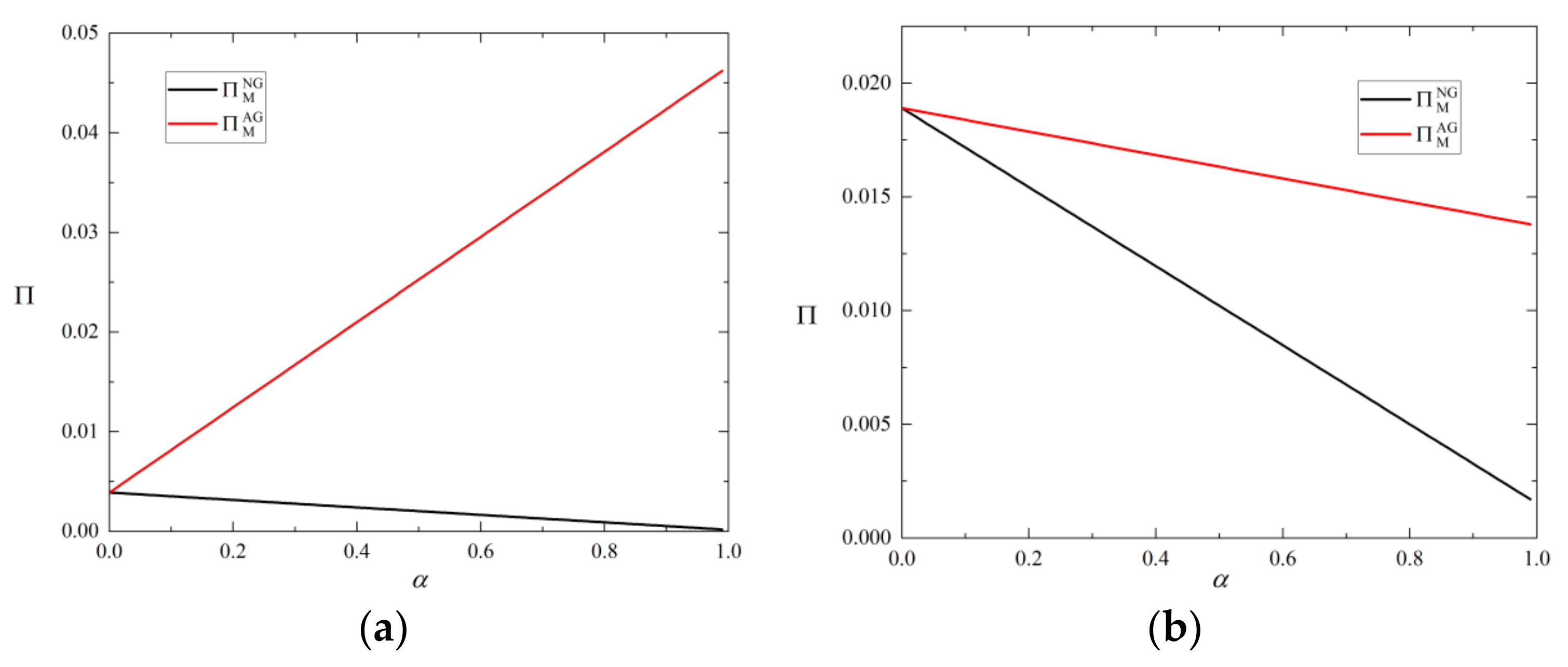
(1) Under EPR regulations, authorizing third parties to recycle used products is better for the manufacturers when the residual value coefficient of the used products is large. The manufacturer not only profits from the new consumers as well as the original consumers but also recycles the used products from third-party recyclers to achieve production cost savings. The premise is that the cost of production and sales are moderate, and the manufacturer has a high capacity to recycle and treat used products. In the actual operation process, the manufacturer also needs to consider the specific measures in the government regulation, pay attention to the production cost of new products, and their own interests, and then decide whether to authorize a third-party recycler.
(2) When the government, as the decision maker, establishes a subsidy of a trade-in program and a fund for the disposal of used products when the environmental benefits are optimal, the decision of the manufacturer is strongly impacted. Especially under Model ACG, the manufacturer needs to pay more funds, the market conditions for the profit of the trade-in program are harsher, and part of the profit is transferred to the government. This leads to a sharp decline in manufacturer profit, which leads to manufacturers choosing not to authorize third parties to recycle used products, which is contrary to our original intention.
(3) When the government does not act as the decision maker, the demand of new consumers and the pricing of products are only related to the market structure and production cost. Then, for the original consumers, manufacturers need to create their own good reputation to increase the stickiness of the original consumers, thus enhancing their own profits and disposing of more used products in the environment for long-term development.

6.2. Practical Implications

This paper studied the optimal strategies of the government and the manufacturer under the fund regulation mechanism. We determined the optimal trade-in subsidy and waste product disposal fund from the government’s perspective. From the manufacturer’s perspective, we studied the manufacturer’s optimal authorization strategy for third-party recycling. It aimed to actively promote the recycling and remanufacture of used products, reduce pollution emissions to the environment, constantly expand the influence of recycled products in consumer groups, and promote the production and use of recycled products.

6.3. Theoretical Contribution

This study has two main theoretical contributions. First, unlike remanufactured products, which were emphasized in much literature, this paper focused on recycling raw materials used to manufacture remanufactured products. Secondly, this paper subdivided consumers, used consumer function to describe the heterogeneity of consumers, and added consumer utility function to the brand product perception coefficient, which is more relevant to real life and provides guidance for manufacturers to make recycling decisions.

6.4. Limitations and Future Research Avenues

(1) In real life, due to the rapid changes in the supplier channel structure and market competition patterns, the profit function of third-party recyclers is relatively simply portrayed in this study, but we can still take the next step to use the complexity of the supplier structure that can increase its complexity to conduct more extensive market research so that the constructed model can be further adapted to the real decision-making environment to obtain more accurate and profound management insights.
(2) First, we assumed that manufacturers dominate the supply chain, but, in real life, retailers and recyclers are increasingly dominant, and many have become no less or even more dominant than manufacturers. Second, more often than not, no absolute dominant player exists in the supply chain; therefore, in-depth studies can be conducted in the future on the supply chain without a dominant player.
(3) We only focused on exploring the homogeneous prices of new and remanufactured products; in the future, heterogeneous and heterogeneous prices and even random substitution can be examined.

Author Contributions

Writing—original draft preparation, X.G.; writing—review and editing, J.C.; supervision, J.L. and Z.B. All authors have read and agreed to the published version of the manuscript.

Funding

This research was financially supported by the National Natural Science Foundation of China (72274175, 71874159).

Data Availability Statement

All relevant data are included in the paper.

Conflicts of Interest

The authors declare no conflict of interest.

Appendix A

In Model N, the Hesse matrix of the manufacturer’s profit function is: H M N = 2 Π M N p n 2 2 Π M N p n p t 2 Π M N p t p n 2 Π M N p t 2 . The values of each determinant are: 2 Π M N p n 2 = 2 1 α 2 α β δ u < 0 , 2 1 α 2 α β δ u 2 α β δ u 2 α β δ u 2 α β δ u = 4 α 1 α β δ u > 0 . We can judge that the Hesse matrix is a negative definite matrix. According to it nature, if the Hesse matrix is a negative definite matrix, a maximum exists, so an optimal solution exists to maximize the manufacturer’s profit. We obtain the manufacturer’s optimal solution thus: p n N = 1 + c n + f 2 ; p t N = 1 β + Δ + δ u s 2 . Substituting the optimal solution into Equations (1), (2) and (7), the optimal solution in Table 1 can be obtained.

Appendix B

Given q N N = 1 α 1 c n f 2 > 0 , q O N = α 1 2 c r + f s 2 β δ u > 0 , c n + f < 1 , β δ u c r f + s > 0 ; additionally, p n N p t N f c r = β + s δ u c r f 2 , then β δ u c r f + s > 0 .
q N N c n = 1 α 2 < 0 , q N N f = 1 α 2 < 0 , q O N c r = α 1 2 β δ u < 0 , q O N _ f = α 1 2 β δ u < 0 , q O N s = α 1 2 β δ u > 0 , q O N β = α c r + f s 2 β δ u 2 > 0 , q O N δ u = α c r + f s 2 β δ u 2 < 0 , Π M N c n = 1 α 1 c n f 2 < 0 , Π M N c r = α β δ u c r + s f 2 β δ u < 0 , Π M N s = α β δ u c r + s f 2 β δ u > 0 , Π M N δ u = α β δ u c r f + s β δ u + c r s + f 4 β δ u 2 < 0 , Π M N β = α β δ u c r f + s β δ u + c r s + f 4 β δ u 2 > 0 , Π M N f = 1 α 1 c n f 2 α β δ u c r + s f 2 β δ u < 0 .

Appendix C

Solve the game problem in Section 4.1.2 using backward induction method.
Substituting the above q N N and q O N into Equation (10), we obtain:
Π G N G = q O N e s N G + f N G + q N N f N G
The Hesse matrix of the government environmental benefit function can be obtained as follows: H G N G = 2 Π G N G s 2 2 Π G N G s f 2 Π G N G f s 2 Π G N G f 2 . The values of each determinant are as follows: 2 Π G N G s 2 = α β δ u < 0 , α β δ u α β δ u 2 α β δ u 1 α α β δ u = 1 α α β δ u > 0 .
We can judge that the Hesse matrix is a negative definite matrix. According to its nature, if the Hesse matrix is a negative definite matrix, a maximum exists, so an optimal solution exists to maximize the government’s profit. The optimal solution of the government is found as follows: s N G = 1 β + δ u Δ + e 2 ; f N G = 1 c n 2 . Substituting the optimal solution into Equations (1), (2), (7), (8), (9), and (10), the optimal solution in Table 5 can be obtained.

Appendix D

In Model A, the reaction function of the third-party is first obtained, and the second-order condition in Equation (13) is obtained 2 Π T A p u A = α 2 δ u . The second-order is less than zero, and a unique optimal solution theoretically exists. Therefore, the third-party reaction function can be obtained from the first-order condition Π M A p u A = α b A 2 p u A δ u = 0 and the reaction function is p u A = b A 2 . We substitute this reaction function into the manufacturer’s profit function. Thus, for a given b A , the manufacturer’s problem is m a x p n A , p t A Π M A .
The Hesse matrix of the manufacturer’s profit function is H M A = 2 Π M A p n 2 2 Π M A p n p t 2 Π M A p t p n 2 Π M A p t 2 . The values of each determinant are: 2 Π M A p n 2 = 2 1 α 2 α β δ u < 0 , 2 1 α 2 α β δ u 2 α β δ u 2 α β δ u 2 α β δ u = 4 α 1 α β δ u > 0 . We can judge that the Hesse matrix is a negative definite matrix. According to its nature, if the Hesse matrix is a negative definite matrix, a maximum exists, so an optimal solution exists to maximize the manufacturer’s profit. The manufacturer’s optimal solution is obtained as p n A b A = 1 + c n + f 2 ; p t A b A = 1 β + Δ + δ u s 2 . Substituting p n A b A , p t A b A , and p u A b A into Equation (14), we obtain:
m a x p n , p t Π M A = 1 α 1 c n f 2 2 + α β δ u + s c r f 2 4 β δ u + Δ b A α b A 2 δ u
According to 2 Π M A b 2 = α 1 δ u < 0 ; that is, the second order is less than zero and the function has a maximum value. So, an optimal solution exists to maximize the profit of the third-party recycler. According to the first-order condition Π M A b A = α 2 b A c n + c r 2 δ u = 0 , b A = c n c r 2 = Δ 2 . By substituting the optimal solution b A into Equations (3), (4), (13) and (14), the optimal solution in Table 6 is obtained.

Appendix E

Given q N A = 1 α 1 c n f 2 > 0 , q O A = α 1 2 c r + f s 2 β δ u > 0 , then c n + f < 1 , β δ u c r f + s > 0 ; additionally, p n A p t A f c r = β + s δ u c r f 2 , then β δ u c r f + s > 0 .
q N A c n = 1 α 2 < 0 , q N A f = 1 α 2 < 0 , q O A c r = α 1 2 β δ u < 0 , q O A f = α 1 2 β δ u < 0 , q O A s = α 1 2 β δ u > 0 , q O A β = α c r + f s 2 β δ u 2 > 0 , q O A δ u = α c r + f s 2 β δ u 2 < 0 , q T A c n = α 1 4 δ u > 0 , q T A c r = α 1 4 δ u < 0 , q T A δ u = α Δ 4 δ u 2 < 0 , Π M A c n = 1 α 1 c n f 2 + α Δ 4 δ u , c n < 2 δ u 1 α 1 f + α c r 2 δ u 1 α + α , Π M A c n < 0 , c n > 2 δ u 1 α 1 f + α c r 2 δ u 1 α + α , Π M A c n > 0 , Π M A c r = α β δ u c r + s f 2 β δ u α Δ 4 δ u < 0 , Π M A s = α β δ u c r + s f 2 β δ u > 0 , Π M A δ u = α β δ u c r f + s β δ u + c r s + f 4 β δ u 2 Δ 2 8 δ u 2 < 0 , Π M A β = α β δ u c r f + s β δ u + c r s + f 4 β δ u 2 > 0 , Π M A f = 1 α 1 c n f 2 α β δ u c r + s f 2 β δ u < 0 , Π T A c n = α Δ 8 δ u > 0 , Π T A c r = α Δ 8 δ u < 0 , Π T A δ u = α Δ 2 16 δ u 2 < 0 .

Appendix F

Solve the game problem in Section 4.2.2 using backward induction.
Substituting the above q N A , q O A and q T A into Equation (15), we obtain:
Π G A G = q O A + q T A e s A G + f A G + q N A f A G
The Hesse matrix of the government environmental benefit function can be obtained as: H G A G = 2 Π G A G s 2 2 Π G A G s f 2 Π G A G f s 2 Π G A G f 2 .
The values of each determinant are: 2 Π G A G s 2 = α β δ u < 0 , α β δ u α β δ u 2 α β δ u 1 α α β δ u = 1 α α β δ u > 0 .
We can judge that the Hesse matrix is a negative definite matrix. According to its nature, if the Hesse matrix is a negative definite matrix, a maximum exists, so an optimal solution exists to maximize the government’s profit. The optimal solution of the government is obtained as: s A G = Δ 4 δ u β Δ 4 + e + 1 β + δ u 2 ; f A G = 1 c n 2 . Substituting the optimal solution into Equations (3), (3), (13), (14) and (15), the optimal solution in Table 8 can be obtained.

Appendix G

In Model AC, the reaction function of the third party is first obtained, and the second-order condition in Equation (18) is obtained. The second-order 2 Π T A C p u A C = α 2 β is less than zero, and a unique optimal solution theoretically exists. Therefore, the third-party reaction function can be obtained from the first-order condition Π M A C p u A C = α b A C p n A C + p t A C + s 2 p u A C β = 0 , and the reaction function is p u A C = b A C p n A C + p t A C + s 2 . We substitute this reaction function into the manufacturer’s profit function. Thus, for a given b A C , the manufacturer’s problem is m a x p n A C , p t A C Π M A C .
The Hesse matrix of the manufacturer’s profit function is: H M A C = 2 Π M A C p n 2 2 Π M A C p n p t 2 Π M A C p t p n 2 Π M A C p t 2 . The values of each determinant are: 2 Π M A C p n 2 = 2 1 α α β < 0 , 2 1 α α β α β α β α β = 2 α 1 α β > 0 . We can judge that the Hesse matrix is a negative definite matrix. According to the nature of the Hesse matrix, if the Hesse matrix is a negative definite matrix, a maximum exists, so an optimal solution exists to maximize the manufacturer’s profit. The manufacturer’s optimal solution is obtained as: p n A C b A C = 1 + c n + f 2 ; p t A C b A C = 1 2 β s + 2 b A C 2 . Substituting p n A C b A C , p t A C b A C and p u A C b A C into Equation (19), we obtain: m a x b A C Π M A C = 1 α 1 c n f 2 2 + Δ b A C α 1 2 + c n + f s 4 β + α 1 2 c n + f s 4 β c n f 2 c r + 2 β + s 2 b A C 2 . We obtain the first-order condition Π M A C b A C = α < 0 . Therefore, the manufacturer takes the maximum profit when b A C is equal to its lower bound. Plug in the constraint θ 3 θ 2 and obtain b β + δ u c n + 2 β s + f 4 β . Substituting the optimal solution b A C into Equations (5), (6), (18) and (19), the optimal solution in Table 9 can be obtained.

Appendix H

Given q N A C = 1 α 1 c n f 2 > 0 , q O A C = α 1 2 c n + f s 4 β > 0 ; therefore, c n + f < 1 , 2 β c n f + s > 0 ; at the same time, p n A C p t A C f c r = Δ f + s + β δ u c r 2 c n + f s β + δ u 4 β . We can obtain 2 β c n f + s + β δ u 2 c r c n + f s β + δ u > 0 . q N A C c n = 1 α 2 < 0 , q N A C f = 1 α 2 < 0 , q O A C c n = α 1 4 β < 0 , q O A C f = α 1 4 β < 0 , q O A C s = α 1 4 β > 0 , q O A C β = α c n + f s 4 β 2 > 0 , q T A C c n = α 1 4 β > 0 , q T A C f = α 1 4 β > 0 , q T A C s = α 1 4 β < 0 , q T A C β = α c n + f s 4 β 2 < 0 , Π M A C c n = α β δ u + c n + f s 2 β 1 α 1 f c n 4 β , If α β δ u + c n + f s 2 β 1 α 1 f c n > 0 , then Π M A C c n > 0 ; If α β δ u + c n + f s 2 β 1 α 1 f c n < 0 , then Π M A C c n < 0 . Π M A C c r = α < 0 , Π M A C s = α 3 β + δ u c n + s f 4 β > 0 , Π M A C δ u = α 2 β + f + c n s 4 β < 0 , Π M A C β = α f + c n s f + c n s 2 δ u 8 β 2 < 0, Π M A C f = 2 β 2 β 1 α c n + f + α β + δ u c n f + s 4 β < 0 , Π T A C c n = α c n + 2 β s + f 8 β > 0 , Π T A C s = α c n + 2 β s + f 8 β < 0 , Π T A C f = α c n + 2 β s + f 8 β > 0 , Π T A C β = α c n + 2 β s + f 2 β c n + s f 16 β 2 > 0 .

Appendix I

Solve the game problem in Section 4.3.1 using backward induction.
Substituting the above q N A C , q O A C , and q T A C into Equation (20), we obtain Π G A C G = q O A C + q T A C e s A C G + f A C G + q N A C f A C G . By finding its first-order derivative, we find that Π G A C G s = α . In such a case, s takes the lower bound; that is, regardless of the subsidy provided to consumers by the government, based on the competitive relationship between the third-party recycler and the manufacturer and the original consumer utility function, the original consumers hand in their used products. Therefore, s A C G = 0 , 2 Π G A C G f 2 = 1 α < 0 . Hence, it must have unique optimal solution. Thus, we obtain the optimal solution from the first-order conditions Π G A C G f = 1 + α 1 α c n 2 f 1 α = 0 .

References

  1. Vanessa, F.C.P.B.; Ruediger, K.; Garam, B. The Global E-Waste Monitor. 2020. Available online: https://www.itu.int/pub/D-GEN-E_WASTE.01-2020 (accessed on 7 December 2020).
  2. Times, N.Y. Unwanted Electronic Gear Rising in Toxic Piles. Available online: https://blog.adafruit.com/2013/03/20/disposal-of-older-monitors-leaves-a-hazardous-trail/ (accessed on 7 December 2013).
  3. Esenduran, G.; Kemahlıoğlu-Ziya, E.; Swaminathan, J.M. Take-Back Legislation: Consequences for Remanufacturing and Environment. Decis. Sci. 2016, 47, 219–256. [Google Scholar] [CrossRef]
  4. Cao, J.; Chen, X.; Zhang, X.; Gao, Y.; Zhang, X.; Kumar, S. Overview of remanufacturing industry in China: Government policies, enterprise, and public awareness. J. Clean. Prod. 2020, 242, 118450. [Google Scholar] [CrossRef]
  5. Shittu, O.S.; Williams, I.D.; Shaw, P.J. Global E-waste management: Can WEEE make a difference? A review of e-waste trends, legislation, contemporary issues and future challenges. Waste Manag. 2020, 120, 549–563. [Google Scholar] [CrossRef]
  6. He, Q.; Wang, N.; Yang, Z.; He, Z.; Jiang, B. Competitive collection under channel inconvenience in closed-loop supply chain. Eur. J. Oper. Res. 2019, 275, 155–166. [Google Scholar] [CrossRef]
  7. Sheu, J.-B.; Choi, T.-M. Extended consumer responsibility: Syncretic value-oriented pricing strategies for trade-in-for-upgrade programs. Transp. Res. Part E Logist. Transp. Rev. 2019, 122, 350–367. [Google Scholar] [CrossRef]
  8. Khan, S.A.R.; Godil, D.I.; Thomas, G.; Tanveer, M.; Zia-Ul-Haq, H.M.; Mahmood, H. The Decision-Making Analysis on End-of-Life Vehicle Recycling and Remanufacturing under Extended Producer Responsibility Policy. Sustainability 2021, 13, 11215. [Google Scholar] [CrossRef]
  9. Alegoz, M.; Kaya, O.; Bayindir, Z.P. A comparison of pure manufacturing and hybrid manufacturing remanufacturing systems under carbon tax policy. Eur. J. Oper. Res. 2021, 294, 161–173. [Google Scholar] [CrossRef]
  10. Xiao, L.; Wang, X.-J.; Chin, K.-S. Trade-in strategies in retail channel and dual-channel closed-loop supply chain with remanufacturing. Transp. Res. Part E Logist. Transp. Rev. 2020, 136, 101898. [Google Scholar] [CrossRef]
  11. Cao, K.; Bo, Q.; He, Y. Optimal trade-in and third-party collection authorization strategies under trade-in subsidy policy. Kybernetes 2018, 47, 854–872. [Google Scholar] [CrossRef]
  12. Spicer, A.; Johnson, M. Third-party demanufacturing as a solution for extended producer responsibility. J. Clean. Prod. 2004, 12, 37–45. [Google Scholar] [CrossRef]
  13. Özdemir, Ö.; Denizel, M.; Guide, V.D.R. Recovery decisions of a producer in a legislative disposal fee environment. Eur. J. Oper. Res. 2012, 216, 293–300. [Google Scholar] [CrossRef]
  14. Esenduran, G.; Atasu, A.; Van Wassenhove, L.N. Valuable e-waste: Implications for extended producer responsibility. IISE Trans. 2019, 51, 382–396. [Google Scholar] [CrossRef]
  15. Chen, C.-K.; ‘Ulya, M.A. Analyses of the reward-penalty mechanism in green closed-loop supply chains with product remanufacturing. Int. J. Prod. Econ. 2019, 210, 211–223. [Google Scholar] [CrossRef]
  16. Chang, X.; Wu, J.; Li, T.; Fan, T.-J. The joint tax-subsidy mechanism incorporating extended producer responsibility in a manufacturing-recycling system. J. Clean. Prod. 2019, 210, 821–836. [Google Scholar] [CrossRef]
  17. Yan, Y.; Yao, F.; Sun, J. Manufacturer’s cooperation strategy of closed-loop supply chain considering corporate social responsibility. RAIRO Oper. Res. 2021, 55, 3639–3659. [Google Scholar] [CrossRef]
  18. Xing, E.; Shi, C.; Zhang, J.; Cheng, S.; Lin, J.; Ni, S. Double third-party recycling closed-loop supply chain decision under the perspective of carbon trading. J. Clean. Prod. 2020, 259, 120651. [Google Scholar] [CrossRef]
  19. Yu, Z.; Tianshan, M.; Khan, S.A.R. Investigating the effect of government subsidies on end-of-life vehicle recycling. Waste Manag. Res. 2021, 39, 860–870. [Google Scholar] [CrossRef]
  20. Zuqing, H.; Ronghua, Y.I.; Da, Q. Study on the Efficiency of the Closed-Loop Supply Chains with Remanufacture Based on Third-Party Collecting. Chin. J. Manag. Sci. 2008, 16, 73–77. [Google Scholar]
  21. Hong, X.; Xu, L.; Du, P.; Wang, W. Joint advertising, pricing and collection decisions in a closed-loop supply chain. Int. J. Prod. Econ. 2015, 167, 12–22. [Google Scholar] [CrossRef]
  22. Chu, X.; Zhong, Q.; Li, X. Reverse channel selection decisions with a joint third-party recycler. Int. J. Prod. Res. 2018, 56, 5969–5981. [Google Scholar] [CrossRef]
  23. Ray, S.; Boyaci, T.; Aras, N. Optimal Prices and Trade-in Rebates for Durable, Remanufacturable Products. Manuf. Serv. Oper. Manag. 2005, 7, 208–228. [Google Scholar] [CrossRef]
  24. Li, Y.; Feng, L.; Govindan, K.; Xu, F. Effects of a secondary market on original equipment manufactures’ pricing, trade-in remanufacturing, and entry decisions. Eur. J. Oper. Res. 2019, 279, 751–766. [Google Scholar] [CrossRef]
  25. Agrawal, V.V.; Ferguson, M.; Souza, G.C. Trade-In Rebates for Price Discrimination and Product Recovery. IEEE Trans. Eng. Manag. 2016, 63, 326–339. [Google Scholar] [CrossRef]
  26. Hu, S.; Ma, Z.-J.; Sheu, J.-B. Optimal prices and trade-in rebates for successive-generation products with strategic consumers and limited trade-in duration. Transp. Res. Part E Logist. Transp. Rev. 2019, 124, 92–107. [Google Scholar] [CrossRef]
  27. Hong, X.; Govindan, K.; Xu, L.; Du, P. Quantity and collection decisions in a closed-loop supply chain with technology licensing. Eur. J. Oper. Res. 2017, 256, 820–829. [Google Scholar] [CrossRef]
  28. Chen, Y.; Chen, F. On the Competition between Two Modes of Product Recovery: Remanufacturing and Refurbishing. Prod. Oper. Manag. 2019, 28, 2983–3001. [Google Scholar] [CrossRef]
  29. Mondal, C.; Giri, B.C. Pricing and used product collection strategies in a two-period closed-loop supply chain under greening level and effort dependent demand. J. Clean. Prod. 2020, 265, 121335. [Google Scholar] [CrossRef]
  30. Cao, J.; Wu, S.; Zhang, X.; Zhou, G. Corporate strategies on remanufacturing with EPR regulation. Control and Decision 2020, 35, 1703–1716. [Google Scholar]
Figure 1. Supply chain model composed of third-party recycler and manufacturer. (a) Model N (manufacturer does not authorize third-party recycler to recycle used products); (b) Models A and AC (manufacturer authorizes third-party recycler to recover used products).
Processes 11 00166 g001
Figure 2. Willingness of original consumers to pay in market under Model A.
Processes 11 00166 g002
Figure 3. Willingness of original consumers to pay in market under Model AC.
Processes 11 00166 g003
Figure 4. Impact of β on manufacturer profit. (a) s = 0.25 ; (b) s = 0.8 .
Processes 11 00166 g004
Figure 5. Profit of the manufacturer under Models NG and AG. (a) c n = 0.45 , (b) c n = 0.75 .
Processes 11 00166 g005
Figure 6. Profit of the manufacturer under Models NG and ACG. (a) c n = 0.45 , (b) c n = 0.75 .
Processes 11 00166 g006
Table 1. Comparison of this study with related studies.
AuthorsEPR RegulationTPRTrade-In ProgramConsumer SegmentationMethodology
Khan et al. [8] (1)
Ozdemir et al. [13] (4)
Esenduran et al. [14] (3) & (4)
Chang et al. [16] (2)
Hu et al. [26] (4)
Agrawal et al. [25] (4)
Xiao et al. [10] (2) & (4)
Zhang et al. [19] (3)
Li et al. [24] (3) & (4)
Our study(2) & (4)
(1) Evolutionary game theory; (2) Stackelberg game theory; (3) Cournot game theory; (4) optimization theory with constraints.
Table 2. Notations.
Table 2. Notations.
NomenclatureMeaning
c n Unit production cost of new product
c r Unit production cost of remanufactured products
β Value coefficient of branded product
δ u Residual value coefficient of used products
α Proportion of original consumers
θ Willingness of consumers to pay for new products
q N i ,   p n i Demand and price of products purchased by new consumers; i = N , A , A C , N G , A G , A C G
q O i ,   p n i Demand and price of products purchased by original consumers
q T i ,   p u i Demand and price of used products recovered by third-party recyclers
f Amount of government levy fund
b Transfer price of used products
p t i Discount price of used products
s Amount of government subsidy of trade-in programs
e Environmental benefit of used products
j i Manufacturer profit ( j = M ); hird-party profit ( j = T ); government benefit ( j = G )
Table 3. Optimal solution of Model N.
Optimal SolutionModel N
p n N 1 + c n + f 2
p t N 1 β + Δ s + δ u 2
q N N 1 α 1 c n f 2
q O N α 1 2 c r + f s 2 β δ u
Π M N 1 α 1 c n f 2 2 + α β + s δ u f c r 2 4 β δ u
Table 4. Monotonicity of q N N ,   q O N ,   and Π M N with respect to β ,   δ u ,   c n ,   c r ,   s , and f .
Variable q N N   q O N   Π M N  
β -
δ u -
c n -
c r -
s -
f
Explanation: ↗ means when the variable increases, the dependent variable increases; ↘ means when the variable increases, the dependent variable decreases; ”-” means the value is independent of the variable. The following arrows are the same.
Table 5. Equilibrium optimal solutions and optimal profits under Model NG.
Equilibrium s N G = 0
1 Δ + e < β δ u < 1 + Δ
s N G = 1 β + δ u Δ + e 2
c r e < β δ u < 1 Δ + e
p n N G 3 + c n 4 3 + c n 4
p t N G 1 β + Δ + δ u 2 1 β + 3 Δ e + δ u 4
q N N G 1 α 1 c n 4 1 α 1 c n 4
q O N G α 1 2 1 Δ + c r 4 β δ u α 1 4 c r e 4 β δ u
f N G 1 c n 2 1 c n 2
Π M N G 1 α 1 c n 4 2 + α 2 β 2 δ u 1 + Δ c r 2 16 β δ u 1 α 1 c n 4 2 + α β c r + e δ u 2 16 β δ u
Π G N G α 1 2 1 Δ + c r 4 β δ u e + 1 c n 2
+ 1 α 1 c n 2 8
α 1 4 c r e 4 β δ u e + β c r δ u 2
+ 1 α 1 c n 2 8
Table 6. Optimal solution of Model A closed-loop supply chain.
EquilibriumsModel A
p n A 1 + c n + f 2
p t A 1 β s + δ u + Δ 2
b A Δ 2
q N A 1 α 1 c n f 2
q O A α 1 2 c r + f s 2 β δ u
p u A Δ 4
q T A α Δ 4 δ u
Π M A 1 α 1 c n f 2 2 + α β + s δ u f c r 2 4 β δ u + α Δ 2 8 δ u
Π T A α Δ 2 16 δ u
Table 7. Monotonicity of q N A ,   q T A ,   q O A ,   Π M A , and Π T A regarding β ,   δ u ,   c n ,   c r ,   s , and f .
Variable q N A   q O A   q T A   Π M A   Π T A  
β ---
δ u -
c n -If c n > 2 δ u 1 α 1 f + α c r 2 δ u 1 α + α ,↗
If   c n < 2 δ u 1 α 1 f + α c r 2 δ u 1 α + α ,↘
c r -
s ---
f --
Explanation: ↗ means when the variable increases, the dependent variable increases; ↘ means when the variable increases, the dependent variable decreases; ”-” means the value is independent of the variable. The following arrows are the same.
Table 8. Equilibrium optimal solution and optimal profit under Model AG.
Equilibrium s A G = 0  
max 2 δ u 1 Δ + e 2 δ u + Δ , 1 + c r 2 < β δ u < 1 + Δ  
s A G = Δ 4 δ u β Δ 4 + e + 1 β + δ u 2  
2 c n e 2 δ u 2 δ u Δ < β δ u < 2 δ u 1 Δ + e 2 δ u + Δ  
p n A G 3 + c n 4 3 + c n 4
p t A G 1 β + Δ + δ u 2 Δ 8 δ u β + δ u + 1 + δ u β e + 2 Δ 4
p u A G Δ 4 Δ 4
q N A G 1 α 1 c n 4 1 α 1 c n 4
q O A G α 1 2 1 Δ + c r 4 β δ u α 1 4 c r Δ e 4 β δ u β + δ u Δ 8 δ u β δ u
f A G 1 c n 2 1 c n 2
Π T A G α Δ 2 16 δ u α Δ 2 16 δ u
Π M A G 1 α 1 c n 4 2 + α Δ 2 8 δ u + α 2 β 2 δ u 1 + Δ c r 2 16 β δ u 1 α 1 c n 4 2 + α Δ 2 8 δ u +
α 2 δ u β δ u c r + e β δ u Δ 2 64 δ u 2 β δ u
Π G A G α Δ 4 δ u + 1 2 1 Δ + c r 4 β δ u e + 1 c n 2 + 1 α 1 c n 2 8 1 α 1 c n 2 8 + α 2 δ u β δ u + e c r + β δ u Δ 2 32 δ u 2 β δ u
Table 9. Optimal solution of Model AC closed-loop supply chain.
EquilibriumModel AC
p n A C 1 + c n + f 2
p t A C 2 2 β + c n + f 3 s 4 + δ u c n + 2 β s + f 4 β
b A C β + δ u c n + 2 β s + f 4 β
q N A C 1 α 1 c n f 2
q O A C α 1 2 c n + f s 4 β
p u A C δ u c n + 2 β s + f 4 β
q T A C α 1 2 + c n + f s 4 β
Π M A C 1 α 1 c n f 2 2 + α Δ β + δ u c n + 2 β s + f 4 β 1 2 + c n + f s 4 β  
+ α 1 2 c n + f s 4 β Δ f + s + β δ u c r 2 c n + f s β + δ u 4 β
Π T A C α c n + 2 β s + f 2 16 β
Table 10. Monotonicity of q N A C ,   q O A C ,   q T A C ,   Π M A C , and Π T A C with respect to β ,   δ u ,   c n ,   c r ,   s , and f .
Parameter q N A C   q O A C   q T A C   Π M A C   Π T A C  
β -If f + c n s f + c n s 2 δ u < 0 ,↗
If   f + c n s f + c n s 2 δ u > 0 ,↘
δ u ----
c n If α β δ u + c n + f s 2 β 1 α 1 f c n > 0 , ↗
If α β δ u + c n + f s 2 β 1 α 1 f c n < 0 , ↘
c r ----
s -
f
Explanation: ↗ means when the variable increases, the dependent variable increases; ↘ means when the variable increases, the dependent variable decreases; ”-” means the value is independent of the variable. The following arrows are the same.
Table 11. Optimal solutions of Model ACG_III closed-loop supply chain.
EquilibriumModel ACG
p n A C G 3 + c n 4 + α 2 1 α
p t A C G 1 2 1 β + δ u + c n β + δ u 8 β + 1 + α β + δ u 8 β 1 α
b A C G β + δ u 1 + c n + 4 β 1 α + 2 α 8 β 1 α
q N A C G 1 α 1 c n 4 1 2 α
q O A C G α 1 2 + 1 + c n 1 α + 2 α 8 β 1 α
p u A C G 2 β + c n 4 β δ u
q T A C G α 1 2 1 + c n 1 α + 2 α 8 β 1 α
Π M A C G 1 c n 1 α 3 α 2 16 1 α + α 1 2 + 1 + c n 1 α + 2 α 8 β 1 α Δ β + δ u c n 1 α + 4 β 1 α + 1 + α 8 β 1 α + α 1 2 1 + c n 1 α + 2 α 8 β 1 α 4 β + 5 c n 8 c r 1 α 3 1 + α 8 1 α δ u c n + 4 β + 1 1 α + 2 α 8 β 1 α
Π T A C G α 1 + c n + 4 β 1 α + 2 α 2 64 β 1 α
Π G A C G α e + 1 c n 2 + α 1 α + 1 α 1 c n 4 1 2 α 1 c n 2 + α 1 α
Disclaimer/Publisher’s Note: The statements, opinions and data contained in all publications are solely those of the individual author(s) and contributor(s) and not of MDPI and/or the editor(s). MDPI and/or the editor(s) disclaim responsibility for any injury to people or property resulting from any ideas, methods, instructions or products referred to in the content.

