A Bearing Fault Diagnosis Method Based on Spectrum Map Information Fusion and Convolutional Neural Network

Abstract

With the development of information technology, it has become increasingly important to use intelligent algorithms to diagnose mechanical equipment faults based on vibration signals of rolling bearings. However, with the application of high-performance sensors in the Internet of Things, the complexity of real-time classification of multichannel, multidimensional sensor signals is increasing. In view of the need for intelligent methods for fault diagnosis methods of mechanical equipment, the generalization ability of fault diagnosis models also needs to be further strengthened. In this context, in order to make fault diagnosis intelligent and efficient, a bearing fault diagnosis method based on spectrum map information fusion and convolutional neural network (CNN) is proposed. First, short-time Fourier transform (STFT) is used to analyze the multichannel vibration signal of the rolling bearing and obtain the frequency domain information of the signal over a period of time. Second, the information fusion is converted into two-dimensional (2D) images, which are input into CNN for training, and the bearing fault identification model is obtained. Next, the frequency domain information of each signal is converted into a 2D spectrum map, which is used as a CNN training dataset to train a bearing fault identification model. Finally, the diagnostic model is validated using the existing datasets. The results show that the accuracy of fault diagnosis using the proposed bearing is greater than 99.4% and can even reach 100%. The proposed method considerably reduces the workload of the diagnosis process, with strong robustness and generalization ability.

1. Introduction

Rolling bearings are an important part of rotating mechanisms and are widely used in industrial equipment and transportation equipment in various fields. Bearings are also the most vulnerable part to damage in mechanical equipment, reflecting the health of mechanical components. Studies show that bearing defects account for 40% of faults in large machinery and 90% of faults in small machinery [1,2,3,4]. At present, rolling bearings generally lack real-time state monitoring and fault diagnosis during the operation process, and equipment maintenance generally depends on manual experience, which is associated with considerably uncertainty; if faults cannot be dealt with in time, the service life of the equipment can be considerably reduced. Vibration generated during the operation of rolling bearings can reflect the health status of equipment. Real-time monitoring of vibration signals during the operation of bearings is a common method to judge the condition of equipment [5,6,7,8].

Rolling bearings exist in large numbers in mechanical equipment with rotating mechanisms and are widely used in industrial equipment and transportation equipment in various fields. Bearings are also the most vulnerable part to damage in mechanical equipment, reflecting the health of mechanical components. Studies have shown that 40% of large mechanical failures are caused by bearing failures, and such failures account for as much as 90% of the failure causes of small mechanical equipment [1,2,3,4]. At present, mechanical equipment generally lacks real-time health assessment and fault diagnosis for rolling bearings. The maintenance of mechanical equipment generally relies on manual experience, which is associated with considerable uncertainty. Failure to deal with faults in time can considerably reduce the service life of equipment. Vibration generated during the operation of rolling bearings can reflect the health status of equipment. Real-time monitoring of vibration signals during the operation of bearings is a common method to judge the condition of equipment [5,6,7,8].

The diagnosis of vibration signals initially relies on the judgment of manual experience to estimate the health of equipment. This method is suitable for small mechanical equipment, but in the face of multimechanism combinations of mechanical systems, such a method cannot be relied upon to make a correct judgment. Therefore, more intelligent diagnosis methods need to be further developed. The core of traditional intelligent diagnosis methods is feature extraction and classification following signal acquisition. Many researchers have investigated the use of bearing signals to diagnose the health status of mechanical equipment and have achieved important results [9,10,11,12,13,14]. Wu et al. [15] proposed an improved quantum-excited differential evolution algorithm using Mexh wavelet function to improve the global search ability of the algorithm and avoid the problem of excessively rapid convergence of the algorithm. Compared with other comparison methods, Wu et al. achieved better optimization performance in rolling bearing vibration data classification. Ali et al. [16] proposed a new indicator to improve fault detection ability by considering all frequency bands with valuable diagnostic information by combining square envelope spectra. Yi et al. [17] diagnosed local faults of rolling bearings by extracting pulse features. Haidong et al. [18] proposed a new intelligent method for fault diagnosis of rolling bearings called integrated depth autoencoder (EDAE), which overcame the dependence on manual feature extraction.

Using the traditional signal analysis method can preliminarily solve the bearing fault diagnosis problem. However, in modern industry, large mechanical and electrical equipment has become increasingly complex and is required to run continuously under different working conditions. The data generated also presents new characteristics, such as large quantity, variety and complex form. With the continuous progress of intelligent algorithms, convolutional neural networks have been used to diagnose vibration signals in recent years [19,20,21,22,23,24]. Levent et al. [25] used a one-dimensional (1D) convolutional neural network for real-time diagnosis of bearing faults, with the characteristics of compact structure and self-adaptation. Duy-tang et al. [26] used the method of directly inputting the vibration signal into a deep learning algorithm without using any feature extraction technology and achieved high diagnostic accuracy and robustness in a noisy environment. Liang et al. [27] used a deep convolutional transfer learning network to diagnose bearing faults with fewer samples in order to cope with the problem of insufficient data.

At present, most of researchers are using 1D bearing vibration signal recognition directly, whereas fewer researchers are turning the 1D vibration signal into a 2D signal to make full use of the neural network for identification of 2D image feature extraction ability, which has achieved a higher recognition accuracy. However, there are still some shortcomings with respect to training time, complexity and recognition for diagnosis with small sample datasets [28,29,30,31,32]. Therefore, in this paper, we propose a bearing fault diagnosis method based on spectrum map information fusion and a convolutional neural network. First, the 1D signal is converted into a 2D spectrum map using STFT. Under the condition of limited sample data, several mainstream convolutional neural network architectures are compared, and the VGG (Visual Geometry Group) neural network is selected as the training network. Finally, the lowest 99.4% and the highest 100% fault diagnosis accuracies are obtained in a test on the Case Western Reserve University (CWRU) dataset, and 99.8% fault diagnosis accuracy is also obtained in a test on different datasets, which shows that the method can effectively diagnose bearing faults according to the vibration signal and obtain good results with different datasets.

2. Methods

2.1. VGG Convolutional Neural Network (CNN)

Current mainstream CNN models include AlexNet, GoogLeNet and the VGG network. Among them, the VGG network proposed by the Visual Geometry Group of Oxford University in 2014 is a neural network applied in image classification and recognition, with excellent feature extraction capabilities. The network contains 13 convolutional layers and 3 fully connected layers. VGG stacks multiple $3\times 3$ convolution kernels to replace the large convolution kernels in traditional neural networks. Multiple convolution kernels effectively expand the number of channels. The pooling layer is used to reduce the width and height, making the constructed neural network more efficient, deeper, wider and less computationally intensive for large-scale neural networks [33]. The VGG network uses the ReLU function as the activation function. Unlike the Tanh and Sigmoid functions, the ReLU function is an unsaturated function, which means that it does not reduce the error of backpropagation, and the network converges faster, which can considerably reduce the training time. Based on these advantages, the fault diagnosis model uses the VGG network structure, which is shown in Figure 1.

There was an excessive number of weight parameters of VGG-16, with three full-connection layer parameters accounting for a large proportion. The original parameter setting of VGG-16 was to complete 1000 classifications, with fewer signal classifications. Therefore, the first two fully connected layers only use half of the original number of nodes, namely 2048 nodes, and the third fully connected layer has 10 nodes corresponding to the classification category so as to improve the recognition accuracy and efficiency of the model.

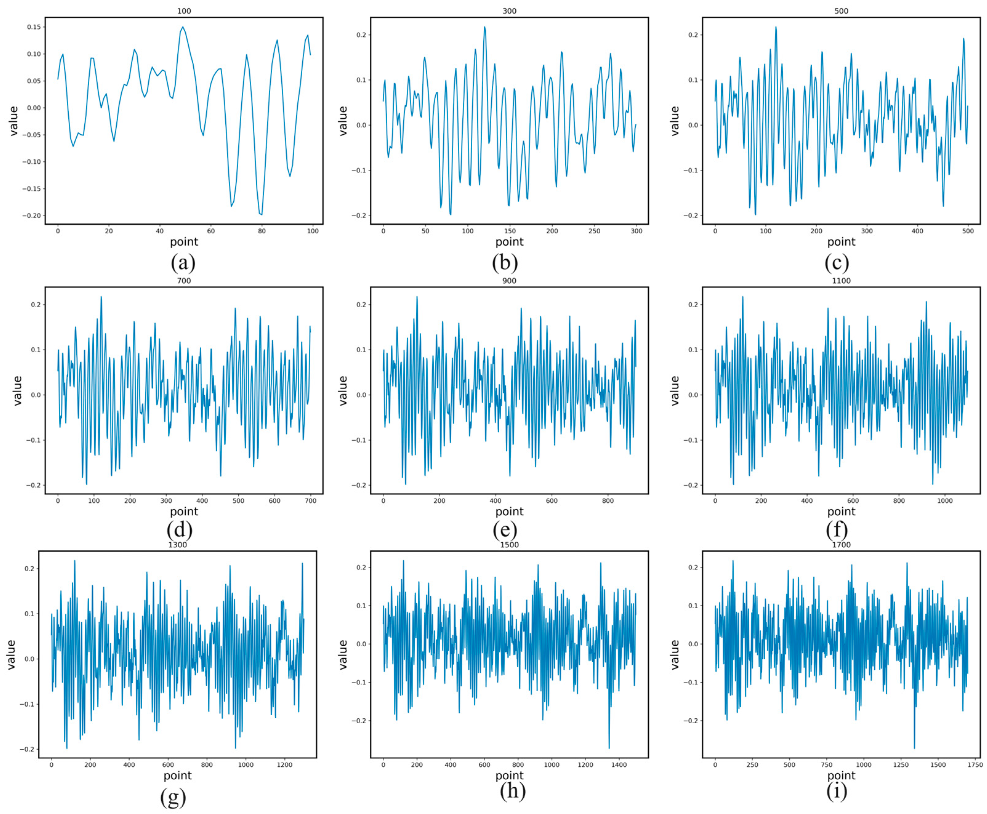
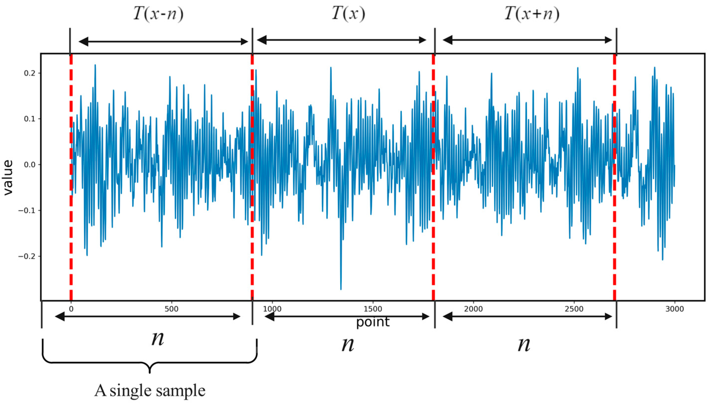
2.2. Data Segmentation

The vibration signal of the bearing is a continuous 1D time series, so different data segmentation methods should be selected according to the signal type. The vibration signals should be sequentially and equally intercepted into different small segments, and the signal interval of each segment should be long enough to capture the local features of the signal. However, the number of sampling points in the original dataset is fixed; the more sampling points each sample contains, the fewer the samples. A smaller number of samples is not conducive to training of neural networks. Before the experiment, the influence of samples with different data length pairs on the results should be tested, and the optimal data segmentation length should be selected according to the model recognition accuracy [34,35]. The main dataset is the bearing vibration data from the CWRU dataset, using the single-channel drive-end (DE) accelerometer data.

For determination of data length, the data are not processed, and 2D images are drawn directly by the matplotlib function. The obtained datasets are shown in

Table 1. Training set and verification set.

Class	Nor	IR0.007	B0.007	OR0.007	IR0.014	B0.014	OR0.014	IR0.021	B0.021	OR0.021
Train	2196	1091	1102	1097	1096	1096	1095	1098	1098	1102
Val	243	121	122	121	121	121	121	121	121	122

, and 9 signals of different lengths are shown in Figure 2. A total of 9 groups of datasets of different lengths are tested, i.e., 100, 300, 500, 700, 900, 1100, 1300, 1500 and 1700. The number of datasets constructed by 9 different sample lengths is the same, and the specific number is given in Table 1. The number of concrete can be divided into 10 categories: normal; inner race, 0.007 mils; ball, 0.007 mils; outer race, 0.007 mils; inner race, 0.014 mils; ball, 0.014 mils; outer race, 0.014 mils; inner race, 0.021 mils; ball, 0.021 mils; outer race, 0.021 mils.

Nine single-channel datasets of different lengths were trained using convolutional neural network training. The data length of a single sample in all subsequent experiments presented in this paper was ultimately determined according to the training results of single-channel DE datasets and the accuracy of bearing fault diagnosis of the obtained model. Figure 3 shows the training results; the precision of training increases with an increased number of data points. However, when a single sample contains more than 900 data points, the precision of the model declines, and loss function values begin to change. Therefore, 900 data points were chosen as a sample.

After the length of each sample is determined, the data are divided according to the time series, as shown in Formula (1). The signal intervals do not overlap; $x$ is the current time point, and n is the selected signal interval length.

$$T\left(x-n\right)\le T\left(x\right)\le T\left(x+n\right) x\in \left(n,2n,\dots ,xn\right)$$

(1)

A data segment after segmentation is shown in Figure 4. When 900 data points are divided into one sample, each sample is guaranteed to contain a cycle and comprehensive fault features.

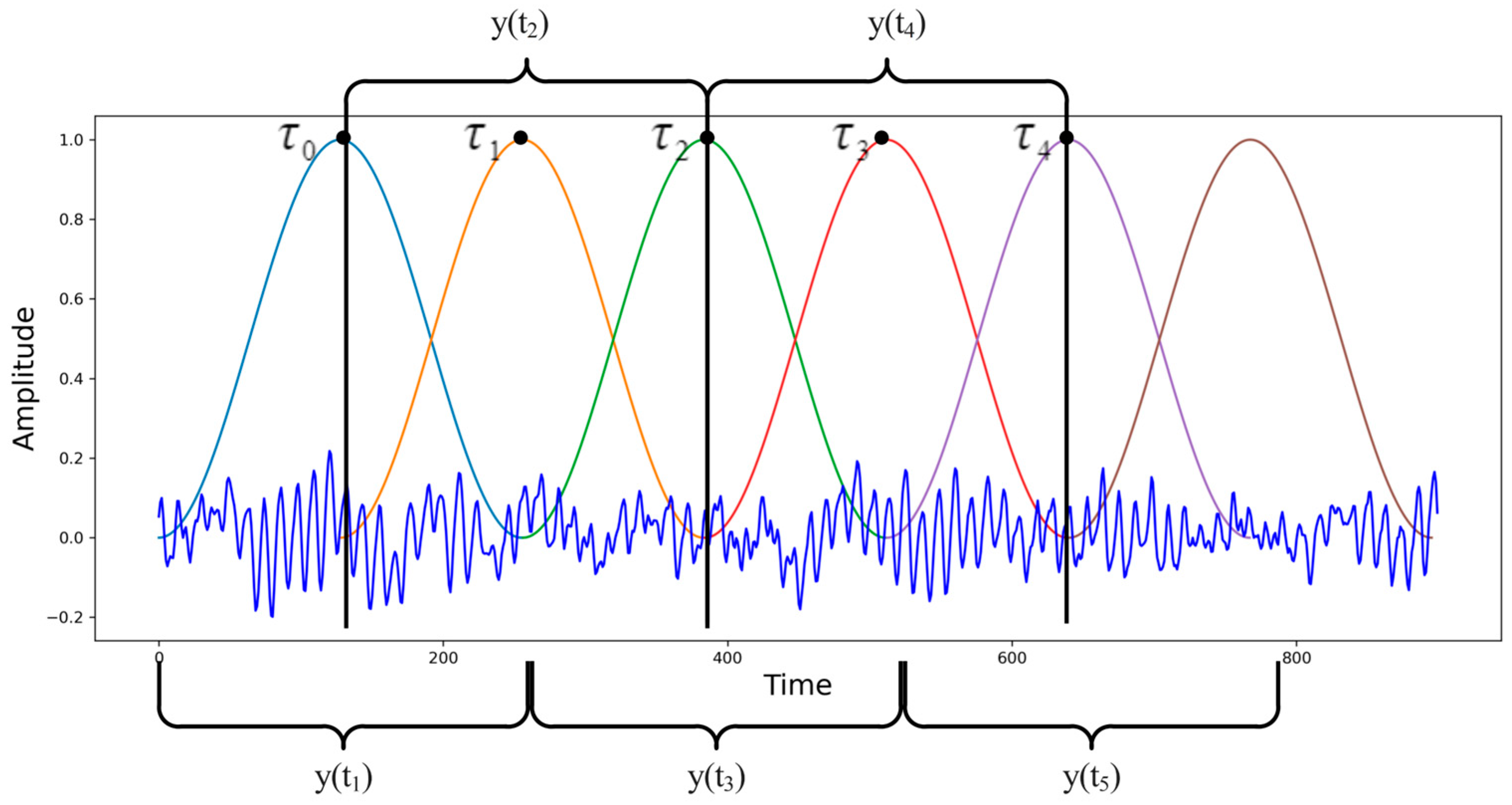
2.3. Spectral Analysis of Short-Time Fourier Transform (STFT)

Fourier transform can decompose a signal into several frequency components; each sinusoidal component has its own frequency and amplitude. Fourier transform can only determine which frequency components a signal contains for a period of time, but it cannot accurately determine the time when each frequency component appears. Therefore, it is possible to obtain similar spectrograms by analyzing signal fragments in different time domains. Therefore, Fourier transform is not suitable for signals with irregular periodic changes. The bearing vibration signal is a non-stationary signal containing different frequency components.

Therefore, it is not simple to use Fourier transform to analyze the spectrum of the signal. In order to avoid the loss of time information by Fourier transform of the entire sequence, local frequency parameters can be introduced, and Fourier transform can be used locally in the signal. By adding a window to intercept the segment of the signal, a window function ($w\left(t\right)$) is defined, as in Formula (2). The window function is moved to a certain center point ($\tau$) and multiplied by the original signal to obtain the truncated signal ($y\left(t\right)$).

$$y\left(t\right)=x\left(t\right)w\left(t-{\tau }_0\right)$$

(2)

Then, Fourier transform is used to analyze the truncated signal ($y\left(t\right)$) and obtain the spectral distribution ($X\left(\omega \right)$) of a segmented sequence according to Formula (3).

$$X\left(\omega \right)=F\left(y\left(t\right)\right)={{\displaystyle \int }}_{-\infty }^{+\infty }x\left(t\right)w\left(t-{\tau }_0\right)e^{-j\omega t}dt$$

(3)

In real applications, because the signal is a discrete point sequence, the spectrum sequence ($X\left[N\right]$) is obtained. For the convenience of expression, we define the function $S\left(\omega , \tau \right)$ in Formula (4), which represents the spectral result ($X\left(\omega \right)$) after transforming the original function when the center of the window function is $\tau$ [36].

$$S\left(\tau ,\omega \right)=F\left(x\left(t\right)w\left(t-\tau \right)\right)={{\displaystyle \int }}_{-\infty }^{+\infty }x\left(t\right)w\left(t-\tau \right)e^{-j\omega t}dt$$

(4)

Corresponding to the discrete scene, $S\left(\omega ,\tau \right)$ is a two-dimensional matrix, and each column represents the result sequence of windowing the signal at different positions and performing Fourier transform on the obtained signal segment. After completing the Fourier transform operation of the first segment, the window function is moved to ${\tau }_0$, and the moving distance is generally less than the width of the window so as to ensure that there is a certain overlap between the two windows before and after, which we call overlap. The above operations are repeated, and the window is continuously slid to perform Fourier transform on the data truncated by the window to obtain the spectral results ($S\left(\omega ,\tau \right)$) of all segments from ${\tau }_0$ to ${\tau }_N$ [37,38], as shown in Figure 5.

The result of Fourier transform of each window is a complex two-dimensional matrix; each column of this matrix is the spectrum of a window, and the number of columns in the matrix is equal to the number of segments of the signal divided by the window. This is used to determine the magnitude of the complex number to obtain the real amplitude value; then, the color block is used to represent the amplitude of each column. The higher the amplitude, the brighter the color block, and the lower the amplitude, the darker the color block, the specific operation process is shown in Figure 6.

In this study, we used the pcolormesh() function in the matplotlib library to draw the spectrogram. The Hanning window is used as the window function. The Hanning window is suitable for non-periodic continuous signals to reduce the leakage phenomenon and improve the quality of the spectrum analysis. Formula (5) is the time domain expression for the length of the Hanning window. The length of the window function is set to 256, with an overlap of 50%. The time-domain signal is then divided into segments using a sliding window.

$$w\left(n\right)=\frac{1}{2}\left[1-\cos (\frac{2\pi n}{N})\right] n=0,1,2,\cdots ,\mathrm{N}-1$$

(5)

Figure 7 shows an effect diagram after coding. The STFT diagram is obtained when the upper part is divided into vibration data of a single channel and the lower part is divided into vibration data of two channels. The STFT matrices of the two channels are obtained and added together.

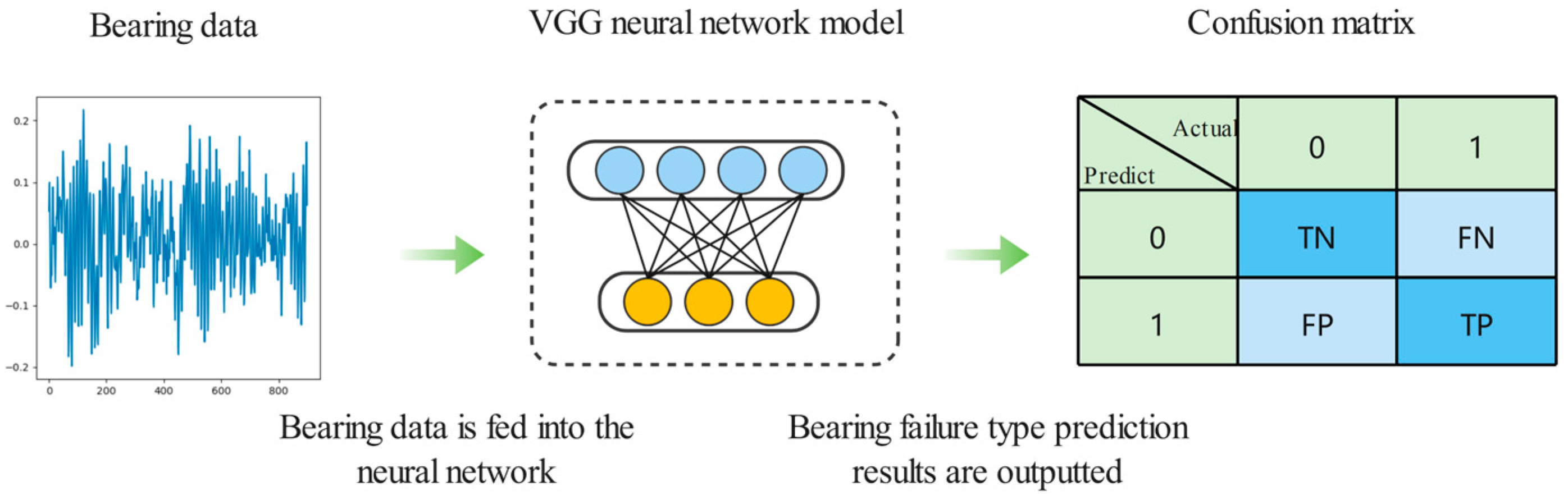
2.4. Diagnostic Methods

The process of bearing fault diagnosis based on spectrum map information fusion and convolutional neural network proposed in this paper is shown in Figure 8. First, according to the intercept signal and signal segment of a certain length, an appropriate method is selected based on 1D vibration signal processing to convert a signal fragment to a 2D spectrum map. Then, the spectrum map dataset is divided into a training set and a validation set according to a certain proportion. The training set is input into VGG for training, and the validation set is input into the model to predict the fault type. The specific steps are as follows.

• Sensors installed in different locations of the equipment collect vibration signals. In this study, we used collected vibration datasets rather than real-time vibration signals.
• The collected vibration signals are processed, the appropriate length is selected as a sample and 1D data are processed by the STFT method. The processed 1D data are stored as 2D images by Matplotlib. When the dataset is multidimensional, a multichannel dataset is generated by data fusion to improve the recognition accuracy.
• The spectrum map dataset is divided into a training set and a validation set according to a certain proportion.
• Appropriate neural networks are selected for training. Finally, a VGG convolutional neural network is used to train the model on the training set to obtain the neural network prediction model of bearing faults.
• The trained model is deployed to mechanical equipment for fault detection.

3. Dataset

In this study, two public bearing vibration datasets were selected, namely multi-channel, multicondition and single-channel datasets. Comparative experiments were conducted in two datasets. First, a single-channel data validation approach was used in dataset 1. Then, the number of channels of data was increased to observe the influence of the channel number on diagnosis accuracy. Finally, the generalization ability of the method under different working conditions was verified using vibration data under different bearing loads. In dataset 2, a single-channel dataset was used to generate a spectrum map dataset for training and validation, and the generalization ability of the method under different hardware conditions was tested.

3.1. Dataset 1: Case Western Reserve University (CWRU) Dataset

The first dataset used in this paper is from the rolling bearing test bed of Case Western Reserve University in the U.S., which is mainly composed of motors, bearings and load motors [39]. The load motor is a Reliance 2 hp motor with vibration sensors mounted near the motor bearings and sampled at 12 kHz and 48 kHz sampling frequencies, Figure 9 shows the Case Western Reserve University rolling bearing test stand.

The dataset includes four different bearing vibration signals: normal state, inner ring fault, roller fault and outer ring fault. The faults are divided into three fault types, 0.007 mls, 0.014 mls and 0.021 mls, according to their severity, and the sampling frequency is 12 kHz. The vibration signal experiment is conducted when the corresponding speed is vibration information of DE (drive end accelerometer data) and FE (fan end accelerometer data) channels at 1797 r/min, 1772 r/min, 1750 r/min and 1730 r/min. In the actual training, there are 10 categories: normal; inner race, 0.007 mils; ball, 0.007 mils; outer race, 0.007 mils; inner race, 0.014 mils; ball, 0.014 mils; outer race, 0.014 mils; inner race, 0.021 mils; ball, 0.021 mils; outer race, 0.021 mils. The 10 classification datasets at 0 HP were taken as the main experimental object, and 1 HP, 2 HP and 3 HP were taken as the validation datasets for the final method.

3.2. Dataset 2: Society for Machinery Failure Prevention Technology (MFPT) Dataset

Dataset 2 is an open access dataset published by the Society for Machinery Failure Prevention Technology. The MFPT dataset classifies bearing faults into three categories— baseline conditions, outer race faults and inner race fault conditions—with outer-race faults containing two different fault types. In this study, the MFPT dataset is used to verify the generalization ability of fault diagnosis using spectrum maps. In actual training, the labels are divided into four categories: baseline conditions, outer-race fault conditions, more outer-race fault conditions and inner-race fault conditions [40].

4. Experiment and Analysis

All experiments in described this paper were run on a Lenovo laptop running Windows 10 64-bit operating system with an Intel Core i7 processor, Nvidia RTX 2060 graphics card and 16 GB of RAM. Python programs and Keras deep learning library were used to complete data processing and neural network model building. In the experiment, 90% of the spectrum map dataset is divided into a training set, and 10% is divided into a validation set. The learning rate of the model is set to 0.0001, there are 20 training iterations in total and the number of training samples in each iteration is 32.

4.1. Evaluation Index and Method

4.1.1. Loss Function and Accuracy

The model is evaluated using a loss function, which is a non-negative function used to calculate the difference between the neural network model’s prediction of the vibration signal segment and the true label of the signal segment. With the training of the neural network, the value of the loss function decreases, and the lower the final loss function value, the higher the recognition accuracy of the model. In the bearing fault diagnosis experiment, the cross-entropy loss function, which is a loss function widely used in multiclassification problems, is chosen to measure the distance between different direction vectors. The calculation formula is expressed as Formula (6). In the formula, $m$ represents the category of classification, $n$ is the total number of samples and $y_{ic}$ is a sign function. When the predicted value of the model is equal to the true value, the value of the sign function is 1; otherwise, it is 0. $p_{ic}$ is the probability that a certain class of samples ($i$) is predicted to be $c$.

$$Loss=\frac{1}{n}{\displaystyle \sum }_i{\displaystyle \sum }_{c=1}^m{y}_{ic}\log \left(p_{ic}\right)$$

(6)

Accuracy is another important indicator for evaluating the classification performance of neural network models. A certain number of samples is input into the neural network for prediction, and the proportion of correct prediction results is accuracy. The calculation formula for accuracy is defined in Formula (7), where $FP$ represents the number of categories predicted incorrectly, $TP$ represents the number of a categories correctly predicted, $TN$ represents the number of another category that is correctly predicted and $FN$ represents the number of another category that is incorrectly predicted.

$$Accuracy=\frac{TP+TN}{TP+TN+FP+FN}$$

(7)

4.1.2. Confusion Matrix

The confusion matrix is used to visualize the prediction results and can represent the proportion of correct or incorrect predictions for each category in the form of a graph. The specific generation process is shown in Figure 10. In the figure, there are two categories: 0 and 1. The diagonal line is the proportion of each category recognized correctly, and the remaining positions are the proportion of a category recognized as other categories.

4.1.3. Clustering Analysis

The confusion matrix can represent the prediction effect of the model, but it cannot intuitively illustrate the correlation between the various categories. In order to observe the error and correct distribution of the prediction results, t-distributed stochastic neighbor embedding (t-SNE) technology is used for analysis. t-SNE can represent the fully connected layer data of CNN prediction in two dimensions so as to observe the error distribution of each category after prediction [41].

4.2. CWRU Experiment Results

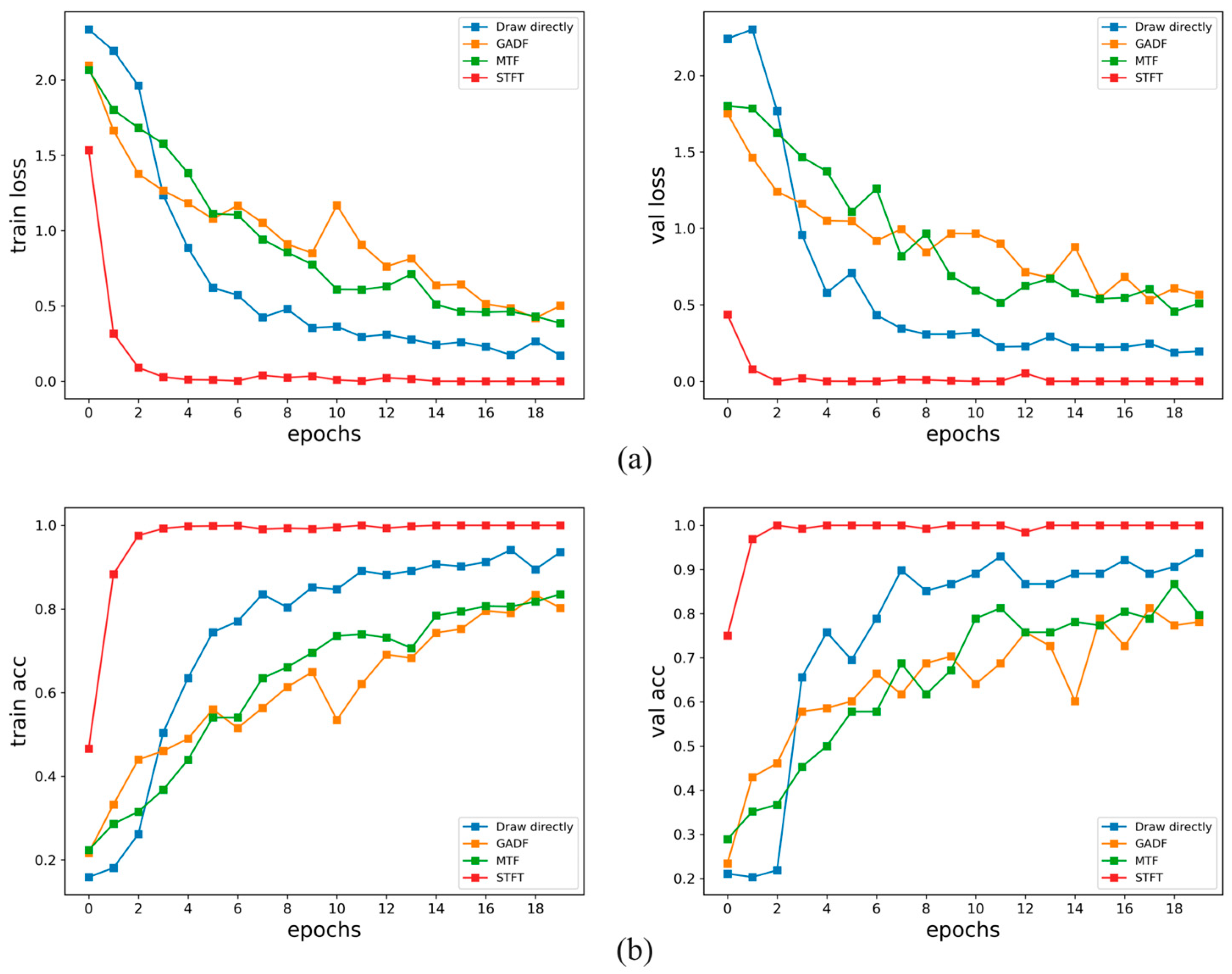
4.2.1. DE Single-Channel Data

Using a 2D spectrum map method to process bearing data of DE channel bearings under 0 HP load, the dataset was divided at ratio of 1:9, and the sample dataset was obtained as shown in

Table 2. CWRU single-channel dataset.

Label	0	1	2	3	4	5	6	7	8	9
	Normal	IR0.007	B0.007	OR0.007	IR0.014	B0.014	OR0.014	IR0.021	B0.021	OR0.021
Draw directly	244	121	123	122	122	122	122	122	122	123
	27	13	13	13	13	13	13	13	13	13
GADF	244	121	123	122	122	122	122	122	122	123
	27	13	13	13	13	13	13	13	13	13
MTF	244	121	123	122	122	122	122	122	122	123
	27	13	13	13	13	13	13	13	13	13
STFT	244	121	123	122	122	122	122	122	122	123
	27	13	13	13	13	13	13	13	13	13

. In order to verify the effectiveness of the proposed spectrum map–convolutional neural network method, Table 2 also includes three different 2D methods: the direct drawing method, the GADF method and the MTF method. Direct rendering means that bearing signals are directly converted into a 2D spectrum map using plt functions in the Matplotlib package in Python without any processing. When multichannel signals are contained, multichannel vibration signals are fused into a 2D spectrum map. The time-domain signal is encoded using the Gram angular difference field (GADF) to generate a Gram angular field image (GAF) containing the fault features. The Markov transition field (MTF) coding method uses the MTF matrix to encode the time series into a 2D spectrum map, and the 2D spectrum map corresponds to the 1D time series of the bearing vibration signal and contains the characteristics of the time series [42].

The datasets generated from four 2D methods are trained with the same VGG neural network, and the training results are shown in Figure 11 and Figure 12 and

Table 3. Final loss and accuracy of single-channel dataset in CWRU.

Method	Train Loss	Val Loss	Train Acc	Val Acc
Draw directly	0.171	0.195	0.936	0.938
GADF	0.501	0.566	0.802	0.781
MTF	0.385	0.51	0.835	0.797
STFT	0.0	0.0	1.0	1.0

. In Figure 11, the upper part is the loss function value of the training set and verification set, and the lower part is the accuracy value of the training set and verification set. Figure 11 and Table 3 show the final loss value and accuracy value after training of the dataset generated by the four 2D methods. The accuracy of the direct rendering method, GADF method, MTF method and STFT method was 93.8%, 78.1%, 79.7% and 100%, respectively, on the validation set. The vibration data processing method of STFT achieves the lowest loss value and the highest accuracy in both the training set and the verification set with a high convergence speed.

The confusion matrix and t-SNE technique were used to visualize the prediction results of the four methods, as shown in Figure 13. The error classification of the direct drawing method is mainly that 30% of 0.014 mils Ball faults are incorrectly identified as 0.014 mils outer-race faults, 50% of 0.014 mils outer-race faults are incorrectly identified as 0.007 mils ball faults and 25% of 0.021 mils ball faults are misidentified as 0.007 mils ball faults. Accordingly, misidentified categories are mixed up in the cluster graph. The error classification of the GADF method is mainly that 35% of 0.014 mils inner-race faults are incorrectly identified as 0.021 mils outer-race faults, 40% of 0.014 mils ball faults are misidentified as 0.007 mils ball faults and 0.021 mils ball faults and 80% of 0.014 mils outer-race failures are misidentified as 0.007 mils ball and 0.021 mils ball failures. Accordingly, misidentified categories are mixed up in the cluster graph. The misclassification of the MTF method is mainly that 55% of the 0.007 mils ball failures are misidentified as 0.014 mils outer-race faults and 0.021 mils ball faults, 45% of 0.014 mils ball faults are incorrectly identified as 0.007 mils ball faults and 0.021 mils ball faults, 25% of 0.014 mils outer-race failures are misidentified as 0.007 mils ball failures and 0.021 mils ball failures and 30% of 0.021 mils ball failures are incorrectly identified as 0.007 mils ball failures and 0.014 mils outer-race failures. Accordingly, misidentified categories are mixed up in the cluster graph. The STFT method obtains almost error-free obfuscation matrices and well-defined clusters.

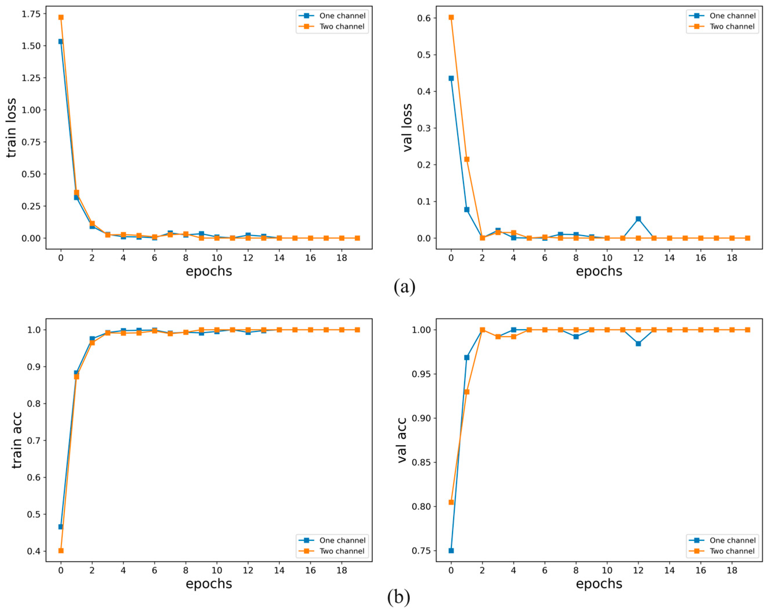
4.2.2. Dual-Channel Data of DE and FE

In the single-channel data test, the method of using the STFT to generate the spectrum map achieved good results in fault identification of the 1D vibration signal. In order to verify the effectiveness of this method in multichannel data, DE and FE dual-channel data are used to generate datasets for training. In the dual-channel experiment, three different 2D methods—the direct rendering method, GADF method and MTF method—were also used for comparison, and the number of samples was the same as that of the single channel. The training results using the dual-channel data are shown in Figure 14. In part (a) of the figure, the loss function values of the model in the training set and the validation set are shown, and part (b) shows the accuracy values of the training set and the validation set. Compared with the single-channel dataset, the accuracy of the VGG network training obtained by direct rendering method, GADF method, MTF method and STFT method was been improved, and STFT still performed best in VGG.

The training results of single-channel data and multichannel data when using STFT method are compared in Figure 15. In the training set, the influence of single-channel and dual-channel data on the fault identification accuracy is not significant, and good identification accuracy is obtained. However, in the validation set, the loss function value and accuracy of dual-channel data are more stable than that of single-channel data, which indicates that the STFT method can effectively utilize multichannel information and achieve improved fault identification accuracy in the VGG network after multichannel data processing.

4.2.3. Evaluation under Different Load Conditions

The above experiments prove that the proposed model is effective for single-channel and multichannel data under the condition of fixed power, and the multichannel data diagnosis accuracy is better. The training accuracy of data processing by STFT method is the highest. In reality, machines runs under different working conditions, so it is necessary to verify the diagnostic accuracy of the proposed method under different working conditions. 1D bearing vibration data under 1 HP, 2 HP and 3 HP loads are processed by STFT method and trained on a VGG neural network. The datasets generated under the four working conditions are shown in

Table 4. CWRU dataset of four load conditions.

Label	0	1	2	3	4	5	6	7	8	9
	Normal	IR0.007	B0.007	OR0.007	IR0.014	B0.014	OR0.014	IR0.021	B0.021	OR0.021
HP 0	244	121	123	122	122	122	122	122	122	123
	27	13	13	13	13	13	13	13	13	13
HP 1	484	122	121	123	122	122	122	122	122	122
	53	13	13	13	13	13	13	13	13	13
HP 2	484	122	122	121	122	122	122	122	122	122
	53	13	13	13	13	13	13	13	13	13
HP 3	485	123	122	123	122	122	122	122	122	122
	53	13	13	13	13	13	13	13	13	13

.

Bearing vibration datasets under four different working conditions were trained by a VGG neural network, and the training results are shown in

Table 5. Final loss and accuracy of four load conditions.

HP	Train Loss	Val Loss	Train Acc	Val Acc
HP 0	0.0	0.0	1.0	1.0
HP 1	0.002	0.057	0.999	0.994
HP 2	0.0	0.0	1.0	1.0
HP 3	0.0	0.0	1.0	1.0

, Figure 16 and Figure 17. Under four different working conditions, the accuracy of the 1 HP load is the lowest, at 99.4%. With 0 HP, 2 HP and 3 HP loads, 100% accuracy was obtained in the validation set. According to the confusion matrix and cluster graph, the bearing fault diagnosis data under four working conditions all have confusion matrices with almost no error and clusters with clear boundaries.

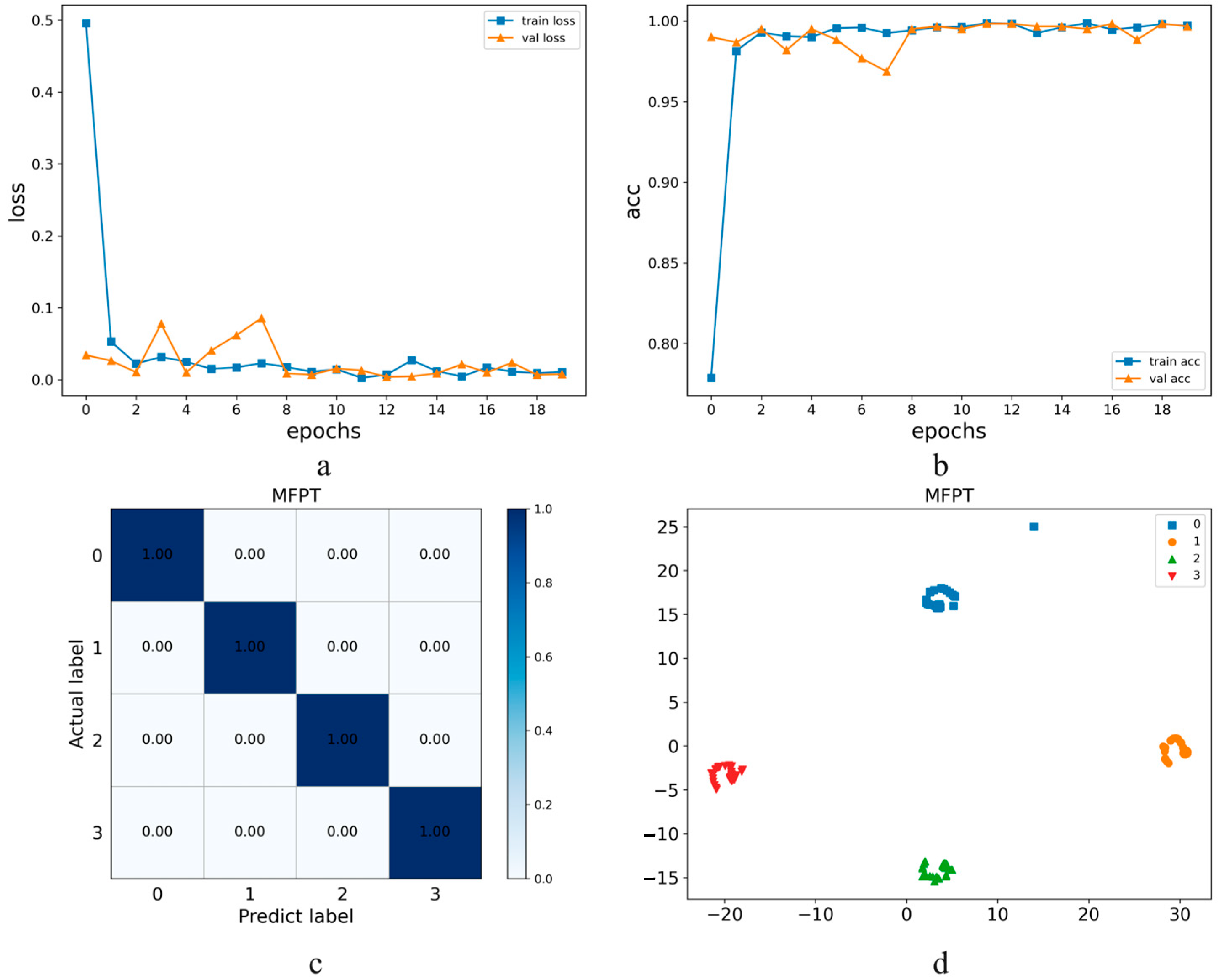
4.3. MFPT Experiment Results

The MFPT dataset was divided into four categories: baseline conditions, outer-race fault conditions, more outer-race fault conditions and inner-race fault conditions. The bearing vibration signals were converted into 2D images by STFT method. Because the MFPT dataset only contains single-channel vibration data, the generated 2D image also contains single-channel data. The dataset was divided at a ratio of 1:9, and the sample dataset was obtained as shown in

Table 6. MFPT dataset.

Label	0	1	2	3
	Baseline	Outer-Race Fault	More Outer-Race Faults	Inner-Race Fault
MFPT	1756	1757	1021	1021
	195	195	113	113

.

VGG neural network training was used for 20 epochs of training, and the training results are shown in Figure 18. A loss value of 0.011 and 99.7% accuracy were obtained on the test set, and a loss value of 0.008 and 99.8% accuracy were obtained on the verification set. According to the confusion matrix and cluster graph, four kinds of bearing faults are diagnosed by this method, and a confusion matrix with almost no errors and a cluster graph with clear boundaries are obtained. This shows that the method still has good generalization ability in different datasets and for different bearing fault diagnoses.

5. Conclusions

In the process of bearing fault diagnosis, calculation is complicated, and the accuracy needs to be improved. In this paper, a bearing fault diagnosis method based on spectrum map information fusion and convolutional neural network is proposed to realize the rapid fault diagnosis of single- and multichannel bearing signals using VGG convolutional neural networks. First, 1D bearing vibration data are processed by STFT to obtain a 2D spectrum graph. Then, datasets are divided, and a VGG neural network is used for training and diagnosis. Different channels, HP and bearings were adopted in the experiment. In dataset 1, the fault diagnosis accuracy is 100% for identification of single-channel vibration signals. Compared with common 1D data processing methods, the accuracy is the highest and the convergence speed is the fastest. When a dual-channel vibration signal is used for fault diagnosis, the two-channel model is more stable and converges faster. The lowest and highest fault diagnosis accuracies of 99.4% and 100%, respectively, are obtained in the case of 0–3 HP. In dataset 2, the parameters of vibration signals are different from those of dataset 1, and 99.8% fault diagnosis accuracy is obtained. Thus, when converting 1D time series into 2D images for fault diagnosis, the STFT transformation method can effectively represent the feature information in the signal. The VGG network structure has better classification performance for fault diagnosis. The combination of STFT data processing and VGG convolutional neural networks can make full use of multichannel data in bearing vibration signals and reduce the complex process of feature extraction so as to rapidly diagnose bearing faults in mechanical equipment with strong robustness and effectiveness. In the future work, the intelligent method will continue to be improved for bearing fault diagnosis, and the method will be applied in practical scenarios.

References

1. Shahriar, M.R.; Borghesani, P.; Tan, A. Electrical Signature Analysis-Based Detection of External Bearing Faults in Electrome-chanical Drivetrains. IEEE Trans. Ind. Electron. 2017, 65, 5941–5950. [Google Scholar] [CrossRef]
2. Li, X.; Zhang, W. Deep Learning-Based Partial Domain Adaptation Method on Intelligent Machinery Fault Diagnostics. IEEE Trans. Ind. Electron. 2021, 68, 4351–4361. [Google Scholar] [CrossRef]
3. Ma, M.; Mao, Z. Deep-Convolution-Based LSTM Network for Remaining Useful Life Prediction. IEEE Trans. Ind. Inform. 2021, 17, 1658–1667. [Google Scholar] [CrossRef]
4. Mao, W.; Feng, W.; Liu, Y.; Zhang, D.; Liang, X. A new deep auto-encoder method with fusing discriminant information for bearing fault diagnosis. Mech. Syst. Signal Process. 2020, 150, 107233. [Google Scholar] [CrossRef]
5. Cerrada, M.; Sánchez, R.-V.; Li, C.; Pacheco, F.; Cabrera, D.; de Oliveira, J.V.; Vásquez, R.E. A review on data-driven fault severity assessment in rolling bearings. Mech. Syst. Signal Process. 2018, 99, 169–196. [Google Scholar] [CrossRef]
6. Glowacz, A.; Glowacz, W.; Glowacz, Z.; Kozik, J. Early fault diagnosis of bearing and stator faults of the single-phase induction motor using acoustic signals. Measurement 2018, 113, 1–9. [Google Scholar] [CrossRef]
7. Liang, X.; Zuo, M.J.; Feng, Z. Dynamic modeling of gearbox faults: A review. Mech. Syst. Signal Process. 2018, 98, 852–876. [Google Scholar] [CrossRef]
8. Jin, Y.; Qin, C.; Huang, Y.; Liu, C. Actual bearing compound fault diagnosis based on active learning and decoupling attentional residual network. Measurement 2020, 173, 108500. [Google Scholar] [CrossRef]
9. Deng, W.; Yao, R.; Zhao, H.; Yang, X.; Li, G. A novel intelligent diagnosis method using optimal LS-SVM with improved PSO algorithm. Soft Comput. 2019, 23, 2445–2462. [Google Scholar] [CrossRef]
10. Deng, W.; Zhang, S.; Zhao, H.; Yang, X. A Novel Fault Diagnosis Method Based on Integrating Empirical Wavelet Transform and Fuzzy Entropy for Motor Bearing. IEEE Access 2018, 6, 35042–35056. [Google Scholar] [CrossRef]
11. Glowacz, A. Fault diagnosis of single-phase induction motor based on acoustic signals. Mech. Syst. Signal Process. 2018, 117, 65–80. [Google Scholar] [CrossRef]
12. Liu, H.; Zhou, J.; Zheng, Y.; Jiang, W.; Zhang, Y. Fault diagnosis of rolling bearings with recurrent neural network-based autoencoders. ISA Trans. 2018, 77, 167–178. [Google Scholar] [CrossRef] [PubMed]
13. Shao, H.D.; Jiang, H.K.; Li, X.Q.; Wu, S.P. Intelligent fault diagnosis of rolling bearing using deep wavelet auto-encoder with extreme learning machine. Knowl.-Based Syst. 2018, 140, 1–14. [Google Scholar]
14. Cheng, Y.; Lin, M.; Wu, J.; Zhu, H.; Shao, X. Intelligent fault diagnosis of rotating machinery based on continuous wavelet transform-local binary convolutional neural network. Knowl.-Based Syst. 2021, 216, 106796. [Google Scholar] [CrossRef]
15. Deng, W.; Liu, H.; Xu, J.; Zhao, H.; Song, Y. An Improved Quantum-Inspired Differential Evolution Algorithm for Deep Belief Network. IEEE Trans. Instrum. Meas. 2020, 69, 7319–7327. [Google Scholar] [CrossRef]
16. Moshrefzadeh, A.; Fasana, A. The Autogram: An effective approach for selecting the optimal demodulation band in rolling element bearings diagnosis. Mech. Syst. Signal Process. 2018, 105, 294–318. [Google Scholar] [CrossRef]
17. Qin, Y. A New Family of Model-Based Impulsive Wavelets and Their Sparse Representation for Rolling Bearing Fault Diagnosis. IEEE Trans. Ind. Electron. 2018, 65, 2716–2726. [Google Scholar] [CrossRef]
18. Shao, H.; Jiang, H.; Lin, Y.; Li, X. A novel method for intelligent fault diagnosis of rolling bearings using ensemble deep auto-encoders. Mech. Syst. Signal Process. 2018, 102, 278–297. [Google Scholar] [CrossRef]
19. Hoang, D.-T.; Kang, H.-J. A survey on Deep Learning based bearing fault diagnosis. Neurocomputing 2019, 335, 327–335. [Google Scholar] [CrossRef]
20. Jia, F.; Lei, Y.G.; Guo, L.; Lin, J.; Xing, S.B. A neural network constructed by deep learning technique and its application to intel-ligent fault diagnosis of machines. Neurocomputing 2018, 272, 619–628. [Google Scholar] [CrossRef]
21. Jia, F.; Lei, Y.; Lu, N.; Xing, S. Deep normalized convolutional neural network for imbalanced fault classification of machinery and its understanding via visualization. Mech. Syst. Signal Process. 2018, 110, 349–367. [Google Scholar] [CrossRef]
22. Lei, Y.; Yang, B.; Jiang, X.; Jia, F.; Li, N.; Nandi, A.K. Applications of machine learning to machine fault diagnosis: A review and roadmap. Mech. Syst. Signal Process. 2020, 138, 106587. [Google Scholar] [CrossRef]
23. Liu, Z.; Zhang, L. A review of failure modes, condition monitoring and fault diagnosis methods for large-scale wind turbine bearings. Measurement 2020, 149, 107002. [Google Scholar] [CrossRef]
24. Kumar, A.; Vashishtha, G.; Gandhi, C.P.; Zhou, Y.; Glowacz, A.; Xiang, J. Novel Convolutional Neural Network (NCNN) for the Diagnosis of Bearing Defects in Rotary Machinery. IEEE Trans. Instrum. Meas. 2021, 70, 1–10. [Google Scholar] [CrossRef]
25. Eren, L.; Ince, T.; Kiranyaz, S. A Generic Intelligent Bearing Fault Diagnosis System Using Compact Adaptive 1D CNN Classifier. J. Signal Process. Syst. 2019, 91, 179–189. [Google Scholar] [CrossRef]
26. Hoang, D.-T.; Kang, H.-J. Rolling element bearing fault diagnosis using convolutional neural network and vibration image. Cogn. Syst. Res. 2019, 53, 42–50. [Google Scholar] [CrossRef]
27. Guo, L.; Lei, Y.; Xing, S.; Yan, T.; Li, N. Deep Convolutional Transfer Learning Network: A New Method for Intelligent Fault Diagnosis of Machines with Unlabeled Data. IEEE Trans. Ind. Electron. 2019, 66, 7316–7325. [Google Scholar] [CrossRef]
28. Li, X.; Zhang, W.; Ding, Q. Deep learning-based remaining useful life estimation of bearings using multi-scale feature extraction. Reliab. Eng. Syst. Saf. 2019, 182, 208–218. [Google Scholar] [CrossRef]
29. Pan, J.; Zi, Y.; Chen, J.; Zhou, Z.; Wang, B. LiftingNet: A Novel Deep Learning Network with Layerwise Feature Learning from Noisy Mechanical Data for Fault Classification. IEEE Trans. Ind. Electron. 2018, 65, 4973–4982. [Google Scholar] [CrossRef]
30. Shao, H.; Jiang, H.; Zhang, H.; Duan, W.; Liang, T.; Wu, S. Rolling bearing fault feature learning using improved convolutional deep belief network with compressed sensing. Mech. Syst. Signal Process. 2018, 100, 743–765. [Google Scholar] [CrossRef]
31. Shao, H.; Jiang, H.; Zhang, H.; Liang, T. Electric Locomotive Bearing Fault Diagnosis Using a Novel Convolutional Deep Belief Network. IEEE Trans. Ind. Electron. 2018, 65, 2727–2736. [Google Scholar] [CrossRef]
32. Zhu, Z.Y.; Peng, G.L.; Chen, Y.H.; Gao, H.J. Aconvolutional neural network based on a capsule network with strong general-ization for bearing fault diagnosis. Neurocomputing 2019, 323, 62–75. [Google Scholar] [CrossRef]
33. Simonyan, K.; Zisserman, A. Very Deep Convolutional Networks for Large-Scale Image Recognition. arXiv 2014. [Google Scholar] [CrossRef]
34. Shao, H.; Xia, M.; Han, G.; Zhang, Y.; Wan, J. Intelligent Fault Diagnosis of Rotor-Bearing System Under Varying Working Conditions with Modified Transfer Convolutional Neural Network and Thermal Images. IEEE Trans. Ind. Inform. 2021, 17, 3488–3496. [Google Scholar] [CrossRef]
35. Wang, Z.; Zhao, W.; Du, W.; Li, N.; Wang, J. Data-driven fault diagnosis method based on the conversion of erosion operation signals into images and convolutional neural network. Process Saf. Environ. Prot. 2021, 149, 591–601. [Google Scholar] [CrossRef]
36. Stéphane, M. CHAPTER 4—Time Meets Frequency. In A Wavelet Tour of Signal Processing, 3rd ed.; Stéphane, M., Ed.; Academic Press: Boston, MA, USA, 2009; pp. 89–153. [Google Scholar]
37. Munteanu, M.; Rusu, C.; Vladareanu, L.; Petreus, D.; Rusu, V.; Dobra, M. EKG Analysis Using STFT Phase. In Proceedings of the International Conference on Advancements of Medicine and Health Care Through Technology, Cluj Napoca, Romania, 23–26 September 2009; p. 231. [Google Scholar]
38. Wang, X.B.; Ying, T.; Tian, W. Spectrum Representation Based on STFT. In Proceedings of the 13th International Congress on Image and Signal Processing, BioMedical Engineering and Informatics (CISP-BMEI), Electr Network, Chengdu, China, 17–19 October 2020; pp. 435–438. [Google Scholar]
39. Loparo, K. Case Western Reserve University Bearing Data Center, Bearings Vibration Data Sets; Case Western Reserve University: Cleveland, OH, USA, 2012; pp. 22–28. [Google Scholar]
40. Machinery Fault Prevention Technology Bearing Data [Online]. Available online: https://mfpt.org/fault-data-sets/ (accessed on 29 May 2022).
41. Li, M.; Zhao, Z.; Scheidegger, C. Visualizing Neural Networks with the Grand Tour. Distill 2020, 5, e25. [Google Scholar] [CrossRef]
42. Xiao, F.; Chen, Y.; Zhu, Y. GADF/GASF-HOG:feature extraction methods for hand movement classification from surface electromyography. J. Neural Eng. 2020, 17, 046016. [Google Scholar] [CrossRef]
Figure 1. VGG network structure.
Processes 10 01426 g001
Figure 2. The segmentation results of the same signal in the CWRU dataset are segmented according to the number of data points:(a) 100 points, (b) 300 points, (c) 500 points, (d) 700 points, (e) 900 points, (f) 1100 points, (g) 1300 points, (h) 1500 points and (i) 1700 points.
Processes 10 01426 g002
Figure 3. Comparison of loss function and accuracy resulting from training with different signal lengths.
Processes 10 01426 g003
Figure 4. Data segmentation.
Processes 10 01426 g004
Figure 5. The process of short-time Fourier transform.
Processes 10 01426 g005
Figure 6. The process of generating a spectrogram from the result of short-time Fourier transform.
Processes 10 01426 g006
Figure 7. Short-time Fourier transform coding: (a) divided into vibration data of a single channel, (b) divided into vibration data of two channels.
Processes 10 01426 g007
Figure 8. Flow chart of rolling bearing fault diagnosis based on a spectrum map.
Processes 10 01426 g008
Figure 9. Case Western Reserve University Rolling bearing test stand [39].
Processes 10 01426 g009
Figure 10. The generation process of the confusion matrix.
Processes 10 01426 g010
Figure 11. Training results of single-channel data in CWRU: (a) train loss and val loss; (b) train acc and val acc.
Processes 10 01426 g011
Figure 12. Final loss and accuracy of four methods.
Processes 10 01426 g012
Figure 13. Confusion matrix and cluster analysis results of four methods: (a) draw directly, (b) GAF, (c) MTF, (d) STFT.
Processes 10 01426 g013
Figure 14. Training results of dual-channel data in the CWRU dataset: (a) Train loss and val loss, (b) Train acc and val acc.
Processes 10 01426 g014
Figure 15. Training results of single-channel data and two-channel data in the CWRU dataset using the STFT method: (a) Train loss and val loss, (b) Train acc and val acc.
Processes 10 01426 g015
Figure 16. Training results of four load conditions: (a)Train loss and val loss, (b) Train acc and val acc.
Processes 10 01426 g016
Figure 17. Confusion matrix and cluster analysis results of four load conditions: (a) HP 0, (b) HP 1, (c) HP 2, (d) HP 3.
Processes 10 01426 g017
Figure 18. Diagnosis results of MFPT dataset with STFT method: (a) Train loss and val loss, (b) Train acc and val acc, (c) confusion matrix, (d) cluster analysis result.
Processes 10 01426 g018