1. Introduction
In many parts of the world, the frequency of extreme weather events has increased due to climate change. January 2019 was the hottest month on the record in Australia [
1]; the period of May–July 2007 was the wettest in 250 years and caused extensive flooding in many parts of the UK [
2]. Singapore recorded its wettest (since the record began in 1869) December in 2006 [
3]. In 2011, Thailand was struck by monsoon and tropical cyclone rains from July to October, causing extreme flooding in the city of Bangkok. More extreme climate scenarios are predicted in Australia, the UK and many other parts of the world [
4,
5,
6,
7,
8,
9].
Climate change is having an impact on the transportation infrastructure in countries like the UK [
10]. More than 160 slope failures were reported during the winter of 2000/2001 by the UK rail and road authority [
11,
12]. In many cases, meteorologically induced pore water pressure and strain softening resulting from pore water pressure cycling have been responsible for the failure of geotechnical structures [
13,
14,
15].
The changes in pore water pressure in soils are often driven by meteorological parameters, vegetation and groundwater hydrology. For more economical and sustainable design and maintenance of geotechnical structures, it is important to understand the mechanics/processes that may affect their behaviour under the current and possible future climate scenarios.
Several past fields and laboratory studies have investigated the effect of atmospheric boundaries on the behaviour of infrastructure slopes [
9,
16,
17,
18,
19,
20]. Among the numerical studies on soil-slope systems, Briggs et al. [
21], using a one-dimensional VADOSE/W [
22] model, investigated the generation of pore water pressure in a railway embankment; Tsaparas et al. [
23] modelled infiltration and compared with field observations of a sloping site in Singapore; Karthikeyan et al. [
24] presented estimation of pore water pressure using software called SEEP/W [
25] even though there was lack of agreement between the field measurements and model calculations. Rouainia et al. [
26] investigated meteorologically induced pore water pressure generation and its effect on slope stability using a coupling of SHETRAN and FLAC-TP flow and showed the capabilities of sophisticated numerical modelling approaches. However, the complexity involved in their analyses was high and needed assumptions on several modelling parameters, which can be difficult to deduce using an objective approach.
One of the more important input parameters required for analysing the interaction between soil and the atmospheric boundary is the hydraulic conductivity (
K) of soil. For a particular void ratio,
K for saturated soils (
Ksat) can be treated as a constant. However, the same does not apply to the case of
K for unsaturated soils (
Kunsat). It changes with soil suction even if the void ratio remains the same. The soil suction, on the other hand, is dependent on the soil’s degree of saturation. Direct measurement of
K will involve measurement of water flow. However, as soon as some flow has occurred, the water content will change, which will lead to a change in suction and eventually the
Kunsat. Due to this, it is extremely difficult to measure
Kunsat for soils. Several methods have been proposed in the literature to capture the suction-
Kunsat correlation [
27,
28,
29] and commonly,
Kunsat is expressed as a function of
Ksat and soil suction. For example, Van-Genuchten [
27] proposed the following equation,
where
,
n and
m are curve fitting parameters and
Ψ is the matric suction. In essence, with a reasonable estimation of the soil–water characteristics curve (SWCC) and
Ksat, Equation (1) can be used to estimate the
Kunsat.
A challenge in using Equation (1), often overlooked, is the estimation of
Ksat. Several field tests (e.g., single or double ring infiltrometer, disc permeameter, Guelph permeameter, bailout test) and laboratory tests (e.g., Rowe cell, constant/falling head tests, Oedometer tests, triaxial hydraulic conductivity tests) have been developed and routinely conducted to deduce
Ksat. However,
Ksat deduced from a different field or laboratory tests can be very different, which is partly due to the underlying assumptions involved in those methods. Discrepancies of several orders of magnitude are not uncommon [
9]. The field tests are often believed to yield more representative
Ksat values compared to the laboratory tests. However,
Ksat values deduced from field tests can also be affected by the presence of hidden cracks or fissures in the soil, local heterogeneity and the presence of higher hydraulic conductivity layers, which may not be detected during the field investigation. Thus, the conventional methods of deducing
Ksat can have a low degree of reliability. For example, in the study site involved in this investigation (discussed in the next section), more than 100 times difference in
Ksat values from different tests were observed. This makes it very difficult, and in some cases, impossible to objectively decide what value of
Ksat to be used in a particular analysis [
30]. The engineer is often forced to use either an average value or make a subjective judgement which can be influenced by the engineer’s experience with similar sites or the lack of it. For a seepage analysis involving unsaturated soil, the problem becomes even more complex due to the dependency of
Kunsat on the soil’s degree of saturation.
This paper discusses a simple and objective approach for estimating
Kunsat using a correlation similar to one presented in Eq. [
1]. The method involves a systematic back-analysis of field observations to deduce
Kunsat as a function of
Ksat. The method of estimation of
Ksat was originally proposed by Lo et al. [
31] to estimate
Ksat for prefabricated vertical drain improved soils.
Ksat, in their case, was estimated by systematically analysing field settlement data. It allowed them to avoid explicit modelling of the smear zone and reduced
Ksat due to smearing in that area which is often very difficult to determine due to limited time and budget associated with field investigation of a practical project. The effectiveness of the method in different problem domains has been demonstrated in the literature by Karim [
32], Karim et al. [
33], Manivannan et al. [
34], Karim et al. [
35] and Lo et al. [
36]. The approach has been modified in this paper for analyses in the unsaturated domain, i.e., to estimate
Kunsat. The effectiveness of the method has been put to the test by modelling a well-instrumented research site located in Southern England [
20]. A selected period of monitoring data (from 1 January 2006 to 31 December 2008—a total of 3 years) have been used. A finite element software SEEP/W (version 2021.4) [
37] has been used for this purpose.
In the next section, the research site is discussed in terms of its construction, geotechnical properties, instrumentation and monitoring details. Different aspects of the numerical analyses, including the mesh or geometry chosen, boundary conditions and other input parameters, are discussed in the next section. Subsequent sections discuss the results and conclusions drawn from this paper.
2. Newbury Cutting—The Research Site
The research site discussed in this paper, hereafter referred to as Newbury cutting, is located near A34 Newbury bypass in Southern England. The location of the site is presented in
Figure 1. The site was extensively instrumented and monitored. Details of the site instrumentation, monitoring, geology and weather data can be found in Smethurst et al. [
20] and Smethurst et al. [
19]. For the sake of completeness, a brief description is presented here.
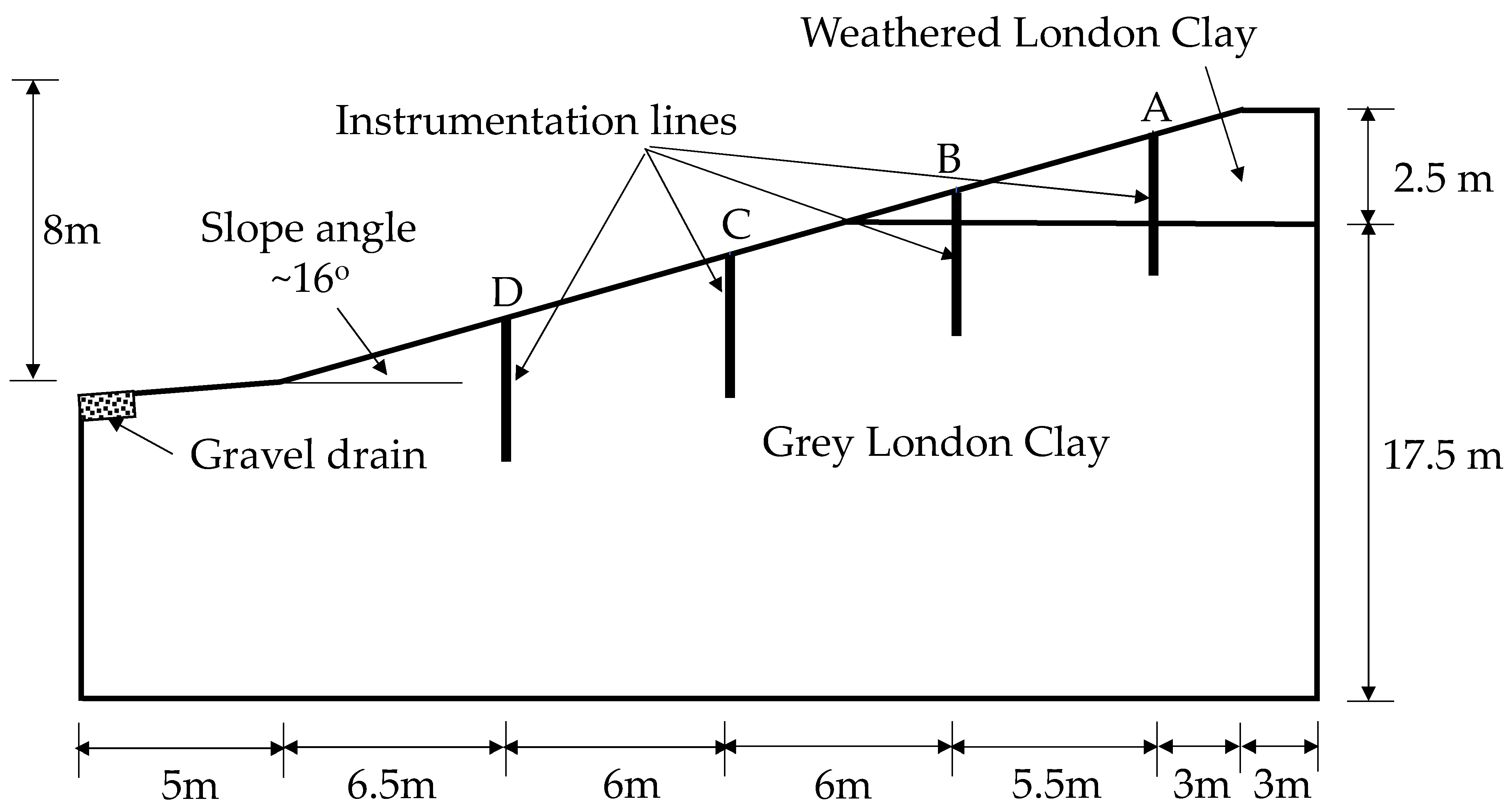
The instrumented section of the cut slope was 8 m high and 28 m in length along the sloping direction, as presented in
Figure 2. The slope was excavated in 1997. The site soil consists of stiff grey London clay of about 20 m thickness and its properties have been found to vary in the vertical and horizontal directions. The top 2.5 m of the slope, below the original ground level, was extensively weathered and hereafter referred to as weathered London clay. The presence of several bands of silty clay up to 50 mm thick and large flints was also detected during the site investigation. After the cutting was excavated, a 0.4 m layer of topsoil was placed over the cut surface to facilitate the planting of vegetation. To facilitate quick drainage, a fin drain was also installed near the toe of the slope.
A series of field and laboratory tests were conducted by Smethurst et al. [
20] to deduce different soil parameters for the research site. The tests included Atterberg limit tests, triaxial (saturated) hydraulic conductivity test, dry unit weight test and field saturated hydraulic conductivity test using the bail-out method. The deduced
Ksat, unit weight, and plasticity indices of the site soil are summarised in
Table 1. It is to be noted that a large number of laboratory tests on undisturbed samples along with bailout tests (in the field from hand augured boreholes of up to 3 m deep) were used to deduce the
Ksat values. 1 to 3 orders of magnitude differences between deduced
Ksat values were reported by Smethurst et al. [
20]. It was believed to be due to anisotropy and soil fabric, including silt partings and cracks and fissures.
The relationship between the soil water content and suction (also known as soil water characteristics curve—SWCC) for London clay was reported by Croney [
39] and is presented in
Figure 3 and can be assumed to be representative of the site soil [
9]. It is to be noted that Croney [
39] presented SWCC for both drying and wetting stages for London clay. As SEEP/W [
37] does not allow the use of multiple SWCCs and also considering the difficulties associated with generating consistent wetting SWCC, the drying curve was used for this analysis. It is expected that if the wetting SWCC was used, the observed pore water pressure response would be different as
Kunsat is a function of
Ksat and SWCC. Change in one may require adjustment in the other parameter. However, its significance was outside the scope of this study.
Moreover, it should be noted that SEEP/W [
37] and most other numerical software use SWCC in terms of volumetric water content and the curves presented by Croney [
39] were in terms of gravimetric water content. The gravimetric values were converted into volumetric values using the following relationship (Equation (2)) and the transformed SWCCs are presented in
Figure 3.
where
wvol is the volumetric water content,
wgr is the gravimetric water content, γ
dry and γ
w are the dry unit weight of soil and unit weight of water, respectively. The average values for γ
dry for the two different soil layers were used for the calculations, as presented in
Table 1.
The vegetation on the slope was predominantly rough grass and herbs with some small shrubs (0.5 m < tall). The grass and herbs were mowed periodically until October 2002 to help the development of shrubs planted on the slope. Several grown-up Beech, Oak and Silver birch trees were located near the top of the slope.
Instrumentation was done to monitor moisture content (TDR moisture probes), suction (standard water-filled tensiometers and equitensiometer), positive water pressure (piezometers), and water table location (dipping boreholes) at depths between 0.3 and 3.5 m. The instruments were installed in four groups, namely, cluster A (near the crest) to D (near the toe). A weather station was also installed at the site. A 350 mm deep interceptor drain was installed on the slope face (across the slope face) to capture surface runoff and interflow. The site was monitored from October 2002.
Figure 4 and
Figure 5 present average daily rainfall and runoff recorded (respectively) for the 3 years duration under consideration in this study. Other recorded meteorological parameters for the duration, i.e., average daily temperature, average daily wind speed (2 m above ground surface) and average daily humidity, are presented in
Appendix A. These data will later be used in calculations.
3. Numerical Analyses
SEEP/W [
37] is a finite element software that allows analysis of groundwater seepage and pore water pressure distribution within porous media such as soil in both saturated and unsaturated states. The types of analyses can range from saturated steady-state problems to complex saturated/unsaturated time-dependent (transient) problems. The pore water pressure distribution from such analyses could be used as an input for other stress or stability analyses to assess the serviceability and ultimate limit state behaviour of the slopes.
The software requires SWCC and soil hydraulic conductivity function (i.e., variation of K with soil suction) as inputs for material definition. The effect of climate variables on the problem can be modelled using an equivalent hydrological boundary condition (explained later). Different modelling aspects of the problem are discussed in the next few sections.
3.1. Model Geometry
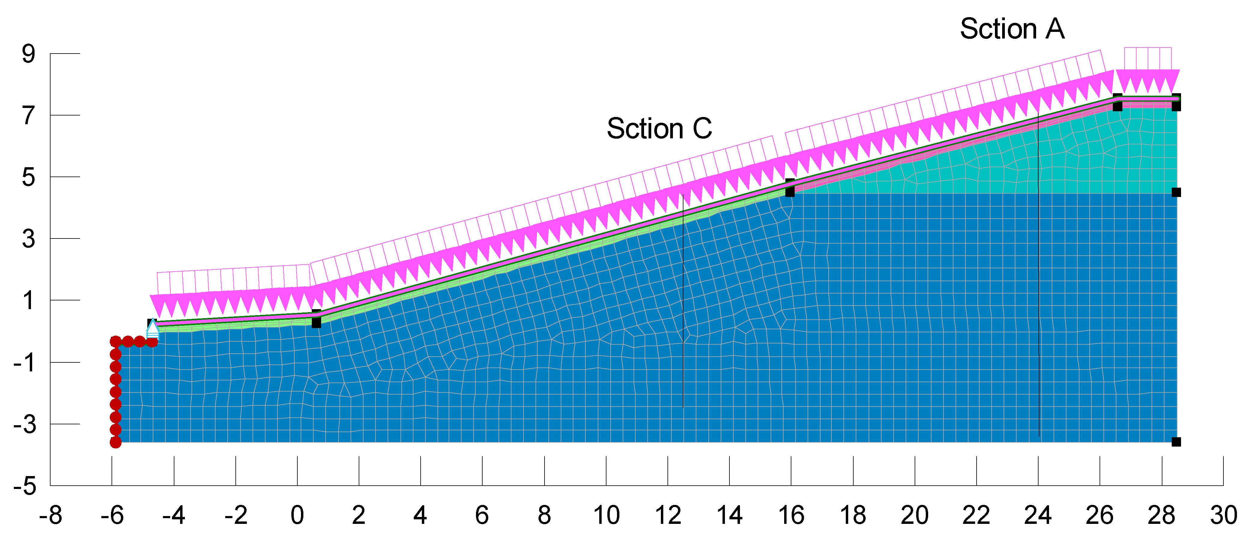
The discretised geometry used for the analysis is presented in
Figure 6. To minimise the effect of imposed boundary conditions on the analysis results, the geometry was extended by 20 m towards the right and by 15 m towards the left. Several trials were run to ensure the effect of boundary and mesh size was minimum or insignificant to the observed results. Details of the trials are presented in
Appendix B. A global mesh size of 0.8 m was used in the analysis. Except for the surface layer, the geometry was discretised using an automatically generated unstructured mesh using triangular and quadrilateral elements. The elements close to the boundary (to a depth greater than the maximum depth of measurement during field investigation) were then refined to half the global element size. The surface layer was discretised using quadrilateral elements. Quadrilateral elements have been shown to perform better in such scenarios as the gradients of primary unknowns are steeper in the direction normal to the surface [
37]. The nodal convergence was checked. A total of 4200 nodes and 3965 elements (4-nodded quadrilateral and 3-nodded triangular) were used to discretise the geometry.
The soil in the slope had two distinct subdivisions, namely, weathered London clay and grey London clay layers. They were modelled using different materials. Because of the presence of plant roots and other organic matters, the K of the top surface of the soil slope was higher than the layers below. Separate surface layers (of 0.4 m thickness with element thickness of 0.1 m) using different material models were added to the geometry to account for these differences (i.e., surface layers corresponding to weathered London clay and grey London clay layers). The pore water pressure and other variables usually change rapidly close to the exposed soil surface, i.e., in the surface layer.
3.2. Material Models
SEEP/W [
37] allows the soil to be modelled as saturated only or as a combination of saturated and unsaturated soil states. All four soil materials (i.e., grey and weathered London clay and their respective surface layers) were modelled using the saturated/unsaturated option. This way, the soil could stay in a saturated or unsaturated state during an analysis or change state depending on the analyses conditions. The SWCCs for the weathered and grey London clay have been discussed above. The SWCC for the surface layers was kept similar to the layers below. There were no specific
K data available for the surface layers. The
Ksat values for the soils were assumed as 10 times the values of the layers below [
40].
3.3. Calculation for Input Hydrological Boundary Condition
The water balance equation [
41] was used for the calculation of input hydrological boundary conditions to represent the effect of the atmospheric boundary (e.g., rainfall, solar radiation, humidity, wind speed) and vegetation as below,
where
R is the rainfall,
RO is the runoff,
ET is the evapotranspiration,
S is the change in stored water within the soil, and
RE is the net recharge from surrounding soils. If we consider inflow and outflow for soil mass from the surrounding soil is equal, i.e.,
RE = 0, we can say
S is equal to the magnitude of water percolating into the soil, net surface infiltration (
NSF) through the surface boundary. Thus we can rewrite Equation (3) as below,
The measured daily rainfall and runoff and calculated
ET data were used for this purpose. To estimate
ET, a reference
ET was calculated first using the Penman-Monteith equation as below [
42],
where
ETr is the reference evapotranspiration calculated in a 1-day time step, Δ is the slope of saturation vapour curve,
Rn is the net radiation flux in MJ/m
2/day,
G is the soil heat flux density in MJ/m
2/day,
γ is the Psychrometric constant in kPa/°C,
T is the mean temperature in °C 2 m above the ground level,
u2 is the wind speed in m/s at 2 m above the ground, and (
es −
ea) is the saturation vapour pressure deficit in kPa.
The Penman–Monteith equation [
42] parameters presented in
Table 2, along with the weather data presented in
Appendix A have been used. Once the daily
ETr was calculated,
ET was deduced using the following equation,
where
SMD is the soil moisture deficit,
RAW is readily available water, and
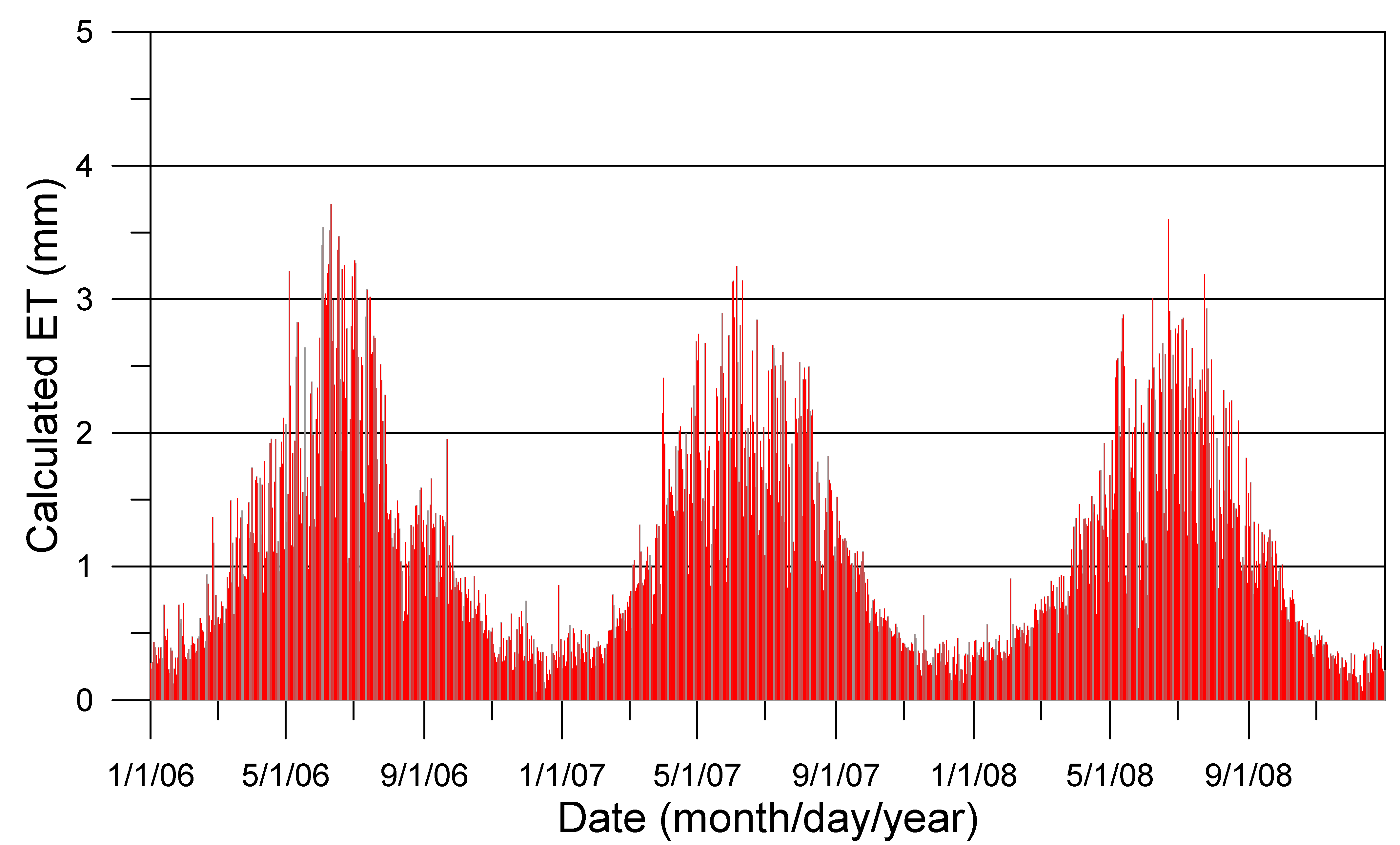
TAW is the total available water. Calculated
ET values are presented in
Figure 7 and calculated daily
NSF values are presented in
Figure 8.
NSF values represent the infiltration of water into the soil due to rainfall and also the removal of water due to evapotranspiration.
NSF can be of either positive or negative magnitude. A positive value will indicate water is infiltrating into the ground and the rainfall is dominating the process. A negative value, on the other hand, will indicate water is leaving the soil due to evapotranspiration. The calculated
NSF values were used as an input hydrological boundary condition for this analysis and represented the effect of climate and vegetation on the problem. It is to be noted that while using eq [
3] to estimate
NSF, the value of runoff needs to be known. However, it may not be a readily available measurement. In the absence of measured runoff values, a process outlined in
Appendix C can be used to estimate runoff and thus
NSF. Similar approaches have been used in the literature [
9,
43,
44].
It is to be noted that the use of a 1-day time step means everything occurring within a particular 24 h period is averaged out over that period and the effect of a shorter duration event may not be captured very accurately. It is possible to conduct a similar analysis with smaller time steps (e.g., hourly) if hourly measurements of all related parameters were available.
3.4. Other Boundary Conditions
The left, right and the bottom boundary of the problem was modelled as impermeable (no flow). Part of the ground surface with road surfacing was modelled as impermeable as well. The mesh and geometry sensitivity analyses show that the choice of these boundary conditions was appropriate. The fin drain installed near the toe of the slope was not modelled explicitly. Rather its effect was modelled using a zero pore water pressure boundary. A flux boundary condition was applied at the ground surface, as discussed earlier.
3.5. Initial Condition
The initial pore water pressure condition in the model was established using an initial water table. An educated guess was made by analysing the piezometer pore water pressure data on the date 1 January 2006. This might have some effect on the predicted pore water pressure profile, and to the author’s understanding, a more complicated seepage analysis could be conducted to establish the initial pore water pressure profile. However, as will be shown later, the effect of assuming an initial water table gets diminished as the analysis progresses and somewhat becomes irrelevant beyond a few months of analysis, even when a very crude guess is made.
3.6. Estimation of K
For modelling unsaturated soils, SEEP/W [
37] allows the choice of different functions that deduces
Kunsat by relating soil suction to
Ksat. A user can choose from available functions such as Fredlund et al. [
29], Green and Corey [
28] and Van-Genuchten [
27]. In this investigation, the Van-Genuchten [
27] function (Equation (1)) was used. Estimating an appropriate value for
Ksat was a challenge as large (more than 100 times) differences were observed for values from different tests. As indicated earlier, in such scenarios, one has a choice of using an average value or using subjective judgment.
An alternative approach was used to estimate a representative
Ksat value in this study. The first year of field-measured pore water pressure data was back analysed. Few trial analyses were conducted with
Ksat being systematically varied until the best match was found. The field average
Ksat as presented in
Table 1, was used as the first trial value. SWCC and other parameters in the study remained unchanged (e.g., the ratio between
Ksat in surface layers and the underlying layers). The best match
Ksat values were then used to analyse the problem further. Piezometer readings from two different depths at two locations, A and C (see
Figure 2 and
Figure 6), were used.
In principle, this process is not very different from conventional techniques (especially field tests) used to deduce Ksat. Interpretation of many of the field tests also involves several assumptions and back-fitting of field observations. For example, in a Guelph permeameter test, the flow of water into the soil is observed, and collected data are interpreted using saturated-unsaturated flow theories to estimate Ksat.
Figure 9 presents the effect of using different
K values on the pore water pressure profile for location C at 2.5 m depth. Three different analyses are presented here, i.e., analysis using the field average
Ksat, analysis using the best match
Ksat and analysis using three times the best match
Ksat. The figures show that
Ksat may play a significant role in such pore water pressure analyses. The best match
Ksat values for the weathered London clay and grey London clay were 0.015 m/d and 0.0025 m/d, respectively—approximately four and eight times their respective field average values. Plots at other locations are not presented here due to space limitations.
4. Results
The analyses were run from 1 Jan 2006 to 31 December 2008, a total duration of 3 years, including the first year used for the estimation of Ksat. The results are discussed below.
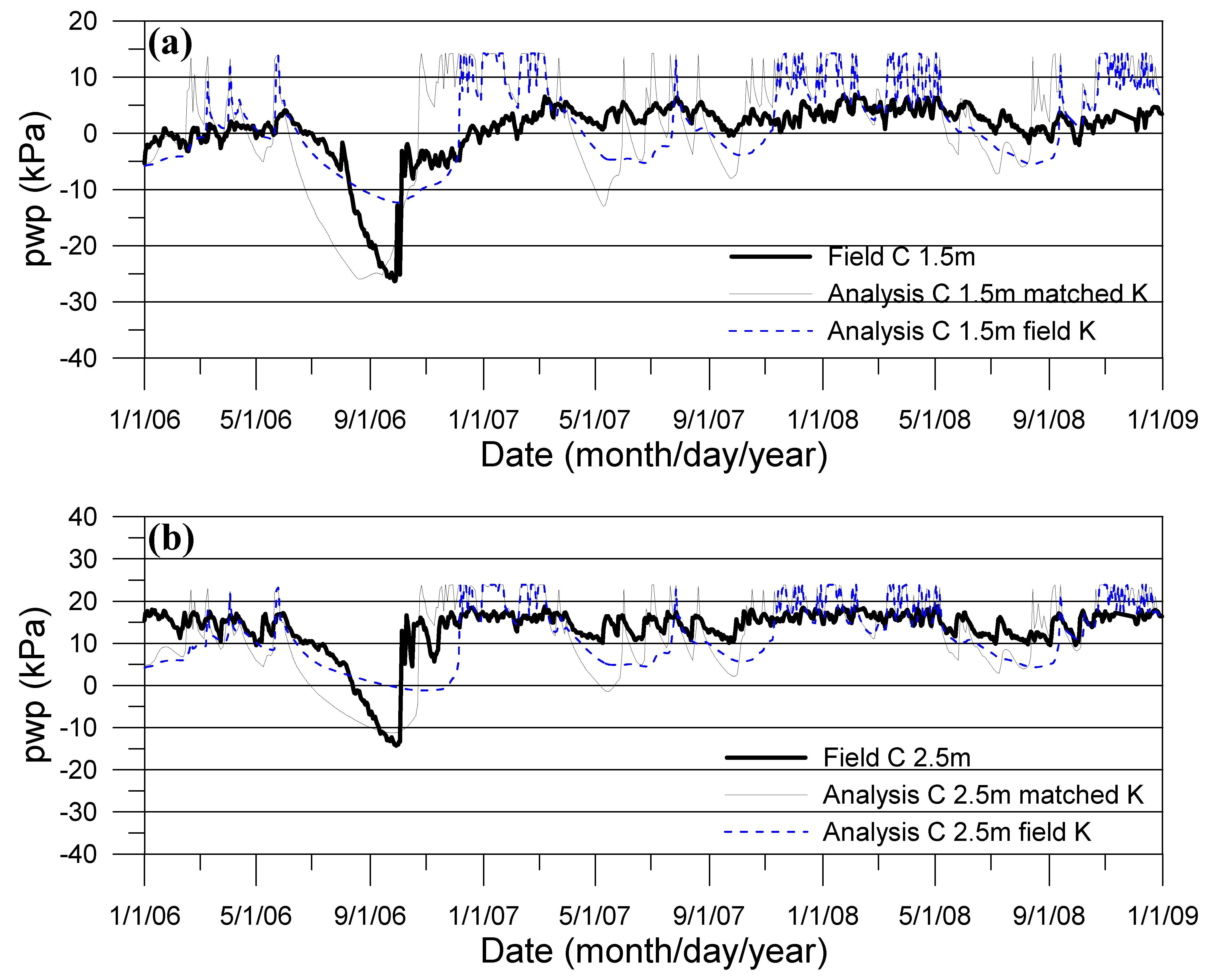
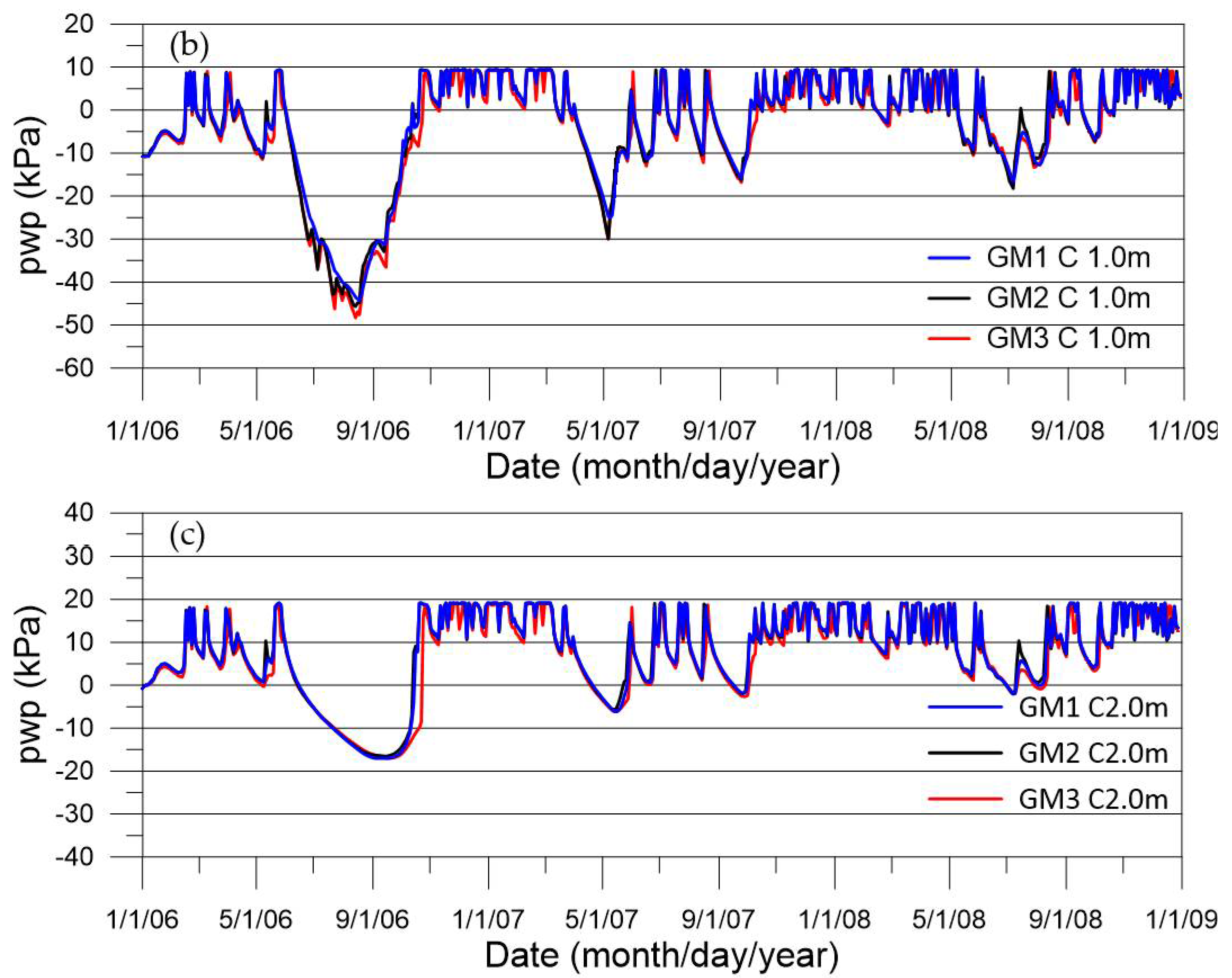
Figure 10a,b show the field measured and calculated pore water pressure from two analyses (i.e., one using matched
K and the other using average field value) at 1.5 and 2.5 m depths from the surface at instrumented section A and
Figure 11a,b presents the same for location C. At location A, both analyses captured the negative pore-water pressure peaks with reasonable accuracy. Both analyses (using matched and field
K) overestimated the magnitude of positive pore water pressure throughout the measurement period. At location C, the qualitative trend (peaks and troughs) was much better captured in the matched
K analysis and the use of average field
K in the analyses led to a significant underestimation of negative pore water pressure developed during the period of June-July of 2006. The number of peaks and troughs in the field measured values were better captured by using matched
K in the analyses. The average
K analysis trend was relatively smoother and often did not capture the smaller peaks and troughs in the trend (short duration events). Overall, the use of matched
K improves the accuracy of the calculation.
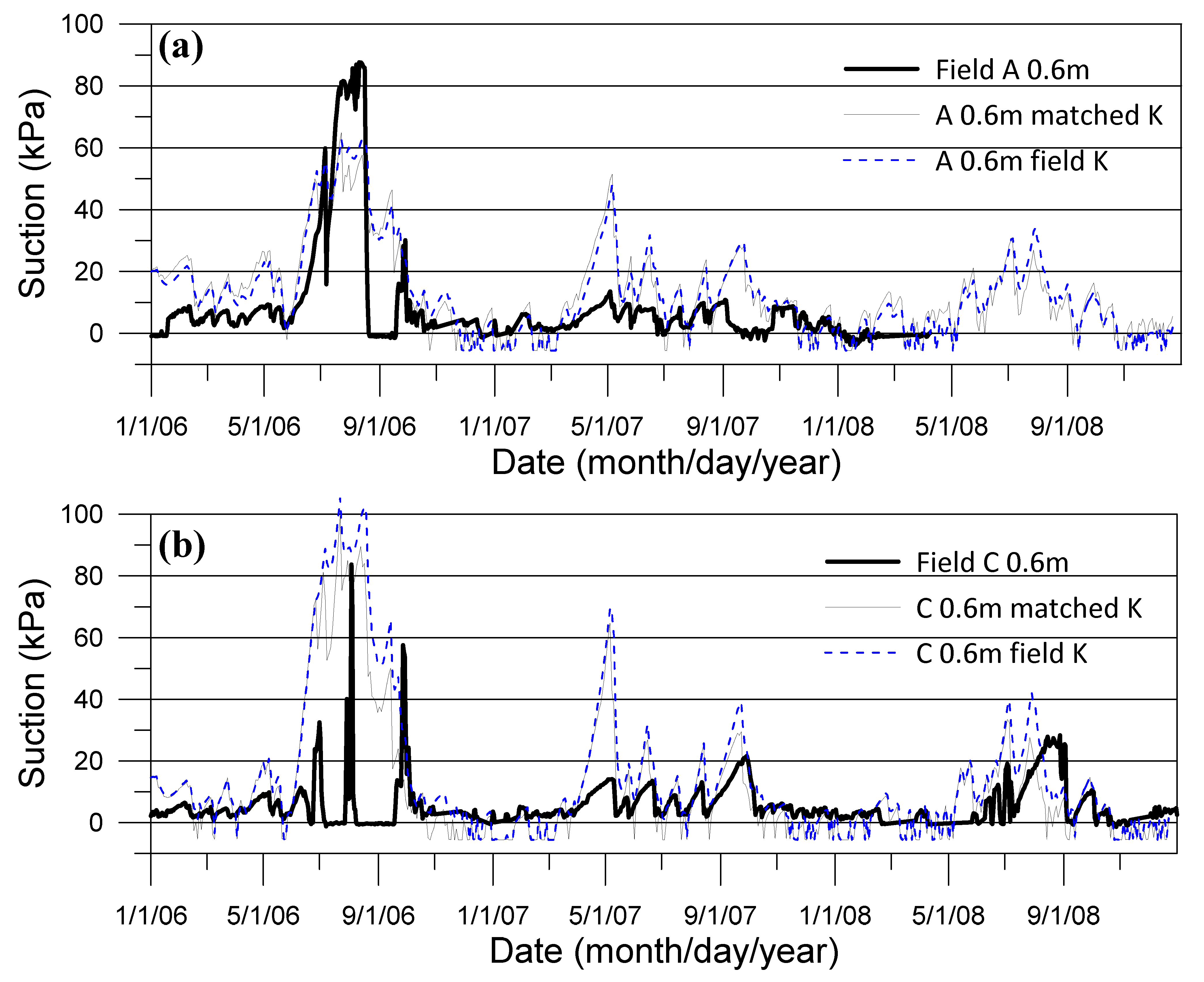
The near-surface soil suctions were recorded by standard water-filled tensiometers at different depths (0.3, 0.6 and 0.9 m from the surface at locations A and C).
Figure 12a,b present the measured suction and estimated responses from the numerical analyses (both using field average
K and matched
K) at 0.6 m depth at instrumented locations A and C, respectively. At location A the suction magnitude was underestimated between June and July 2007 and overestimated at other times by both analyses. The difference between the calculations from the two analyses was very small. At location C, the suction response was significantly overestimated by both analyses. The overestimation was slightly higher for the case of the field
K analysis. The qualitative trend was reasonably well captured by both analyses with reasonable accuracy.
Figure 13 presents the measured and calculated volumetric water content variation with time. At location C, both analyses calculated volumetric water content with reasonable accuracy; however, at location A, both analyses significantly underestimated the changes in water content with time. This difference is likely to be due to local heterogeneity of the soil and the SWCC used in the analyses is unable to represent its behaviour. It is to be noted that in a saturated/unsaturated seepage analysis, the hydraulic conductivity and SWCC both affect the changes in water content (as
Kunsat is a function of soil suction) and consequently developed pore water pressure. Estimating the
Kunsat based on observation of pore water pressure response has allowed prediction of the same with greater accuracy. It is to be noted that the estimation of
Kunsat could also be achieved by comparing the predicted and field observed water content data, and in such a case, it is expected that the prediction of water content could have improved accuracy. It is envisaged that with a better estimation of SWCC for different materials used in the simulation, a better estimation of water content could be achieved.
The interaction between soil, vegetation and the atmospheric boundary is complex and can be influenced by a number of variables. This paper presents a simplified process to model the interaction to capture the related changes in water pressure and soil water content and outlines an objective approach to estimate one of the most important parameters in seepage analyses (i.e., hydraulic conductivity). The simplification and assumptions include,
the use of an SWCC from literature for a similar soil (not based on soil tested on this particular site)
the use of the drying curve for representing both wetting and drying behaviour
the assumption of uniform soil properties within different soil layers even though the site investigation revealed the grey London clay to be variable along with the vertical and horizontal directions.
Despite these simplifications, the analyses presented here could capture the qualitative trend and quantitative changes in pore water pressure and water content with reasonable accuracy. The difference between the field averaged value of Ksat and matched Ksat was four to eight times. It is to be noted that standard laboratory or field tests for hydraulic conductivity often produce estimates that can be 100 or even 1000 times different from each other. Furthermore, the calculation here was found to be significantly less sensitive to Ksat compared to seepage or consolidation analyses in saturated soils. Due to this, the differences between the field average K analysis and matched K analysis were close to each other on many occasions, even though the matched K analysis showed a relatively better overall prediction for water pressure and water content. In other situations where more variability exists, the situation may be significantly different, and the use of field average K may produce far inferior predictions.


