Article

Simulation of Fracture Morphology during Sequential Fracturing

1
College of Geology and Environment, Xi’an University of Science and Technology, Xi’an 710054, China
2
College of Petroleum Engineering, Xi’an Shiyou University, Xi’an 710065, China
3
Research Institute of Petroleum Exploration and Development, Liaohe Oilfield Company of Petro, Panjin 124000, China
4
Gas Production Plant 2 of Yanchang Gasfield, Shaanxi Yanchang Petroleum (Group) Co., Ltd., Jingbian 718500, China
5
No. 11 Oil Production Plant of Petro-China Changqing Oil Field Company Ltd., Xi’an 745400, China
*
Authors to whom correspondence should be addressed.
Processes 2022, 10(5), 937; https://doi.org/10.3390/pr10050937
Submission received: 20 April 2022 / Revised: 5 May 2022 / Accepted: 6 May 2022 / Published: 9 May 2022

Abstract

:
During hydraulic fracturing, the aperture of hydraulic fractures will shrink by the in-situ stress, but will not fully close because of the existence of proppant inside the fracture. In previous studies, few people noticed the existence of proppant, which has resulted in the inaccuracy of simulation results. In this study, based on the boundary element method, a numerical simulation model for sequential fracturing was established, which respectively considered the influence of proppant in staged fracturing and zipper fracturing. In addition, the influence mechanism of proppant on fracture morphology is then revealed. Simulation results show that the residual aperture of the previous hydraulic fracture, which was produced by proppant, may increase with the increase of proppant stiffness and fracture spacing and may also be shrunk by the dynamic propagation of subsequent hydraulic fracture. However, the residual aperture will rebound after hydraulic fracturing construction is finished. The shrinkage and rebound values of residual aperture of hydraulic fracture are usually less than 1 mm. In addition, at the same time, the residual aperture of previous hydraulic fracture may also influence the propagation of subsequent hydraulic fracture. These influences are represented by the bend of fractures in multistage fracturing and the intersection in zipper fracturing. With the increase of well spacing, the influence degree of residual aperture on subsequent fracture propagation is reduced. The previous hydraulic fracture cannot have a significant effect on the deflection of subsequent hydraulic fracture when fracture spacing is between 10 and 30 m. The above research has important guiding significance for controlling fracture morphology in hydraulic fracturing.

1. Introduction

Unconventional oil and gas resources are important components of traditional fossil fuels [1]. Studies have shown that human consumption of oil and natural gas remains dominant. However, due to the low permeability and porosity of the unconventional reservoir, it cannot achieve economic productivity without technological measures of increasing recovery efficiency. Waterflooding is one of these methods. However, waterflooding has the problem of salt precipitation and permeability reduction. Salt precipitation may result in permeability reduction during waterflooding under high pressure and high-temperature conditions [2,3] in addition to permeability reduction due to asphaltene precipitation in the near-wellbore region of oil wells [4]. In order to reduce the production costs and improve the recovery efficiency of oil and gas, various fracturing techniques have been proposed, like the horizontal well staged fracturing technology [5], zipper fracturing technology [6], synchronous fracturing technology [7], refracturing technology [8], etc. The common point of the above technologies is that multiple fractures propagate sequentially and interfere with each other. Especially in recent years, with the proposal of close cutting fracturing technology and infill wells conception, the interference situation between fracturing wells and hydraulic fractures (HFs) has received obsessive attention [9,10]. Revealing the disturbance between HFs and fracturing wells can help to improve the effectiveness of reservoir fracturing, ultimately enhancing oil and gas recovery [11]. Therefore, it is necessary to study the effects of multi-fracture interactions on fracture trajectories and deformation.
Due to the limitation of sample size, it is different to display the mutual interference during fracture propagation in physical experiments. Thus, numerical simulation technology is an important way to study this scientific problem. Zheng [12] simulated the well interference on hydraulic fracture propagation during zipper fracturing, proposing that asymmetric fracture propagations occur in multi-well fracturing, and the lateral growths of interior fractures are suppressed due to the intense inter-well stress interference. Guo [13] investigated the effect of six factors on the fracture propagation. These factors include plasticity and brittleness, horizontal stress difference, cluster spacing, fracturing fluid viscosity, pumping rate, and cracking sequence. The results showed that, in simultaneous fracturing, the fracture network is formed spontaneously. With the same brittleness of the reservoir, fracture in zipper fracturing always propagates slightly longer than that in simultaneous fracturing. The results provide theoretical support for both zipper and synchronous fracturing modes, which helps design well completion and fracturing operation parameters. Zheng [14,15] proposed simulation of the propagation of multiple closely spaced fractures, and simulation results show that closely spaced perforation clusters in a stage tend to be unevenly and asymmetrically initiated, and a coalesce situation likely occurs when fracture space is too small. Zhang [16] verified this mechanism by a physical experiment. In multiple vertical wells, 3D fractured areas produced in simultaneous fracturing are much smaller than those produced in sequential fracturing [17]. Saberhosseini [18] used an extended finite-element model by ABAQUS to study the multiple fracture growth in modified zipper fracturing, proposing that we should pay attention to the flow rates and the injection to prevent multiple hydraulic fracture deviation and collision. Zhou [6] simulated the periodic variation law of induced stress in modified zipper fracturing, and proposed that arranging a perforating position through fracturing units can effectively increase the reservoir reconstruction area. In addition, at the same time, Sukumar [19] quantified the degree of pressure communication between adjacent reservoirs based on field data for the first time. Some three-dimensional and fully coupled models were proposed to study the interaction between multi-fractures [20,21,22].
However, in numerical simulation, the interference model between closed fracture and dynamic propagation fracture still has some deficiency. Whether in simultaneous or sequential fracturing simulation, the reverse support of proppant on compression fractures is often ignored [15,23,24,25]. Based on the boundary element method, Li [26] proposed nonlinear normal stiffness and studied the propagation of rock joint under compression. However, the rock joint model was proposed based on a natural fracture; it is not suitable for HFs. In general, hydraulic fractures are supported by two forces during fracturing: pressure from the injected fluid and reactive force from proppant. The above rock joint model did not consider the initial aperture of HF caused by hydraulic fracturing. Cheng [27] studied the simultaneous and sequential fracturing while considering the nonlinear closure of the fracture. However, in his simulation model, the shrinkage of HF aperture is calculated on the basis of the contraction in the previous step, which cannot reflect the superposition of proppant counterforce. In this paper, a mathematical model is established, taking the comprehensive change of the fracture aperture as unknown in order to reflect the superposition effect of the counter-support force. In addition to this, there are still some fracture interaction mechanisms that have not been revealed, such as fracture morphology when normal stiffness is considered in zipper fracturing.
In conclusion, the aim of this paper is to establish a multi-fracture propagation interaction model considering fracture plane support and study the interaction mechanism between hydraulic fractures. The rest of this paper is organized into the following four sections. Section 2 is the construction of the computational model and relevant validation. Numerical simulation analysis and discussions are presented in Section 3 to study the aperture and trajectory of HFs, the induced stress distribution situation. Section 4 presents some conclusions.

2. Numerical Model

2.1. Model Assumption

In reality, the propagation of hydraulic fracture is the combined effect of multiple physical fields. At present, it is difficult to establish a simulation model coupling all physical fields. Thus, in order to simplify the calculation model, and focus our research on fracture morphology and stress interference in the horizontal well, the following assumptions are introduced to establish the numerical model: (1) Isothermal conditions, the influence of temperature on fracture deformation during fracture propagation is ignored; (2) The model is homogeneous and isotropic, that is, do not consider the heterogeneity of rock mechanical properties and abnormal pressure caused by geological tectonic movement; (3) The target formation belongs to linearly elastic medium, that is, the load and deformation obey Hooke’s law [28]; (4) Fracture belongs to the KGD model, that is, HF is a vertical fracture with constant height, and the horizontal plane satisfies the plane strain condition for a short fracture relative to height [29]; (5) The study domain is infinite and ignores the abnormal pressure caused by geological tectonic movement; (6) The fracture propagation process follows the theory of linear elastic fracture mechanics [30], that is, the linear theory of elasticity is used to analyze the crack, and some characteristic parameters, like stress intensity factor, are used to judge the crack growth; (7) The fluid within the fracture is incompressible and belongs to the Poiseuille flow between two parallel plates [31].

2.2. Discontinuous Displacement Method

The displacement discontinuity method (DDM) is one of the boundary element methods (BEM) and was first proposed by Crouch [32]. In this paper, we use DDM to simulate the deformation of fracture and induced stress field. Separate HF into N segments of discontinuous microelements. When a discrete fracture microelement is subjected to field stress in the discrete state, relative displacement between the upper and lower surfaces will occur. In general, the shear stress and normal stress in each fracture element are as follows [33]:
{ σ s i = j = 1 N A s s i , j D s j + j = 1 N A s n i , j D n j   σ n i = j = 1 N A n s i , j D s j + j = 1 N A n n i , j D n j   ( i , j = 1 , 2 , N )
where D s , D n is the normal and shear relative displacements of the discontinuous microelement in the s–n coordinate system, m; A s s i , j , A s n i , j , A n n i , j , A n s i , j are the influence coefficients of unit i under the discontinuous displacement of unit j, Pa/m; σ s i ,   σ n i are the shear stress and normal stress in the fracture element, respectively, Pa. The impact coefficients are as follows:
A ss i,j = 2 G [ f x y ¯ sin 2 γ f y y ¯ cos 2 γ y ¯ ( f x y y ¯ sin 2 γ f y y y ¯ cos 2 γ ) ] A s n i , j = 2 G [ y ( f x y y ¯ cos 2 γ + f y y y ¯ sin 2 γ ) ] A nn i,j = 2 G [ 2 f xy ¯ sin 2 γ f yy ¯ sin 2 γ y ¯ ( f x y y ¯ cos 2 γ f y y y ¯ sin 2 γ ) ] A ns i,j = 2 G [ f y y ¯ + y ¯ ( f x y y ¯ sin 2 γ f y y y ¯ cos 2 γ ) ]  
where f′x, f′y, f′xx, f′xy, f′xyy, f′yyy, are the derivatives of function f(x,y), respectively; ν is the Poisson ratio; G is the shear modulus, MPa. For a detailed description of rock deformation, please refer to our previous studies [15].
Put Equation (1) into matrix form:
[ A s s ¯ A s n ¯ A n s ¯ A n n ¯ ] [ D s ¯ D n ¯ ] = [ σ s ¯ σ n ¯ ]
By eliminating D s ¯ in Equation (3), the width of HF ( D n ¯ ) can be directly solved:
A n s ¯ A s s ¯ ( 1 ) σ s ¯ A n s ¯ A s s ¯ ( 1 ) A s n ¯ D n ¯ + A n n ¯ D n ¯ σ n ¯ = 0
where:
A ss ¯ =[ A ss 11 A ss 12 A ss 21 A ss 22 A ss 1N A ss 2N A ss N1 A ss N2 A ss NN ]  A sn ¯ =[ A sn 11 A sn 12 A sn 21 A sn 22 A sn 1N A sn 2N A sn N1 A sn N2 A sn NN ] D s ¯ =[ D s 1 D s 2 D s N ] A ns ¯ =[ A ns 11 A ns 12 A ns 21 A ns 22 A ns 1N A ns 2N A ns N1 A ns N2 A ns NN ] A nn ¯ =[ A nn 11 A nn 12 A nn 21 A nn 22 A nn 1N A nn 2N A nn N1 A nn N2 A nn NN ] D n ¯ =[ D n 1 D n 2 D n N ] σ s ¯ = [ 1 2 ( σ h σ H ) sin 2 θ 1 1 2 ( σ h σ H ) sin 2 θ 2 1 2 ( σ h σ H ) sin 2 θ N ]   σ n ¯ = [ p f 1 σ h sin 2 θ 1 σ H cos 2 θ 1 p f 2 σ h sin 2 θ 2 σ H cos 2 θ 2 p f N σ h sin 2 θ N σ H cos 2 θ N ]
where Pf1 is the injection pressure, Pa. θ is the angle between discrete element and maximum horizontal principal stress, °.
Then, the specific stresses and displacements of each point in the reservoir caused by j-th microelements can be obtained as follows [34]:
{ u j x = D x ˉ [ 2 ( 1 v ) f y ˉ y f x x ˉ ] + D y ˉ [ ( 1 2 v ) f x ˉ y f x y ˉ ] u j y = D x ˉ [ 2 ( 1 v ) f x ˉ y f x y ˉ ] + D y ˉ [ 2 ( 1 v ) f y ˉ y f y y ˉ ] σ j xx = 2 G D x ˉ ( 2 f x y ˉ + y f x y y ˉ ) + 2 G D y ˉ ( f y y ˉ + y f y y y ˉ ) σ j y y = 2 G D x ˉ ( y f x y y ˉ ) + 2 G D y ˉ ( f y y ˉ + y f y y y ˉ ) σ j x y = 2 G D x ˉ ( f y y ˉ + y f x y y ˉ ) + 2 G D y ( y f y y y ˉ )
where σ j x x , σ j y y , σ j x y , u j x , u j y are the induced stress and displacements.

2.3. Deformation of Hydraulic Fracture

Whether there is staged fracturing in a single well or zipper fracturing in a double well, it can be considered that hydraulic fractures are opened sequentially. It is known from microseismic monitoring [35] and experiments [16] that, in hydraulic fracturing, hydraulic fracture clusters will intersect and eventually form a main hydraulic fracture zone. Thus, in order to simplify the computational model, we assume that each fracturing stage includes one perforation cluster and creates only one fracture at a time, starting from the toe to the heel. The above hypothesis can be found in the literature [36].
Under the in-situ stress, the previous opening HF after fracturing construction has the tendency to close. The existence of proppant can make HF maintain a certain aperture to improve the oil and gas seepage capacity in the fracture. The opening degree is related to the mechanical properties of the rock. Assume that HFs after hydraulic fracturing are fully filled with proppant. Goodman [37] first proposed the normal stiffness, Kn, and tangential stiffness, Ks, which were defined as the ratio of the increment of normal stress and shear stress, respectively, to the related increment of displacement. Zhou [38] tested the stiffness with stress wave propagation. In this paper, we introduce the support stiffness coefficients K s and K n to simulate the reverse supporting force from proppant on the fracture surface [33,36,39]. Its expression is as follows:
{ ( σ n ) s t i f f = K n Δ D n ( σ s ) s t i f f = K s Δ D s
Each HF is divided in Ni (i represent different fracturing stage) fracture elements. At the initial stage of fracturing, there is only one fracture, and the fracture surface is affected by both in-situ stress and fluid pressure inside the fracture. Considering that the model size is infinite, the stress equilibrium equation on each fracture element is given by:
{ j = 1 N 1 ( A s s i , j [ D s j ] m a x 1 + A s n i , j [ D n j ] m a x 1 ) = σ s i j = 1 N 1 ( A n s i , j [ D s j ] m a x 1 + A s n i , j [ D n j ] m a x 1 ) = σ n i ( i = 1 , 2 N 1 )
The boundary influence coefficients A s s i , j , etc., in the above are obtained from Equation (2). The total stress at element i is obtained by adding the in-situ stress and the injection pressure in fracture:
{ σ s i = ( σ s i ) p + ( σ s i )   0 σ n i σ n i = ( σ n i ) p + ( σ n i )   0   ( i = 1 , 2 N 1 )
where ( σ s i σ s i )   0 ,   ( σ n i )   0 are far-field stress, Pa; ( σ s i ) p ,   ( σ n i ) p are stress inside of the fracture, Pa; the s, n are the local coordinate system about the ith element.
Generally, the stress components are as follows:
{ ( σ s i ) p = 0 ;   ( σ n i ) p = P f ;   { ( σ s i )   0 = 1 2 ( σ h σ H ) sin 2 β i ;   ( σ n i )   0 = σ h sin 2 θ i σ H cos 2 β i ;
During this hydraulic fracturing stage, the discontinuous displacements ( [ D s j ] 0 ,   [ D n j ] 0 ) of the first HF can be obtained by Equations (6)–(8). Stop injection and shut off the pump when the first HF reaches the preset length. In addition, now under the action of in-situ stress, the aperture of HF may be shrunk compared with the pump not being shut off. However, due to the existence of proppant, the fracture surface will generate counter support force from the inside to the outside. The total stress at element i is obtained by adding the in-situ stress, the injection pressure in fracture, and the reaction force from proppant. Thus, the fracture aperture after the end of first fracturing stage is as follows:
{ j = 1 N 1 ( A s s i , j [ D s j ] max 1 + A s n i , j [ D n j ] max 1 ) + j = 1 N 1 ( A s s i , j Δ D s j + A s n i , j Δ D n j ) = 1 2 ( σ h σ H ) sin 2 θ i K s Δ D s i j = 1 N 1 ( A n s i , j [ D s j ] max 1 + A n n i , j [ D n j ] max 1 ) + j = 1 N 1 ( A n s i , j Δ D s j + A n n i , j Δ D n j ) = σ h sin 2 θ i σ H cos 2 θ i K n Δ D n i ( i = 1 , 2 N 1 )
where [D]max represents the maximum discontinuous displacement of the node when fracture surface opens, m. Introduce the total stress and deformations of element:
{ [ D s j ] = [ D s j ] m a x 1 + Δ D s j ; [ D n j ] = [ D n j ] m a x 1 + Δ D n j ;   { ( σ s i ) = ( σ s i )   0 + ( σ s i ) s t i f f ( σ n i ) = ( σ n i )   0 + ( σ n i ) s t i f f
where ( σ s i ) s t i f f ,   ( σ n i ) s t i f f are what we will call the induced stress, Pa; Δ D s j , Δ D n j are the induced displacement, m.
Then, the deformation equation is as below:
{ j = 1 N 1 ( A s s i , j [ D s j ] + A s n i , j [ D n j ] ) = ( σ s i ) j = 1 N 1 ( A n s i , j [ D s j ] + A s n i , j [ D n j ] ) = ( σ n i )
Now, the next stage fracturing is started again and the injection is pumped on until the second HF propagated to the preset length. During this stage, due to the existence of stress interaction, the previous HF will affect the subsequent HF and vice versa. In addition, at the same time, the previous aperture will also change. Then, the HF satisfies the following equation:
{ j = 1 N 1 ( A s s i , j [ D s j ] max 1 + A s n i , j [ D n j ] max 1 ) + j = 1 N 1 ( A s S i , j Δ D s j + A s n i , j Δ D n j ) + j = N 1 + 1 N 1 + N 1 [ A s s i , j [ D s j ] max 2 + A s n i , j [ D n j ] max 2 ] = ( σ s i ) j = 1 N 1 ( A n s i , j [ D s j ] max 1 + A s n i , j [ D n j ] max 1 ) + j = 1 N 1 ( A n s i , j Δ D s j + A n n i , j Δ D n j ) + j = N 1 + 1 N 1 + N 1 [ A n s i , j [ D s j ] max 2 + A n n i , j [ D n j ] max 2 ] = ( σ n i ) ( i = 1 , 2 N 1 + N 2 )
For propped HFs, the expression is similar to Formula (11):
{ ( σ s i ) = ( σ s i )   0 + ( σ s i ) s t i f f ( σ n i ) = ( σ n i )   0 + ( σ n i ) s t i f f   ( i = 1 ,   2 ,   ,   N 1 )
For unpropped HFs, the expression on the right side of the formula is similar to Formula (8) and is as below:
{ ( σ s i ) = ( σ s i ) p + ( σ s i )   0 ( σ n i ) = ( σ n i ) p + ( σ n i )   0   ( i = N 1 + 1 ,   N 1 + 2 ,   ,   N 1 + N 2 )
To simplify the theoretical model, a total discontinuous displacement value is introduced:
{ [ D j ] = [ D j ] m a x 2 + Δ D R j ; ( j = 1 ,   2 ,   ,   N 1 )   [ D j ] = D j ; ( i = N 1 + 1 ,   N 1 + 2 ,   ,   N 1 + N 2 )   ( = s , n )
Then, Formula (13) can be abbreviated as the following form:
{ j = 1 N 1 + N 2 ( A s s i , j [ D s j ] + A s n i , j [ D n j ] ) = ( σ s i ) j = 1 N 1 + N 2 ( A n s i , j [ D s j ] + A s n i , j [ D n j ] ) = ( σ n i )   ( i = 1 ,   2 ,   ,   N 1 + N 2 )
At this step, the unknown quantities are the variation of the propped fracture and the maximum width of the unpropped fracture. Now, shot off the second fracturing well, the formula about the aperture of HFs after reaching equilibrium is as below:
{ j = 1 N 1 + N 2 ( A S S i , j [ D s j ] max 1 , 2 + A s n i , j [ D n j ] max 1 , 2 ) + j = 1 N 1 + N 2 ( A s s i , j Δ D s j + A s n i , j Δ D n j ) = 1 2 ( σ h σ H ) sin 2 θ i K s Δ D s i j = 1 N 1 + N 2 ( A n s i , j [ D s j ] max 1 , 2 + A s n i , j [ D n j ] max 1 , 2 ) + j = 1 N 1 + N 2 ( A n s i , j Δ D s j + A n n i , j Δ D n j ) = σ h sin 2 θ i σ H cos 2 θ i K n Δ D n i ( i = 1 , 2 N 1 )
Thus, it can be seen that there are two forms about fracture deformation in sequential fracturing: one is to close the injection well, and there are only supporting fractures in the domain. Supposing that there are M fractures, the fracture deformation equation is as follows:
{ j = 1 N ( A s s i , j [ D s j ] max 1 , 2 M + A s n i , j [ D n j ] max 1 , 2 M ) + j = 1 N ( A s s i , j Δ D s j + A s n i , j Δ D n j ) = ( σ s i ) j = 1 N ( A n s i , j [ D s j ] max 1 , 2 M + A s n i , j [ D n j ] max 1 , 2 M ) + j = 1 N ( A n s i , j Δ D s j + A n n i , j Δ D n j ) = ( σ n i ) ( i = 1 , 2 N ;   N = N 1 + + N M )
{ ( σ s i ) = 1 2 ( σ h σ H ) sin 2 θ i K s Δ D s i   ( σ n i ) = σ h sin 2 θ i σ H cos 2 θ i K n Δ D n i   ( i = 1 , 2 N ;   N = N 1 + + N M )
The other is that: the previous M-1 HFs are under the compression of in-situ stress and induce stress, and the Mth HF is the current dynamic propagation fracture.
{ j = 1 N N M ( A s s i , j [ D s j ] max 1 , 2 M 1 + A s n i , j [ D n j ] max 1 , 2 M 1 ) + j = 1 N N M ( A s s i , j Δ D s j + A s n i , j Δ D n j ) + j = N N M + 1 N [ A S S i , j [ D s j ] max 1 , 2 M 1 + A s n i , j [ D n j ] max 1 , 2 M 1 ] = ( σ s i ) j = 1 N N M ( A n s i , j [ D s j ] max 1 , 2 M 1 + A s n i , j [ D n j ] max 1 , 2 M 1 ) + j = 1 N N M ( A n s i , j Δ D s j + A n n i , j Δ D n j ) + j = N N M + 1 N [ A n s i , j [ D s j ] max M + A n n i , j [ D n j ] max M ] = ( σ n i ) ( i = 1 , 2 N ;   N = N 1 + + N M )
{ ( σ s i ) = 1 2 ( σ h σ H ) sin 2 θ i K s Δ D s i   ( σ n i ) = σ h sin 2 θ i σ H cos 2 θ i K n Δ D n i   ( i = 1 ,   2 ,   ,   N M )
{ ( σ s i ) = 1 2 ( σ h σ H ) sin 2 θ i   ( σ n i ) = P f σ h sin 2 θ i σ H cos 2 θ i   ( i = N M + 1 ,   N 1 + 2 ,   ,   )

2.4. The Initiation and Propagation of Fracture
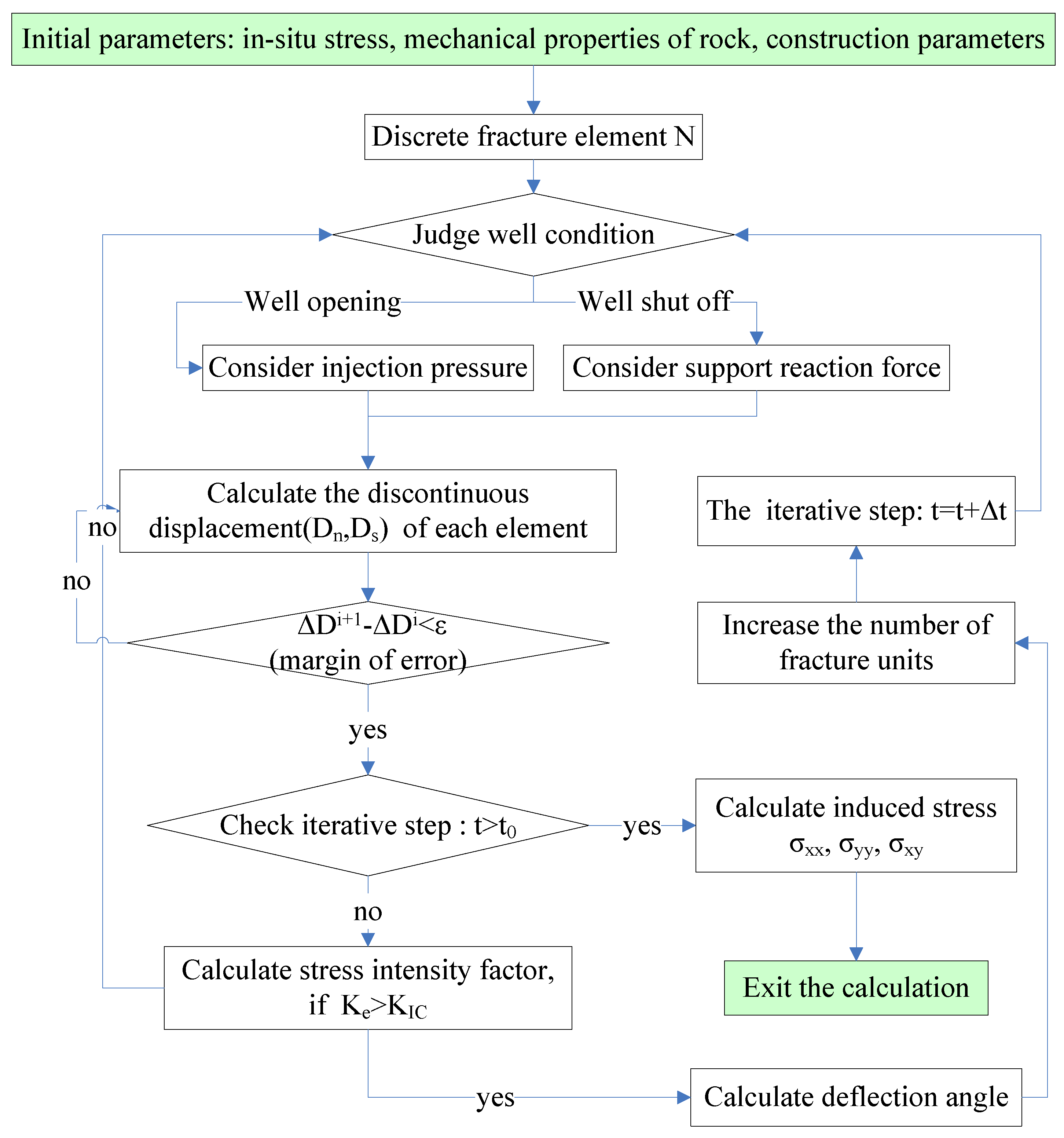
The stress intensity factor (SIF) is an important parameter to describe the field stress of the fracture tip, which is calculated by discontinuous displacement value on the fracture surface. The SIF in point a of the fracture tip can be shown [40]:
{ K I = 0.806 E π 4 ( 1 υ 2 ) 2 a D n K I I = 0.806 E π 4 ( 1 υ 2 ) 2 a D s
where K I and K I I is the stress intensity factor of different types of cracks, MPa∙m0.5; E is Young’s modulus, MPa; ν is Poisson’s ratio, and a is the half-length of crack, m.
At the same time, the maximum circumferential stress (MCS) criterion is introduced to judge the initiation and propagation direction of fracture [41]. The fracture deflection angle (θ0) can be obtained by solving the first-order partial derivative for the circumferential stress:
θ 0 = arcsin [ K I I ( K I + 3 K I 2 + 8 K I I 2 ) K I 2 + 9 K I I 2 ]
The mixed mode of the stress intensity factor is used to identify the initiation of HF and NFs:
K e = cos θ 0 2 [ K I cos 2 θ 2 3 2 K I I sin θ 0 ]
When K I C > K e , the fracture starts to propagate, where KIC is the fracture toughness, MPa∙m1/2.

2.5. Flowchart

The flow chart is shown in Figure 1. The solution procedure is as follows: ① Input initial parameters, such as maximum horizontal stress, minimum horizontal stress, Young’s modulus, Poisson’s ratio, fracture toughness, fracture number, fracture spacing, injection pressure, perforation depth, and perforating angle; ② Hydraulic fracture discretization and judge well condition; ③ Calculate the Dn and Ds of HF until the accuracy requirements are met by Equations (19)–(23) based on different well condition; ④ Check the iterative step, if the iterative step is greater than the preset value, calculate induced stress (Equation (5)) and exit the calculation, otherwise judge whether HF initiation occurs (Equation (26)); ⑤ If initiation occurs, calculate the deflection angle of the element (Equation (25)), increase fracture units and iterative step, and then go to step ②, else go to step ② directly.

2.6. Model Validation

Firstly, we verify the induced stress caused by fracture deformation. As the calculation model meets the plane strain condition [30], the analytical solution of the induced field stress around the fracture can be expressed as [42]:
{ σ x x = P f r a ( a 2 r 1 r 2 ) 3 2 sin θ sin [ 3 2 ( θ 1 + θ 2 ) ] P f [ r r 1 r 2 cos ( θ θ 1 + θ 2 2 ) 1 ] σ y y = P f r a ( a 2 r 1 r 2 ) 3 2 sin θ sin [ 3 2 ( θ 1 + θ 2 ) ] P f [ r r 1 r 2 cos ( θ θ 1 + θ 2 2 ) 1 ] σ x y = P f r a ( a 2 r 1 r 2 ) 3 2 sin θ cos [ 3 2 ( θ 1 + θ 2 ) ]
where Pf is the injection pressure, Pa; r, r1, r2 are respectively the distance between fracture and point Q, m; θ, θ1, θ2 are the angle between the x-axis and the line distance, °. The specific stress model is shown in Figure 2a:
Initial simulation parameters: injection pressure (Pf) is −3 MPa, the half-length of crack (a) is 1 m, the coordinates of point Q: x = 0.5 m, and y increases from 0 m to 10 m. Calculate the induced stress at point Q under a different vertical distance (coordinate y) from the fracture plane. The normal stress and shear stress obtained by simulation and calculation decrease with the increase of the distance from the fracture plane, and the numerical solution is basically consistent with the analytical solution. In Figure 2b, the solid line represents analytical results, and the dotted line represents the simulation results.
Secondly, we verify the stress intensity factor at the fracture tip. There is not only tensile failure, but also shear failure in the fracture, and the calculation model of the stress intensity factor at the fracture tip under the simple model is constructed (Figure 3). Assuming that there is a crack with a length of 2a in an infinitely uniform thin plate, the angle between fracture and the uniaxial tensile force P is θ. The calculation formula of the analytical solution of the stress intensity factor at the crack tip obtained by the Westergaard stress function method and the stress intensity factors of K I and K I I can be expressed as:
{ K I = P π a · sin 2 θ   K I I = P π a · sin θ · cos θ
In this paper, we calculated the stress intensity factors of K I and K I I at the tip of the fracture, where the analytical results about K I and K I I are respectively 1.3293 MPa∙m1/2 and 0.7765 MPa∙m1/2. In addition, at the same time, we provided the corresponding simulation results with different numbers of discrete elements. By comparing the simulation results with the analytical results, the relative error of our calculation model is obtained:
δ = (Kanal − Ksimu)/Kanal
where δ is the relative error, Kanal is analytical results, MPa∙m1/2, Ksimu is simulation results, MPa∙m1/2.
It can be seen from Table 1, as the number of discrete elements increases, the relative error decreases. The calculation accuracy can be guaranteed by increasing the number of discrete elements in numerical simulation. In the validation, a = 1 m, Pf = 1 MPa, θ = 60°.

3. Results and Discussion

The sequential fracturing model mentioned above is suitable for solving the mutual interference when the fractures are opened sequentially. In the following, we will talk about the fracture deformation and stress distribution in two kinds of sequential fracturing technology: one is about the staged fracturing technology in a single horizontal well, and the other is about sequential fracturing technology in a double horizontal well (zipper fracturing). The general range of values for parameters in numerical simulation can refer to our previous research [12]. The initial simulation parameters in this paper are as shown in Table 2.
In order to clearly display the propping effect of proppant on the fracture surface, we simulated the variation law of HF aperture during sequential fracturing of three HFs in a well, and revealed the responding mechanism of induced stress under proppant action. At the same time, we simulated the trajectory morphology under fracture interference during zipper fracturing. The specific physical model is as shown in Figure 4. Inject the fracturing liquid into HF 1 first, stop injection when HF 1 reaches the target length and then begin the fracturing construction on HF 2. Complete the fracturing of three HFs in this order.

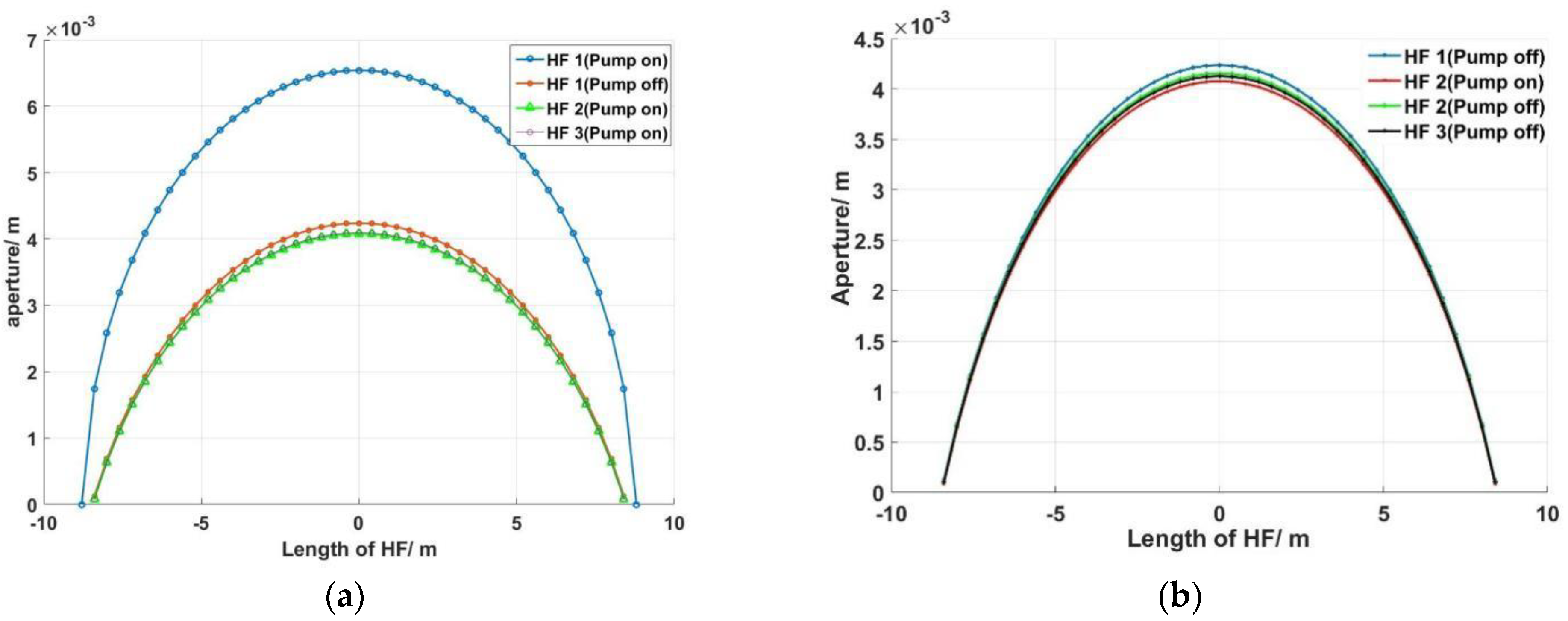
3.1. Deformation of Hydraulic Fracture and Induced Stress in a Single Well

The induced stress after hydraulic fracturing is mainly generated by the residual aperture of the fracture. Previous studies revealed that the induced compression stress around HF is always greater than anywhere else. Thus, in order to clearly reveal the interference mechanism from the previous hydraulic fracture completed by fracturing operation, we simulated the propagation of HF during staged fracturing first. Figure 5 shows the simulation results when hydraulic fracturing conduction is finished and three HFs reach equilibrium under in-situ stress.
From Figure 5, we can see that the deflection of hydraulic fractures in dynamic propagation may be affected by the HFs that have been fractured, and is away from the propped HF. Although the three fractures have the same injection pressure and are reached to balance under the same in-situ stress, induced stress produced by HF 1 is bigger than HF2, while HF 2 is bigger than HF 3. This is because, during the fracturing of HF 2 and 3, induced stress generated by propped fractures already exists, which leads to a gradual decrease in the maximum fracture aperture during subsequent hydraulic fracturing. The reduction of maximum HF aperture directly results in a reduction in proppant injection volume and residual aperture of HF.
In contrast, the fracturing HF may also affect the aperture of fractured HF. In order to quantitatively evaluate the aperture of HF 1 influenced by different fracturing stages, we conducted the following simulation, as shown in Figure 6.
Due to fracturing fluid filtration in HF, previously injected fracturing fluid cannot support HF to maintain initial maximum aperture. Comparing aperture of HF 1 under the situation of pump on and off of HF 1 in Figure 6a, we can see that, under the formation of compressive stress, the aperture of HF may have some retraction after hydraulic fracturing but will not be closed completely under proppant support. At the same time, if there is another HF that is under fracturing construction (HF 2 or 3), the induced stress generated by dynamic extension HF may compress HF 1 further (Figure 6a). However, from Figure 6b, we can see that, compared with HF 2 being pumped on, the aperture of HF 1 will have a weeny rebound after HF 2 is pumped off. The fracture residual width will decrease with an increasing number of stages, but the decrease is small and below 0.2 mm.

3.2. Sensitivity Analysis

We have analyzed the interaction mechanism of HFs in sequential fracturing above. However, the interaction degree is affected by many factors; therefore, a series of sensitivity analysis is carried out—the first is about the stiffness of proppant. We also quantitatively studied the residual aperture of HF under different stiffness of bracing member (Figure 7a). The induced stress caused by residual aperture of HF was shown in Figure 7b.
Simulation results showed that the support effect acting on the fracture surface is not linear. When the stiffness is less than 1 × 10¹⁰, the deformation of HF aperture is obvious. Conversely, when the stiffness is greater than 5 × 10¹⁰, the variation of residual HF aperture is not obvious. The greater the stiffness, the greater the influence of residual deformation on the in-situ stress after the fracture surface is closed.
In order to reveal the influence degree of this induced stress by residual aperture on subsequent HF deformation, based on the physical model as Figure 4a and Table 2, a numerical simulation study was carried out. Figure 8 is the simulation results about HF 2 with different stiffness and fracture spacing. To make the simulation results easy to compare, we did not display HF 1 temporarily.
From Figure 8a, we can see that the greater stiffness and the smaller fracturing spacing, the easier it is to cause subsequent fractures to be deflected. Bigger stiffness can keep larger residual aperture of HFs, and further produce bigger residual induced stress. This induced stress will deflect other fracture trajectories. However, the interference will decrease with the increase of fracture spacing (Figure 8b).

3.3. Deformation of HF and Distribution of Induced Stress under Zipper Fracturing

We have evaluated the influence of residual HF aperture in the above in staged fracturing when considering the reverse supporting force by proppant. Sequential fracturing not only exists in a single well, but also in multi-well fracturing. In this part, based on the sequential fracturing calculation model considering the supporting force of proppant in double wells, we simulated the propagation morphology of HF and characteristic of induced stress distribution in zipper fracturing. The physical model is as shown in Figure 4b, and the simulation results are shown in Figure 9. Well spacing is 70 m.
Simulation results in Figure 9 showed that, under the interference of adjacent fractures, hydraulic fractures tend to intersect among the two horizontal wells. In addition, at the same time, we should not ignore the existence of residual aperture of HF after fracturing. These residual apertures produced by proppant will exist for a long time and influence the propagation of subsequent HF. A series of sensitivity analyses were conducted to further investigate the influence mechanism of residual apertures on subsequent hydraulic fracture propagation.
From Figure 10, we can see that, with the decrease of well spacing and fracture spacing, HF 2 is more likely to deflect to HF 1. Setting a reasonable well spacing and fracturing spacing is beneficial for preventing the intersection of HF in adjacent wells. Compared to fracture spacing, the deflection of HF 2 is influenced by well spacing.

4. Conclusions

In this paper, a hydraulic fracture propagation model was established, which considered the influence of residual fracture aperture on subsequent hydraulic fracture propagation. The interaction of hydraulic fractures during sequential fracturing is studied by a series of numerical simulations:
(1)
As large quantities of proppant are injected into hydraulic fracture during hydraulic fracturing, fractures will not completely close after the fracturing operation is completed. This residual aperture caused by proppant may produce induced stress and change the distribution of in-situ stress. Induced stress by residual aperture gradually decreases with the increase of vertical distance from the fracture plane and the decrease of residual aperture of fracture.
(2)
The residual aperture will also influence the propagation and maximum aperture of subsequent fracture. When the fracture spacing in sequence fracturing is closer, the residual aperture will inhibit the opening degree of the subsequent fracture, which in turn affects the injection volume of the proppant. During sequence fracturing, fractures tend to exclusion and turn away in staged fracturing, on the contrary, which tends to approach and intersect in zipper fracturing.
(3)
Subsequent fracturing in turn compresses the previously cracked fracture, resulting in a further reduction in residual aperture, and after the fracture construction is completed, the previously pressurized fracture aperture is rebound. As the number of hydraulic fracture increases, the residual aperture of the previously pressed fracture gradually decreases. However, the fluctuation of fracture aperture mentioned above is small and less than 0.2 mm.
(4)
Sensitivity analysis shows that, in staged fracturing, the smaller the fracturing spacing, the more likely subsequent fractures are to be deflected, while in zipper fracturing, the effect of fracture spacing is not obvious. Well spacing can obviously influence the deflection of subsequent fracture in zipper fracture. With the increase of stiffness, the residual aperture of the hydraulic fracture increases, and the subsequent fractures are more likely to be deflected.
There are still some shortcomings in this paper. For example, the proppant stiffness is still fixed, which cannot reflect the nonlinear propping effect of proppant on fracture surfaces. At the same time, the fracturing fluid filtration process in the fracture is not considered. In the future, we will focus on optimizing these deficiencies and coupling them with existing models.

Author Contributions

Conceptualization, P.Z.; Data curation, P.Z.; Formal analysis, P.Z.; Funding acquisition, D.Z.; Investigation, T.G. and E.L.; Methodology, M.Z.; Software, P.Z.; Validation, D.Z.; Writing—original draft, P.Z.; Writing—review and editing, P.Z. All authors have read and agreed to the published version of the manuscript.

Funding

This work was supported by the National Natural Science Foundation of China (51934005, 51874242).

Informed Consent Statement

Not applicable.

Data Availability Statement

The data presented in this study are available on request from the corresponding author.

Conflicts of Interest

The authors declare no conflict of interest.

References

  1. British Patroleum. Statistical Review of World Energy; BP: London, UK, 2021. [Google Scholar]
  2. Khormali, A.; Petrakov, D.G.; Lamidi, A.-L.B. Prevention of Calcium Carbonate Precipitation during Water Injection into High-Pressure High-Temperature Wells. In Proceedings of the SPE European Formation Damage Conference and Exhibition, Budapest, Hugary, 3–5 June 2015. [Google Scholar]
  3. Khormali, A.; Bahlakeh, G.; Struchkov, I.; Kazemzadeh, Y. Increasing inhibition performance of simultaneous precipitation of calcium and strontium sulfate scales using a new inhibitor—Laboratory and field application. J. Pet. Sci. Eng. 2021, 202, 108589. [Google Scholar] [CrossRef]
  4. Khormali, A.; Sharifov, A.R.; Torba, D.I. Experimental and modeling analysis of asphaltene precipitation in the near wellbore region of oil wells. Pet. Sci. Technol. 2018, 36, 1030–1036. [Google Scholar] [CrossRef]
  5. Wang, Y.; Ju, Y.; Zhang, H.; Gong, S.; Song, J.; Li, Y.; Chen, J. Adaptive Finite Element-Discrete Element Analysis for the Stress Shadow Effects and Fracture Interaction Behaviours in Three-Dimensional Multistage Hydrofracturing Considering Varying Perforation Cluster Spaces and Fracturing Scenarios of Horizontal Wells. Rock Mech. Rock Eng. 2021, 54, 1815–1839. [Google Scholar] [CrossRef]
  6. Zhou, D.; Zheng, P.; Yang, J.; Li, M.; Xia, Y.; Cai, W.; Ma, X.; Liu, S. Optimizing the construction parameters of modified zipper fracs in multiple horizontal wells. J. Nat. Gas Sci. Eng. 2019, 71, 102966. [Google Scholar] [CrossRef]
  7. Yang, Z.Z.; He, R.; Li, X.; Li, Z.; Liu, Z.; Lu, Y. Application of Multi-Vertical Well Synchronous Hydraulic Fracturing Technology for Deep Coalbed Methane (DCBM) Production. Chem. Technol. Fuels Oils 2019, 55, 299–309. [Google Scholar] [CrossRef]
  8. Li, J.X.; Dong, S.; Hua, W.; Yang, Y.; Li, X. Numerical Simulation on Deflecting Hydraulic Fracture with Refracturing Using Extended Finite Element Method. Energies 2019, 12, 2044. [Google Scholar] [CrossRef] [Green Version]
  9. Guo, T.; Zhang, Y.; Zhang, W.; Niu, B.; He, J.; Chen, M.; Yu, Y.; Xiao, B.; Xu, R. Numerical simulation of geothermal energy productivity considering the evolution of permeability in various fractures. Appl. Therm. Eng. 2022, 201, 117756. [Google Scholar] [CrossRef]
  10. Zhu, H.; Tang, X.; Song, Y.; Li, K.; Xiao, J.; Dusseault, M.B.; McLennan, J.D. An Infill Well Fracturing Model and Its Microseismic Events Barrier Effect: A Case in Fuling Shale Gas Reservoir. SPE J. 2021, 26, 113–134. [Google Scholar] [CrossRef]
  11. Ren, X.; Zhou, L.; Zhou, J.; Lu, Z.; Su, X. Numerical analysis of heat extraction efficiency in a multilateral-well enhanced geothermal system considering hydraulic fracture propagation and configuration. Geothermics 2020, 87, 101834. [Google Scholar] [CrossRef]
  12. Zheng, H.; Pu, C.; Xu, E.; Sun, C. Numerical investigation on the effect of well interference on hydraulic fracture propagation in shale formation. Eng. Fract. Mech. 2020, 228, 106932. [Google Scholar] [CrossRef]
  13. Guo, T.; Wang, X.; Li, Z.; Gong, F.; Lin, Q.; Qu, Z.; Lv, W.; Tian, Q.; Xie, Z. Numerical simulation study on fracture propagation of zipper and synchronous fracturing in hydrogen energy development. Int. J. Hydrog. Energy 2019, 44, 5270–5285. [Google Scholar] [CrossRef]
  14. Zheng, P.; Zhou, D. Study on fracture propagation and interaction mechanism during hydraulic fracturing. IOP Conf. Ser. Earth Environ. Sci. 2021, 621, 012134. [Google Scholar] [CrossRef]
  15. Zheng, P.; Xia, Y.; Yao, T.; Jiang, X.; Xiao, P.; He, Z.; Zhou, D. Formation mechanisms of hydraulic fracture network based on fracture interaction. Energy 2022, 243, 1–16. [Google Scholar] [CrossRef]
  16. Zhang, Z.; Zhang, S.; Zou, Y.; Ma, X.; Li, N.; Liu, L. Experimental investigation into simultaneous and sequential propagation of multiple closely spaced fractures in a horizontal well. J. Pet. Sci. Eng. 2021, 202, 108531. [Google Scholar] [CrossRef]
  17. Ju, Y.; Li, Y.; Wang, Y.; Yang, Y. Stress shadow effects and microseismic events during hydrofracturing of multiple vertical wells in tight reservoirs: A three-dimensional numerical model. J. Nat. Gas Sci. Eng. 2020, 84, 103684. [Google Scholar] [CrossRef]
  18. Sobhaniaragh, B.; Trevelyan, J.; Mansur, W.J.; Peters, F.C. Numerical simulation of MZF design with non-planar hydraulic fracturing from multi-lateral horizontal wells. J. Nat. Gas Sci. Eng. 2017, 46, 93–107. [Google Scholar] [CrossRef] [Green Version]
  19. Sukumar, S.; Weijermars, R.; Alves, I.; Noynaert, S. Analysis of Pressure Communication between the Austin Chalk and Eagle Ford Reservoirs during a Zipper Fracturing Operation. Energies 2019, 12, 1469. [Google Scholar] [CrossRef] [Green Version]
  20. Li, S.; Zhang, D. A Fully Coupled Model for Hydraulic-Fracture Growth During Multiwell-Fracturing Treatments: Enhancing Fracture Complexity. In Proceedings of the SPE Reservoir Simulation Conference, Montgomery, TX, USA, 20–22 February 2017. [Google Scholar]
  21. Kumar, D.; Ghassemi, G. A three-dimensional analysis of simultaneous and sequential fracturing of horizontal wells. J. Pet. Sci. Eng. 2016, 146, 1006–1025. [Google Scholar] [CrossRef]
  22. Kumar, D.; Ghassemi, A. Three-Dimensional Poroelastic Modeling of Multiple Hydraulic Fracture Propagation from Horizontal Wells. Int. J. Rock Mech. Min. Sci. 2018, 105, 192–209. [Google Scholar] [CrossRef]
  23. Chen, X.; Li, Y.; Zhao, J.; Xu, W.; Fu, D. Numerical investigation for simultaneous growth of hydraulic fractures in multiple horizontal wells. J. Nat. Gas Sci. Eng. 2018, 51, 44–52. [Google Scholar] [CrossRef]
  24. Wang, Z.; Yang, L.; Gao, R.; Xu, G.; Liu, X.; Mo, S.; Fan, M.; Wang, X. Numerical Analysis of Zipper Fracturing Using a Non-Planar 3D Fracture Model. Front. Earth Sci. 2022, 10, 808183. [Google Scholar] [CrossRef]
  25. Xu, W.; Zhao, J.; Rahman, S.S.; Li, Y.; Yuan, Y. A Comprehensive Model of a Hydraulic Fracture Interacting with a Natural Fracture: Analytical and Numerical Solution. Rock Mech. Rock Eng. 2018, 52, 1095–1113. [Google Scholar] [CrossRef]
  26. Li, K.; Huang, L.-h.; Huang, X.-c. Propagation simulation and dilatancy analysis of rock joint using displacement discontinuity method. J. Cent. South Univ. 2014, 21, 1184–1189. [Google Scholar] [CrossRef]
  27. Cheng, W.; Jiang, G.; Jin, Y. Numerical simulation of fracture path and nonlinear closure for simultaneous and sequential fracturing in a horizontal well. Comput. Geotech. 2017, 88, 242–255. [Google Scholar] [CrossRef]
  28. Atkinson, B.K. Fracture Mechanics of Rock; Academic Press: London, UK, 1987. [Google Scholar]
  29. Geertsma, J.; De Klerk, F. A rapid method of predicting width and extent of hydraulically induced fractures. J. Pet. Technol. 1969, 21, 1571–1581. [Google Scholar] [CrossRef]
  30. Kim, J.-H.; Paulino, G.-H. On Fracture Criteria for Mixed-Mode Crack Propagation in Functionally Graded Materials. Mech. Adv. Mater. Struct. 2007, 14, 227–244. [Google Scholar] [CrossRef]
  31. Cheng, W.; Jin, Y.; Chen, M. Reactivation mechanism of natural fractures by hydraulic fracturing in naturally fractured shale reservoirs. J. Nat. Gas Sci. Eng. 2015, 23 Pt P3, 431–439. [Google Scholar] [CrossRef]
  32. Crouch, S.L. Solution of plane elasticity problems by the displacement discontinuity method. I. Infinite body solution. Int. J. Numer. Methods Eng. 1976, 10, 301–343. [Google Scholar] [CrossRef]
  33. Crouch, S.L.; Starfield, A.M. Boundary Element Methods in Solid Mechanics; Goerge Allen and Unwin: London, UK, 1983. [Google Scholar]
  34. Chen, X.; Zhao, J.; Li, Y.; Yan, W.; Zhang, X. Numerical Simulation of Simultaneous Hydraulic Fracture Growth Within a Rock Layer: Implications for Stimulation of Low-Permeability Reservoirs. J. Geophys. Res. Solid Earth 2019, 124, 13227–13249. [Google Scholar] [CrossRef]
  35. Le Calvez, J.H.; Craven, M.E.; Klem, R.C.; Baihly, J.D.; Bennett, L.A.; Brook, K. Real-time microseismic monitoring of hydraulic fracture treatment: A tool to improve completion and reservoir management. In Proceedings of the SPE Hydraulic Fracturing Technology Conference (Society of Petroleum Engineers), College Station, TX, USA, 29–31 January 2007. [Google Scholar]
  36. Cheng, W.; Gao, H.; Jin, Y.; Chen, M.; Jiang, G. A study to assess the stress interaction of propped hydraulic fracture on the geometry of sequential fractures in a horizontal well. J. Nat. Gas Sci. Eng. 2017, 37, 69–84. [Google Scholar] [CrossRef]
  37. Goodman, R.E.; Taylor, R.L.; Brekke, T.L. A Model for the Mechanics of Jointed Rock. J. Soil Mech. Found. Div. 1968, 94, 637–659. [Google Scholar] [CrossRef]
  38. Zhou, J.; Zhang, L.; Qi, S.; Yang, D. Empirical ratio of dynamic to static stiffness for propped artificial fractures under variable normal stress. Eng. Geol. 2020, 273, 105683. [Google Scholar] [CrossRef]
  39. Indraratna, B.; Oliveira, D.A.F.; Brown, E.T. A shear-displacement criterion for soil-infilled rock discontinuities. Géotechnique 2010, 60, 623–633. [Google Scholar] [CrossRef]
  40. Olson, J.E. Fracture aperture, length and pattern geometry development under biaxial loading: A numerical study with applications to natural, cross-jointed systems. Geol. Soc. Lond. Spec. Publ. 2007, 289, 123–142. [Google Scholar] [CrossRef]
  41. Erdogan, F.; Sih, G.C. On The Crack Extension in Plates Under Plane Loading and Transverse Shear. J. Basic Eng. 1963, 85, 519–525. [Google Scholar] [CrossRef]
  42. Sneddon, I.N.; Elliott, H.A. The opening of a Griffith crack under internal pressure. Q. Appl. Math. 1946, 4, 262–267. [Google Scholar] [CrossRef] [Green Version]
Figure 1. Computer program flow chart.
Processes 10 00937 g001
Figure 2. Validation of simulation model. (a) mechanical model; (b) comparison of simulation results; “*” represents the numerical solution, solid lines represent analytical solutions.
Processes 10 00937 g002
Figure 3. The mechanical model. Where: θ is the angle between fracture and the uniaxial tensile force P.
Processes 10 00937 g003
Figure 4. Physical model of sequential fracturing (a) in a single horizontal well; (b) in a double horizontal well, where: d1 represents the perforating depth and d2 represents the fracturing spacing in a well, and d3 represents well spacing. Ph and PH represent the minimum and maximum horizontal principal stress sequentially. Hydraulic fracture number represents the fracturing sequence.
Processes 10 00937 g004
Figure 5. Numerical simulation results of fracture morphology and induced stress of (a) σxx produced by residual aperture after completion of fracturing stage 1; (b) σxx produced by residual aperture after completion of fracturing stage 2; (c) σxx produced by residual aperture after completion of fracturing stage 3; (d) σxy produced by residual aperture after completion of fracturing stage 1.
Processes 10 00937 g005
Figure 6. Aperture of hydraulic fracture 1. (a) in different fracturing stages; (b) in different shut off stages of the well.
Processes 10 00937 g006
Figure 7. (a) Aperture of HF 1 with different stiffness; (b) induced stress near the fracture surface.
Processes 10 00937 g007
Figure 8. Deformation results about HF 2. (a) with different stiffness at constant fracture spacing; (b) with different fracture spacing at constant stiffness.
Processes 10 00937 g008
Figure 9. Numerical simulation results of fracture morphology and induced stress of (a) σxx produced by residual aperture after completion of fracturing; (b) σxy produced by residual aperture.
Processes 10 00937 g009
Figure 10. Simulation results of (a) the deflection of HF 2 with different well spacing; (b) the deflection of HF 2 with different fracture spacing. Where: the solid line on Well 2 represents HF 2 at different fracture spacing. The colors of HF 1 and HF 2 are corresponding at different spacing.
Processes 10 00937 g010
Table 1. Relative errors of I-type and II-type stress intensity factors at the crack tip.
Element Number K I / ( M P a · m 1 / 2 ) (Analytical Results, 1.3293) K I I / ( M P a · m 1 / 2 ) (Analytical Results, 0.7765)
The Relative Error S i m u l a t i o n   R e s u l t s The Relative Error S i m u l a t i o n   R e s u l t s
r5.0%1.26226.1%0.7288
42.1%1.30163.2%0.7515
61.1%1.31512.1%0.7593
100.2%1.32611.4%0.7657
Table 2. Initial simulation parameters.
Young’s modulus (MPa)19,830Minimum horizontal stress (MPa)−20
Poisson’s ratio0.261Fracture toughness (MPa·m1/2)2.5
Maximum horizontal stress (MPa)−24Injection pressure (MPa)−20
Injection angle (°)90Fracturing cluster number3
Fracture spacing(m)40Perforating depth (m)1
Publisher’s Note: MDPI stays neutral with regard to jurisdictional claims in published maps and institutional affiliations.

