Article

Targeting on Different Characteristic Continuous Variables in Process Transition for Ethylene Column with Wide-Range Feed Fluctuation

Department of Automation, China University of Petroleum, Beijing 102249, China
*
Author to whom correspondence should be addressed.
Processes 2022, 10(4), 796; https://doi.org/10.3390/pr10040796
Submission received: 26 February 2022 / Revised: 15 April 2022 / Accepted: 15 April 2022 / Published: 18 April 2022
(This article belongs to the Topic Bioreactors: Control, Optimization and Applications)

Abstract

:
For the study of the transition strategies of continuous chemical processes, both continuity and dynamic characteristics in the physical sense are critical. The continuous transition strategy has a higher information density and can describe the real situation as closely as possible. In addition, the accuracy of the dynamic characteristics is necessary because the process transition is the study of the dynamic system processes. However, existing transition strategies have certain shortcomings. Dynamic optimization can obtain transition strategies with different characteristics but no physical meaning and a frequency domain-based analytical approach can acquire a continuous transition strategy with physical meaning, but its dynamic characteristics are the same. Therefore, by integrating the advantages of the existing strategies, a new transition strategy has been presented, which possesses different dynamic characteristics and continuity synchronous with physical significance. When process transition occurs, the proposed strategy results in less fluctuation and can quickly reach and maintain a steady state. Furthermore, the strategy is also suitable for the rapid application of different transition processes in the same plant. The performance of the transition strategies is evaluated through research on a continuous feed ethylene column.

1. Introduction

The complicated process industry occupies an essential position in the industrial system and national economy [1]. In recent years, the shortage of resources and the intensification of market competition have urged process industries to meet higher demands for product quality, security, cost, and efficiency [2,3,4,5].
As a crucial part of the process industry, chemical processes are often accompanied by the problems of variable production conditions [6], complexity mechanisms [7,8], and huge consumption of raw materials and energy [9]. When production demands change, the operating conditions change accordingly [10,11], and large-scale operating changes are called process transition. In the process transition of the chemical industry, the conventional process control strategies, such as PID control, find it difficult to make smooth working condition transitions, owing to the complicated process mechanisms. The existence of a large number of non-stationary changes may cause the production indicators to be far from the target, thereby affecting the final product quality and production costs [12,13]. Therefore, it is necessary to explore effective process transition strategies to achieve a smooth transition of working conditions and avoid wasting materials and energy.
At present, the solution paradigms for process transition strategies are largely concentrated on the optimization-based and analysis-based methods. The optimization approach transforms transition problems into a general dynamic optimization issue, and then receives the manipulated variable transition trajectory by solving the specific objective function. For example, Aydin et al. [14] proposed the combination of an indirect solution scheme together with a parsimonious input parametrization to address the dynamic optimization of batch and semi-batch chemical processes. Huang et al. [15] developed a method based on control vector parameterization (CVP) to obtain the transition trajectory during the transition process of working conditions in ethylene columns.
The analytical method obtains the corresponding relationship between the manipulated variable and system model by analyzing the essence of the transition problem, and then directly deduces the manipulated variable transition trajectory through the system model, such as Cao et al. [16] presented in a frequency domain-based analytical approach. It acquires the continuous transition strategy with physical significance through the transfer function model, which is unable to be addressed in the time domain. Although the continuous transition strategy can achieve some improvements in transition performance, it has two shortcomings: (1) as a nonlinear system, the majority of practical processes need to obtain the transfer function through linearization; (2) the calculation in the frequency domain ignores the dynamic differences between the manipulated variables. These operations simplify the solution process of the transition problem and provide a feasible solution for studying the continuous process transition strategy of complex systems. Nonetheless, excessive simplification results in the lack of some dynamic characteristics of manipulated variables, which will have some negative impact on the transition process.
To sum up, this paper has some innovations as follows: a new process transition strategy has been developed by integrating the advantages of the existing process transition strategy. When process transition occurs, it has less fluctuation than conventional approaches and can quickly reach and maintain a steady state. Furthermore, for different transition processes of the same process plant, it can be quickly applied to other transition processes through parameter optimization. A common ethylene distillation column as a benchmark case is used to evaluate the performance of the transition strategies.
The organization of the paper is as follows: the deficiencies of the existing transition strategy are introduced in Section 2; in Section 3, the proposed transition strategy is described in detail and applied to the transition problem of ethylene columns; the rapid application of the method in different transition processes is explored in Section 4; finally, the conclusion is drawn in Section 5.

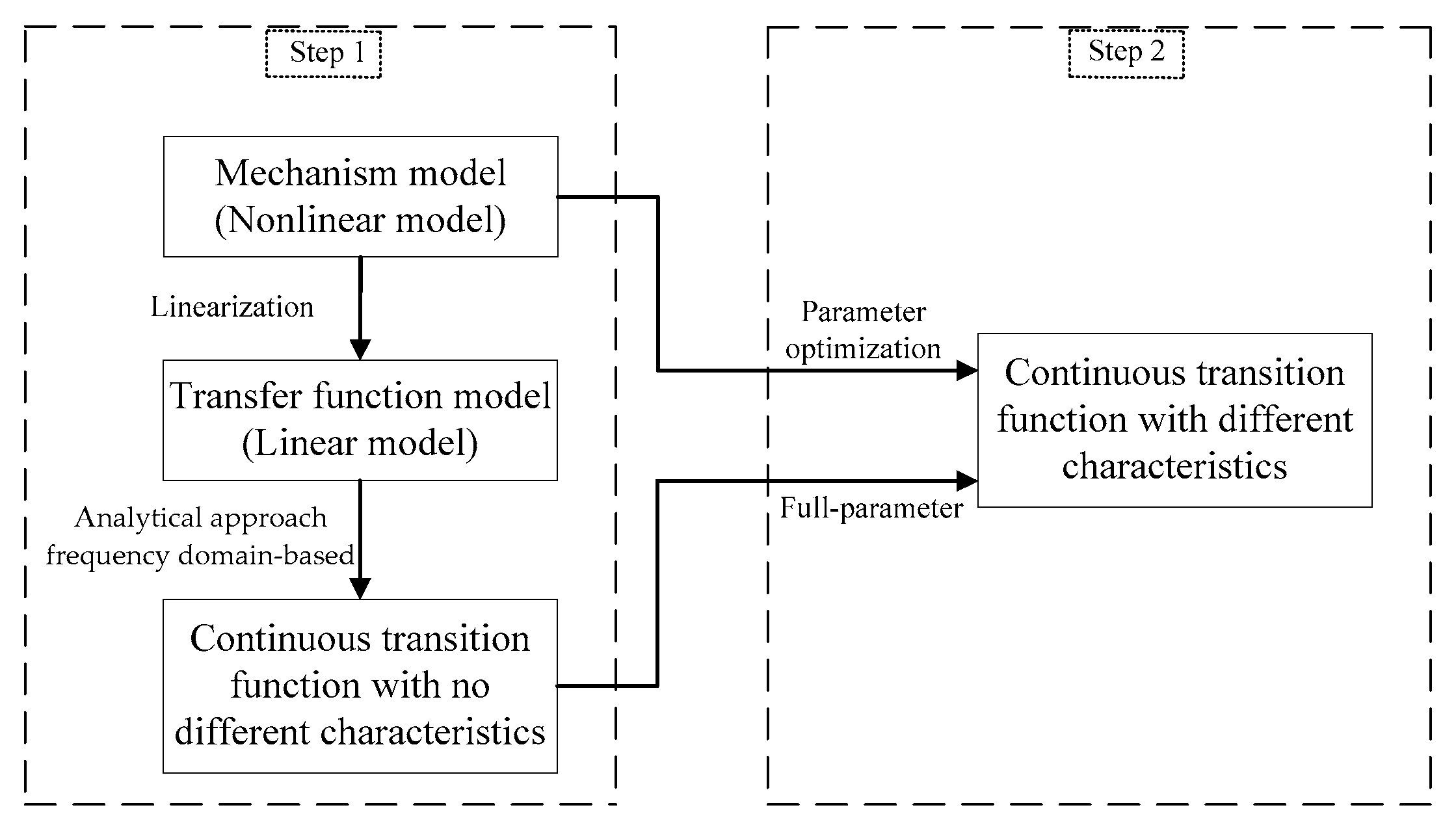
2. Problem Presentation

Against the background of the variable production conditions in chemical processes, wide-range process transitions occur from time to time due to the change of work demands [17] and the process transition strategy is the transition method aimed at this process.

2.1. Process Transition Strategy with Different Characteristics

Process transition cannot happen without changing the driving variables. A driving variable refers to the variable that can cause the process transition of a system. All variables will remain constant when the system is running at steady state. Therefore, there must be a kind of variable in the system that can vary initiatively, that is, driving variables, so that the current steady state can be broken. The system enters the transition state after the driving variable starts to change, and the production indicator deviates from the expectation. The corresponding manipulated variable should also start to vary immediately to compensate for the deviation of the production indicator caused by the variation of the driving variable. The transition strategy is mainly to find the appropriate transition trajectories of the manipulated variables to make the process plant meet the requirement of the production indicators.
Process transition is the study of a system’s dynamic processes, so the transition issue can be regarded as a dynamic optimization issue. The dynamic process is generally described by differential and algebraic equations (DAE), and dynamic optimization is a common way to address the dynamic programming problem with DAE constraints. Subsequently, under the constraints of the physical model of the plant, the transition trajectory of the manipulated variable is computed by minimizing the given objective function. For this, the general paradigm of the optimization problem (defined Model 1) is given and the description of each variable is shown in Table 1.
m i n u t                     J = Φ x t , u t , d t , t f s . t .           x ˙ t = f x x t , u t , d t d t = d * t x t 0 = x t 0 ,           x t f = x t f u t 0 = u t 0 ,           u t f = u t f
The advantages and disadvantages of the dynamic optimization method are obvious. The advantage lies in the ability to solve an optimal transition trajectory of the manipulated variable for a specific transition process. For continuous processes, as long as the target operating point exists, a transition trajectory that fits the demand can generally be obtained through dynamic optimization. That is to say, the dynamic optimization has a wider application range [18,19].
However, the disadvantage of dynamic optimization is that it is almost impossible for complex systems to obtain an analytical solution through the indirect method [20,21]. Therefore, the direct method is generally adopted to transform the original optimization problems to the nonlinear programming problems by discretization [22,23]. The common methods are those such as control vector parameterization and orthogonal collocation. Although the direct method can address the complicated problem, it is obvious that the obtained input variables, that is, the manipulated variables, are piecewise functions [24]. The essence of the direct method is to acquire the optimal input through piecewise approximation. Piecewise functions are generally discontinuous, but some input parameterization methods can be used to ensure the smoothness of the solution, and then a continuous input function can be acquired. However, we do not know what the optimal solution looks like before the calculation, so the approximation function is generally selected based on experience. It means that dynamic optimization is to numerically approach the optimal solution piecewise. Even if a continuous input function can be obtained, it has no physical meaning. For piecewise functions through numerical approximation, some partial details may be ignored due to the influence of discrete precision, which may have some negative effects on control performance for continuous industrial processes. While the problem can be addressed by raising the discrete accuracy, the increase in discrete accuracy leads to an increase in calculation cost. The excessive computational costs bring great challenges to practical applications [25]. For some partial variations with a short duration, the raise in discrete accuracy indefinitely is unrealistic.

2.2. Continuous Process Transition Strategy with No Different Characteristics

It can be seen from the above analysis that there are two defects in dynamic optimization in the research of the transition strategy of complex systems: it is difficult to solve by the indirect method and a continuous solution with physical significance cannot be obtained by the direct method. Cao et al. [16] presented the frequency domain-based analytical approach (A-FD) to overcome the shortcomings of the dynamic optimization method, which is shown in Figure 1.
Different from the optimization idea, the A-FD maps the transition problem from the time domain to the frequency domain space, and then directly solves the continuous transition trajectory of the manipulated variables according to the transfer function model of the plant in the frequency domain space. A transfer function model consisting of algebraic equations is used to describe the plant in place of differential algebraic equations. The computational difficulty of transition problems is reduced, making it possible to find continuous analytical solutions to complex problems. The advantage of the A-FD is that for complicated systems, continuous transition trajectories can still be obtained without numerical approximation by basic functions. The acquired manipulated variable therefore has actual physical significance.
Nevertheless, the A-FD also has two shortcomings. Firstly, actual industrial processes are generally nonlinear. The A-FD needs to transform the nonlinear physical model of the plant into the linear transfer function model by linearization. The linearization of the nonlinear model is carried out at a certain working point, and the obtained transfer function is essentially the model at this working point rather than that of the entire transition process [26]. Using the transfer function model at a certain working point to replace that of the entire transition process for calculation will bring certain errors to the transition strategy. Secondly, the computation in the frequency domain is based on an assumption that the dynamic characteristics of each manipulated variable are identical during the transition process, which ignores the dynamic differences between manipulated variables. In the actual process, because the system responds differently to different manipulated variables, the dynamic characteristics of each manipulated variable cannot be exactly the same in the dynamic process. Since process transition is the study of dynamic system processes, the dynamic characteristics of the transition strategy are crucial. It is necessary to be employed on the basis of the characteristics of the manipulated variable itself to acquire a better adjustment effect in line with reality. The transition strategy acquired under the condition of ignoring the difference in dynamic characteristics is obviously not optimal.
In contrast to dynamic optimization, the A-FD can obtain the continuous transition trajectory of manipulated variables with physical meaning, which has an important practical value for the transition strategy. Nevertheless, the continuous transition strategy with no different characteristics can be achieved due to the limitations of the solution method, which does not conform to the dynamic characteristics of the actual process. In other words, the A-FD is not the optimal solution for the process transition strategy. Therefore, studying new methods to obtain the optimal transition strategy is necessary, that is, a continuous transition strategy with different characteristics. For the convenience of explanation, the continuity in the following refers to the continuity with physical meaning.

3. Continuous Process Transition Strategy with Different Characteristics

In this section, for the research on the transition strategy of complex systems, the accuracy of the transition strategy will be improved by improving the solution method, while considering the challenge brought by the computational cost.

3.1. Solution Method of Continuous Process Transition Strategy with Different Characteristics

Since dynamic optimization cannot obtain physically meaningful transition strategies, improvement on the basis of the A-FD was considered, in order to obtain the continuous transition strategy with different characteristics. For the continuous transition strategy acquired through the previous A-FD, the transition functions of manipulated variables are generally signified as
u ( t ) = f u k , T , k 0 = u 1 t u 2 t u l t u M t T k = k 1 , 1 k 1 , 2 k 1 , r k 1 , N k 2 , 1 k 2 , 2 k 2 , r k 2 , N k l , 1 k l , 2 k l , r k l , N k M , 1 k M , 2 k M , r k M , N T = T 1 , 1 T 1 , 2 T 1 , r T 1 , N T 2 , 1 T 2 , 2 T 2 , r T 2 , N T l , 1 T l , 2 T l , r T l , N T M , 1 T M , 2 T M , r T M , N k 0 = k 1 , 0 k 2 , 0 k l , 0 k M , 0 T = u t 0 k = k 1 ; k 2 ; k l ; k M M × N , T = T 1 ; T 2 ; T l ; T M M × N
where f u represents the equation of manipulated variables. k 0 signifies the initial steady-state value of manipulated variables, that is, u t 0 . k and T express the steady and dynamic parameter matrices in the transition function of the manipulated variables, respectively. u l t signifies the lth manipulated variable of u t , k l and T l represent the parameters of u l t . k l , r and T l , r express the rth steady and dynamic parameters of u l t , respectively. k l , 0 represents the initial steady-state value of u l t .
The A-FD assumes the same dynamic characteristics for each manipulated variable. In brief, no matter how many manipulated variables there are, only one set of steady and one set of dynamic parameters is calculated. There is no difference between manipulated variables, which can be signified as
k 1 = k 2 = = k l = = k M T 1 = T 2 = = T l = = T M
However, there are certain differences between the optimal transition trajectories in practical problems because the plant response to diverse manipulated variables is different. The transition function of each manipulated variable should have a unique set of parameters. Solving the continuous transition strategy with different characteristics is transformed into solving the manipulated variable transition function with different parameters.
In fact, the A-FD acquires the continuous transition strategy with no different characteristics, while dynamic optimization obtains the transition strategy with different characteristics. In other words, the superiorities of the two methods are obvious and complementary. Thereby, for the continuous transition functions with the same parameters which are obtained from the A-FD, the optimal transition trajectory of each manipulated variable can be acquired by optimizing all parameters of continuous functions. The optimized transition functions have different parameters, resulting in a continuous transition strategy with different characteristics. The optimization problem can be expressed as Model 2:
m i n k , T J = Φ x t , u t , d t , t f s . t . x ˙ t = f x x t , u t , d t u t = f u k , T , k 0 d t = d * t k 0 = u t 0 x t 0 = x t 0 , x t f = x t f u t 0 = u t 0 , u t f = u t f
Compared with optimization Model 1, the optimization variables in Model 2 only involve the parameters of continuous function, thus there is no need for handling with discretization. In addition, the optimization in the time domain is to directly calculate the mechanism model of the process plant, while avoiding the error attributed to the linearization of a nonlinear model. The new approach for the process transition strategy, which combines the optimization method and analytical method, can be called the two-step optimization frequency domain-based approach (TSO-FD). The schematic diagram of the proposed method is shown in Figure 2.
The TSO-FD will be implemented in two steps. In the first step, the nonlinear mechanism model is transformed into the linear transfer function model by linearization, meanwhile the transition problem in the time domain is transformed into that in the frequency domain. Then, the transition problem in the frequency domain is solved by analytical method to achieve the continuous transition trajectories of the manipulated variables with physical meaning. The second step is to adjust all parameters of continuous function through parameter optimization based on the original nonlinear mechanism model to acquire the continuous transition trajectories with different characteristics.
The TSO-FD integrates the virtues of the A-FD and dynamic optimization. That is, the continuous transition strategy with physical significance is acquired through the idea of the analytical method, and the transition strategy with different characteristics is obtained through the idea of the optimization method, so that the continuous transition strategy with different characteristics is finally received. Both continuity and dynamic characteristics in the physical sense are critical for transition strategy. It is foreseeable that compared with the existing transition strategies, the performance will be better for the transition strategy that simultaneously has continuity with physical meaning and different characteristics. It has important guiding significance for the chemical process transition with high production indicator requirements.
It is important to notice that as the foundation of the study, the transfer function is the common mathematical model to describe linear processes. However, the majority of practical processes are inherently nonlinear. For weakly nonlinear processes, adequate analytical accuracy can be acquired by describing approximately the nonlinear behavior through linearization approaches. However, the linearization of strongly nonlinear processes may bring great errors, resulting in the inability to accurately analyze the dynamic characteristics of the processes. That is, the presented approach applies to process transitions of weakly nonlinear processes, but not strongly nonlinear processes.

3.2. Transition Strategy for Ethylene Column

Distillation is a common separation technology in chemical industry production and is applied in approximately 95% of fluid separation manipulations [27,28]. For ethylene production systems, the distillation column is essential equipment, used to refine the ethylene product by the mass exchange and heat exchange processes of the gas and liquid phase. This distillation process only involves physical changes, and the nonlinearity level is not high, so it can be considered as a weakly nonlinear process. The ethylene column has the feature of high product quality demands, complicated dynamic characteristics, and more interference factors. There is a need for precise operation and regulation of ethylene columns [29,30,31]. Thus, the research in transition strategy by taking the ethylene column for a case is appropriate and representative.
An in-service ethylene column was selected as a benchmark case, as exhibited in Figure 3. The upstream cracking furnace group produces overheated cracking gas as feed to the ethylene column, and the feed contains four components, ethane, ethylene, and a little hydrogen and methane. The ethylene product is drawn from the side at the top, and the ethane product is drawn from the bottom. The cracking furnaces will be coking after running for a while. Each cracking furnace in the group should be down regularly for cleaning in sequence and then put into operation again. It means that the feed of the ethylene column will fluctuate on a large scale periodically, and consequently cause variations in operating conditions, that is, process transition. The ethylene column dynamic model has been established by our research group. The model takes into account not only the dynamic process of the gas and liquid phase on the tray but also the dynamic characteristics of the gas holdup in the vapor space and the liquid holdup in the downcomer [32]. Considering the high efficiency of the process simulation software gPROMS for solving DAE and the accuracy of Aspen Properties for calculating the physical properties [33,34], the co-simulation of Aspen Properties and gPROMS was chosen to solve the physical model of the plant. Furthermore, the ethylene column is a mixed system with non-polar, high pressure, and low temperature, meanwhile, there is a little hydrogen in the feed. Thus, the Peng-Robinson equation was selected for the thermodynamic equation in the simulation.
The process transition attributed to the feed changes of the ethylene column is the main focus in this paper, and the starting process of one cracking furnace in the group after coke cleaning is taken as an example. Since the steady-state working points of the system before and after process transition are known, the steady-state values of every working point are acquired through steady-state optimization. For the ethylene column, the crucial data in process transition caused by feed increase are shown in Table 2.
Where feed flowrate belongs to driving variables because it is decided by upstream devices. Since the middle reboiler consumption is invariant, the manipulated variables comprise only ethylene product flowrate and bottom reboiler consumption. The adjustable variables may be definitely signified as follows.
d t = F F t u t = u 1 t u 2 t T = F D t Q W t T
where F D t represents the flowrate of ethylene product in ethylene column, Q W t signifies the bottom reboiler consumption in the ethylene column. F F t represents the feed flowrate in the ethylene column, and its driving trajectory is displayed in Figure 4a.
The ethylene column is a typically complex system, and the TSO-FD was selected to solve the optimal process transition strategy of the transition process shown in Table 2, that is, the continuous transition strategy with different characteristics. According to Section 3.1, TSO-FD is carried out in two steps.
Step 1: The continuous transition strategy with no different characteristics is acquired by the analytical method.
In the light of the data in Table 2, the A-FD was adopted to compute the transfer function model of the plant and the transition duration t f = 10   h . For the process transition in the ethylene column attributed to feed increase, the continuous transition function of manipulated variables with no different characteristics is obtained, as shown in Equation (4) and Table 3.
u l t = k l , 0 + k l , 1 1 e t T l , 1 k l , 2 1 e t T l , 2 k l , 0 = u l t 0 , l = 1 , 2
Step 2: All parameters of the continuous transition function for manipulated variables are corrected through full-parameter optimization, subsequently the continuous transition strategy with different characteristics is obtained.
For the ethylene column, the main product is ethylene. The essential goal for process transition is to keep the ethylene product composition constant so that the subsequent process can proceed stably. Therefore, the objective function in the optimization model is the correlation function of ethylene product composition. The integral of squared error of the ethylene product composition is selected in this paper, which is expressed as
J = t 0 t f c t c * 2 d t
where c t signifies the composition of ethylene products. c * is the desired value, which is selected as 99.90% in this paper. In ethylene production, the maximum allowed deviation of composition is usually 0.01%, and it is used for appraising the performance of the process transition strategy in this paper as well.
Parameters acquired in Step 1 are taken as initial values to solve optimization Model 2. The optimization problem is computed by sequential quadratic programming (SQP) according to the data in Table 2.

3.3. Results and Discussion

In Section 3.2, for the ethylene column transition attributed to feed increase, the continuous process transition strategy with different characteristics was obtained through TSO-FD. The parameters of the continuous transition function for manipulated variables and the evaluation indexes of the process transition strategy are shown in Table 3. It is observed that, except for the different initial steady-state values, the other parameters of each transition function obtained by the A-FD are coincident. What needs illustration is that the same dynamic parameter refers to the same value of the dynamic parameter, while the same steady parameter refers to the same change rate of the steady parameter. Since the steady-state gain of each manipulated variable is different, the displayed value of the steady parameter for each manipulated variable is different, but it can be calculated from the relative steady-state gain h l = u l t f u l t 0 u 1 t f u 1 t 0 between manipulated variables. Put the obtained continuous process transition strategy into use in the ethylene column, and the transition consequences are exhibited in Figure 4.
For the ethylene column described in this paper, the side draw flowrate is the primary manipulated variable affecting the product quality. Thus, the influence of other manipulated variables is relatively small for the transition problem of ensuring product quality. When the dynamic characteristics of manipulated variables are coincident, the calculation result of side draw flowrate is relatively accurate. However, for other manipulated variables, that is, bottom reboiler consumption, the dynamic process will vary obviously after being calculated separately.
Figure 4d and Table 3 indicate that both the A-FD and TSO-FD can acquire the continuous transition strategy that satisfies the composition requirements of ethylene products. Compared with the continuous transition strategy with no different characteristics, when the continuous transition strategy with different characteristics was put into use for the ethylene column, the deviation, the maximum deviation, and the mean-square error of the ethylene product composition were reduced. The ethylene product composition can be quickly approached and maintained at the expected value owing to the decreased fluctuations, and the transition effect has been improved.

4. Extending to Wide Fluctuating throughput with Composition

For continuous industrial processes, process transition does not occur only once during the entire operating period. In the context of variable production conditions, every time a process transition occurs, the whole system needs to be solved once to acquire the optimal process transition strategy of the current transition process. However, for chemical industry processes with complex mechanisms, if the process transition occurs frequently, then frequent analysis and optimization will increase the computational cost and decrease the practicability of the process transition strategy.

4.1. Efficient Solutions for Different Transition Processes

Different from general disturbance, the transition is a planned variation of working conditions, and the steady-state working points of the system before and after process transition are known. As the variable of active change, the driving variable makes the system enter the transition state from the steady state. In essence, the process transition strategy is to acquire the transition trajectory of manipulated variables that can keep the production indicator at the desired indicator through analysis and calculation. In other words, for the same process plant, the optimal transition trajectory of manipulated variables in the transition process is completely determined by driving variables.
The different states of driving variables lead to different transition processes. The state of the driving variable includes the type, quantity, change amplitude, and dynamic characteristics. According to Section 3.1, TSO-FD can obtain the optimal process transition strategy of the current transition process by adjusting the parameters of the manipulated variable transition function directly. The structure of the optimized transition function remains unchanged, only the parameters are different. Then, for different transition processes caused by state changes of the driving variables, it is also possible to directly optimize the parameters of the manipulated variable transition function to quickly acquire a continuous process transition strategy with different characteristics, without having to adopt a complete solution process, as shown in Figure 5.
In Figure 5, Transition 1, 2...P represent different transition processes of the same process plant. For the same plant, in the event that a continuous process transition strategy with different characteristics has been acquired, the continuous process transition strategy with different characteristics for different transition processes can be directly obtained through the variant of TSO-FD. That is to say, the complete solution process is redundant, and the total solution steps of P transition processes are reduced from 2P to P+1, a reduction of nearly 50%. The computational cost is significantly reduced so that the optimal process transition strategy for different transition processes can be obtained simply and efficiently. By the way, the more frequently the process transition occurs, the more obvious the advantages of TSO-FD.

4.2. Results and Discussion

Chemical industry processes are generally complex systems with multiple variables, and all the variables can affect the normal operation of chemical industry processes through material balance or heat balance. In this section, the different transition processes caused by the state changes of driving variables are researched. In order to form a contrast experiment, the process transition of the ethylene column attributed to feed increase is still discussed. For the actual operation of the ethylene column, the process transition is not limited to the variation of feed flowrate, and other states of feed, such as feed composition, will also change with the variation of feed flowrate. It has practical guiding significance to consider the process transition of the distillation process comprehensively.
For different transition processes attributed to the state changes of driving variables, the steady-state working point after transition varies as well. The data of the new process transition that comprehensively considers changes in working conditions are shown in Table 4.
The feed composition also acts as a driving variable to influence the process transition of the ethylene column. Since hydrogen and methane are only a small part of the feed mixture, the composition changes of ethylene and ethane are mainly considered. It should be noted that although the feed composition changes with the variation of feed flowrate, the exchange of substances in the chemical industry process requires a certain time. Thus, the change speed of the composition is slower than that of the flowrate. The driving trajectories of the feed flowrate and ethylene composition of feed are displayed in Figure 6a.
The parameters of the continuous transition function of the manipulated variables with different characteristics acquired in Section 3 were taken as the initial values to compute optimization Model 2. The optimization problem was calculated by SQP according to the data in Table 4. The transition function of manipulated variables for the new process transition is signified in Table 3, and the transition consequences are displayed in Figure 6. The transition results are compared with those obtained by the A-FD as well.
Figure 6 demonstrates that for the different process transitions attributed to the state changes of the driving variables, both the A-FD and TSO-FD can acquire the process transition strategy that meets the requirements of ethylene product composition. Compared with the transition strategy acquired by A-FD, when the continuous transition strategy with different characteristics obtained by TSO-FD acted on the ethylene column, the deviation of ethylene product quality was smaller. Furthermore, the fluctuations of product quality were gentle, and the transition process smoother.
Compared with A-FD, the TSO-FD adopts the optimization approach in the computation process. Thus, for different transition processes of the same process plant, TSO-FD can employ the existing conclusions, that is, the transition strategy acquired in Section 3, as the initial value to calculate. It does not have to adopt a full solution process. In other words, compared with the current solution method, the process transition strategy obtained through the TSO-FD not only has higher solution accuracy but also can be quickly applied to other process transitions through parameter optimization.

5. Conclusions

Process transition with large-scale operating variations in industrial processes is discussed in this paper. Firstly, the limitations of existing process transition strategies are expounded. Secondly, the two-step optimization frequency domain-based approach is presented, which develops a new process transition strategy by combining the superiorities of current transition strategies. For continuous industrial processes, the new strategy has two significant properties simultaneously: continuity with physical significance and different dynamic characteristics. In addition, the developed approach can be quickly applied to other transition processes of the same plant. Finally, the performance of the transition strategies is assessed using an ethylene column with fluctuating feed as a benchmark case. Simulation results indicate that compared with the existing transition strategy, the proposed strategy induces the smaller fluctuation. It can rapidly approach and hold a steady state, and the transition performance has been improved.

Author Contributions

Conceptualization, X.-Y.C.; methodology, X.-Y.C. and X.-L.L.; software, X.-Y.C. and F.X.; validation, X.-Y.C. and F.X.; formal analysis, X.-Y.C.; investigation, X.-Y.C.; resources, X.-Y.C. and X.-L.L.; data curation, F.X.; writing—original draft preparation, X.-Y.C.; writing—review and editing, X.-Y.C. and F.X.; visualization, X.-Y.C.; supervision, X.-L.L.; project administration, F.X. and X.-L.L.; funding acquisition, X.-L.L. All authors have read and agreed to the published version of the manuscript.

Funding

This research received no external funding.

Data Availability Statement

The data presented in this study are available on request from the corresponding author.

Acknowledgments

This work is supported by the National Natural Science Foundation of China (21676295).

Conflicts of Interest

The authors declare no conflict of interest.

References

  1. Pittman, W.; Mentzer, R.; Mannan, M.S. Communicating costs and benefits of the chemical industry and chemical technology to society. J. Loss. Prev. Process Ind. 2015, 35, 59–64. [Google Scholar] [CrossRef]
  2. Kessler, T.; Kunde, C.; Linke, S.; McBride, K.; Sundmacher, K.; Kienle, A. Systematic Selection of Green Solvents and Process Optimization for the Hydroformylation of Long-Chain Olefines. Processes 2019, 7, 882. [Google Scholar] [CrossRef] [Green Version]
  3. Luo, X.L.; Zhao, X.Y.; Wu, B.; Sun, L. Online detection and control of ethylene column abnormal condition. CIESC J. 2014, 65, 4517–4523. [Google Scholar]
  4. Xu, Y.; Li, J.; Cui, G.M.; Zhang, G.H.; Yang, Q.G. An improved treble-level assisting optimization strategy to enhance algorithm search ability in heat exchanger network design. J. Taiwan Inst. Chem. Eng. 2021, 129, 162–170. [Google Scholar] [CrossRef]
  5. Pokutsa, A.; Ohkubo, K.; Zaborovski, A.; Bloniarz, P. UV-induced oxygenation of toluene enhanced by Co (acac)(2)/9-mesityl-10-methylacridinium ion/N-hydroxyphthalimide tandem. Asia-Pac. J. Chem. Eng. 2021, 16, e2714. [Google Scholar] [CrossRef]
  6. Zhao, C.; Huang, B. A Full-condition Monitoring Method for Nonstationary Dynamic Chemical Processes with Cointegration and Slow Feature Analysis. AIChE J. 2018, 64, 1662–1681. [Google Scholar] [CrossRef]
  7. Tang, X.J.; Yang, B.; Li, H.G. Deep learning approaches to complex chemical process control manipulating strategies. CIESC J. 2021, 72, 4830–4837. [Google Scholar]
  8. Qian, X.; Jia, S.K.; Huang, K.J.; Chen, H.S.; Yuan, Y.; Zhang, L. Optimal design of Kaibel dividing wall columns based on improved particle swarm optimization methods. J. Clean Prod. 2020, 273, 123041. [Google Scholar] [CrossRef]
  9. Kajero, O.T.; Chen, T.; Yao, Y.; Chuang, Y.C.; Wong, D.S.H. Meta-modelling in chemicalprocess system engineering. J. Taiwan Inst. Chem. Eng. 2017, 73, 135–145. [Google Scholar] [CrossRef]
  10. Chen, C.B.; Luo, X.L.; Wang, T.Y.; Liu, D.J. Minimum motive steam consumption on full cycle optimization with cumulative fouling consideration for MED-TVC desalination system. Desalination 2021, 507, 115017. [Google Scholar] [CrossRef]
  11. Wang, Z.H.; Zhao, J.S.; Shang, H. A hybrid fault diagnosis strategy for chemical process startups. J. Process Control. 2012, 22, 1287–1297. [Google Scholar] [CrossRef]
  12. Chen, S.; Kumar, A.; Wong, W.C.; Chiu, M.S.; Wang, X.N. Hydrogen value chain and fuel cells within hybrid renewable energy systems: Advanced operation and control strategies. Appl. Energy 2019, 233, 321–337. [Google Scholar] [CrossRef]
  13. Song, G.; Zhao, Y.C.; Qiu, T.; Lu, G.M.; Zhao, J.S. Recent progress in energy saving and emission reduction technologies in startup and shutdown processes of ethylene plants. J. Chem. Ind. Eng. 2014, 65, 2696–2703. [Google Scholar]
  14. Aydin, E.; Bonvin, D.; Sundmacher, K. Toward Fast Dynamic Optimization: An Indirect Algorithm That Uses Parsimonious Input Parameterization. Ind. Eng. Chem. Res. 2018, 57, 10038–10048. [Google Scholar] [CrossRef]
  15. Huang, D.; Luo, X.L. Process transition based on dynamic optimization with the case of a throughput-fluctuating ethylene column. Ind. Eng. Chem. Res. 2018, 57, 6292–6302. [Google Scholar] [CrossRef]
  16. Cao, X.Y.; Xu, F.; Luo, X.L. A novel strategy of continuous process transition and wide range throughput fluctuating ethylene column. J. Taiwan Inst. Chem. Eng. 2021, 121, 61–73. [Google Scholar] [CrossRef]
  17. Woinaroschy, A. Time-Optimal Control of Startup Distillation Columns by Iterative Dynamic Programming. Ind. Eng. Chem. Res. 2008, 47, 4158–4169. [Google Scholar] [CrossRef]
  18. Anand, P.; Venkateswarlu, C.; Rao, M.B. Multistage dynamic optimization of a copolymerization reactor using differential evolution. Asia-Pac. J. Chem. Eng. 2013, 8, 687–698. [Google Scholar] [CrossRef]
  19. Ren, Z.F.; Xu, C.; Ou, Y.S. Dynamic optimization of trajectory for ramp-up current profile in tokamak plasma. Asia-Pac. J. Chem. Eng. 2016, 11, 918–929. [Google Scholar] [CrossRef]
  20. Lu, X.F.; Wang, Y.J.; Liu, L. Optimal Ascent Guidance for Air-Breathing Launch Vehicle Based on Optimal Trajectory Correction. Math. Probl. Eng. 2013, 3013, 313197. [Google Scholar] [CrossRef] [Green Version]
  21. Luus, R. Optimal control by dynamic programming using systematic reduction in grid size. Int. J. Control 1990, 51, 995–1013. [Google Scholar] [CrossRef]
  22. Zhang, Y.D.; Mo, Y.B. Dynamic Optimization of Chemical Processes Based on Modified Sailfish Optimizer Combined with an Equal Division Method. Processes 2021, 9, 1806. [Google Scholar] [CrossRef]
  23. Binder, T.; Cruse, A.; Villar, C.A.C.; Marquardt, W. Dynamic optimization using a wavelet based adaptive control vector parameterization strategy. Comput. Chem. Eng. 2000, 24, 1201–1207. [Google Scholar] [CrossRef]
  24. Chen, X.; Du, W.L.; Tianfield, H.; Qi, R.B.; He, W.L.; Qian, F. Dynamic Optimization of Industrial Processes With Nonuniform Discretization-Based Control Vector Parameterization. IEEE Trans. Autom. Sci. Eng. 2014, 11, 1289–1299. [Google Scholar] [CrossRef]
  25. Hartwich, A.; Marquardt, W. Dynamic optimization of the load change of a large-scale chemical plant by adaptive single shooting. Comput. Chem. Eng. 2010, 34, 1873–1889. [Google Scholar] [CrossRef]
  26. Curtain, R.; Morris, K. Transfer functions of distributed parameter systems: A tutorial. Automatica 2009, 45, 1101–1116. [Google Scholar] [CrossRef]
  27. Engelien, H.K.; Larsson, T.; Skogestad, S. Implementation of Optimal Operation for Heat Integrated Distillation Columns. Chem. Eng. Res. Des. 2003, 81, 277–281. [Google Scholar] [CrossRef] [Green Version]
  28. Choi, Y.; An, N.; Hong, S.; Cho, H.; Lim, J.; Han, I.S.; Moon, I.; Kim, J. Time-series clustering approach for training data selection of a data-driven predictive model: Application to an industrial bio 2, 3-butanediol distillation process. Comput. Chem. Eng. 2022, 161, 107758. [Google Scholar] [CrossRef]
  29. Kwon, H.; Oh, K.C.; Choi, Y.; Chung, Y.G.; Kim, J. Development and application of machine learning-based prediction model for distillation column. Int. J. Intell. Syst. 2021, 36, 1970–1997. [Google Scholar] [CrossRef]
  30. Jiang, A.P.; Shao, Z.J.; Chen, X.; Fang, X.Y.; Geng, D.Z.; Zheng, X.Q.; Qian, J.X. Simulation and optimization of distillation column sequence in large-scale ethylene production. CIESC J. 2006, 57, 2128–2134. [Google Scholar]
  31. Skogestad, S. Dynamics and control of distillation columns—A critical survey. Model Identif. Control 1997, 18, 177–217. [Google Scholar] [CrossRef] [Green Version]
  32. Huang, D.; Zhao, M.S.; Luo, X.L. Analyzing time-lag effect of downcomer for control of ethylene column. CIESC J. 2016, 11, 4696–4704. [Google Scholar]
  33. Asteasuain, M.; Tonelli, S.M.; Brandolin, A.; Bandoni, J.A. Dynamic simulation and optimisation of tubular polymerisation reactors in gPROMS. Comput. Chem. Eng. 2001, 25, 509–515. [Google Scholar] [CrossRef]
  34. Liu, G.M.; Wang, W.P. Calculation for freezing points of methanol aqueous solution based on property analysis of Aspen Plus. Chem. Eng. 2013, 6, 63–65. [Google Scholar]
Figure 1. A-FD-based solution of continuous transition strategy with physical significance.
Processes 10 00796 g001
Figure 2. Diagram of the TSO-FD.
Processes 10 00796 g002
Figure 3. Diagram of the ethylene column.
Processes 10 00796 g003
Figure 4. Transition results of the continuous process transition strategy for the ethylene column: (a) feed flowrate; (b) side draw flowrate; (c) bottom reboiler consumption; (d) ethylene product quality; (e) side draw temperature; (f) bottom temperature.
Processes 10 00796 g004
Figure 5. Solution methods of the continuous process transition strategy with different characteristics for different transition processes.
Processes 10 00796 g005
Figure 6. Transition results of the new process transition caused by the state changes of driving variables: (a) driving variable; (b) side draw flowrate; (c) bottom reboiler consumption; (d) ethylene product quality; (e) side draw temperature; (f) bottom temperature.
Processes 10 00796 g006
Table 1. The description of each variable in Model 1.
VariableDescription
x State variable
u Manipulated variable
d Driving variable
d * Driving trajectory of driving variable
Φ Equation of objective function
f x Physical model of plant
superscripts t 0 Steady-state value before transition
superscripts t f Steady-state value after transition
Table 2. Data in diverse working points.
Type of VariableName of VariableUnitCurrent DataTarget Data
Input variableFeed flowratekmol/h798.034998.034
Side draw flowratekmol/h642.856804.501
Bottom reboiler consumptionkJ/h 2.153 × 10 7 2.833 × 10 7
1st middle reboiler consumptionkJ/h 3.105 × 10 6 3.105 × 10 6
2nd middle reboiler consumptionkJ/h 2.469 × 10 6 2.469 × 10 6
Output variableEthylene product composition%99.9099.90
Reflux ratio-4.6064.676
Operating pressureMpa1.631.63
Side draw temperatureK237.10237.11
Bottom temperatureK257.30257.34
Table 3. Parameters of continuous transition function for manipulated variables.
ParameterUnitA-FDTSO-FDA-FD (New Transition)TSO-FD (New Transition)
u 1 k 1 , 1 kmol/h222.314222.447236.941236.896
k 1 , 2 kmol/h60.352360.352157.94657.934
T 1 , 1 h1.5261.6121.5441.521
T 1 , 2 h0.2160.1990.1710.166
u 2 k 2 , 1 kJ/h 9.3521 × 10 6 h 2 k 1 , 1   I 9.3584 × 10 6 9.689 × 10 6 h 2 k 1 , 1   II 1.010 × 10 7
k 2 , 2 kJ/h 2.53883 × 10 6 h 2 k 1 , 2   I 2.53884 × 10 6 2.370 × 10 6 h 2 k 1 , 2   II 2.786 × 10 6
T 2 , 1 h 1.526 T 1 , 1   I 1.620 1.544 T 1 , 1   II 1.477
T 2 , 2 h 0.216 T 1 , 2   I 0.117 0.171 T 1 , 2   II 0.256
J- 1.44 × 10 10 5.38 × 10 11 1.21 × 10 10 4.72 × 10 11
Maximum deviation% 1.23 × 10 3 1.19 × 10 3 2.02 × 10 3 7.91 × 10 4
Mean-square error- 1.43 × 10 11 5.49 × 10 12 1.26 × 10 11 4.86 × 10 12
I Transition process where the driving variable is feed flowrate. II Transition process where the driving variables are feed flowrate and ethylene composition of feed.
Table 4. Data in diverse working points (new process transition caused by state changes of driving variables).
Type of VariableName of VariableUnitCurrent DataTarget Data
Input variableFeed flowratekmol/h798.034998.034
Ethylene composition of feed%83.0484.04
Ethane composition of feed%16.8015.80
Methane composition of feed%0.150.15
Hydrogen composition of feed%0.010.01
Side draw flowratekmol/h642.856821.487
Bottom reboiler consumptionkJ/h 2.153 × 10 7 2.883 × 10 7
1st middle reboiler consumptionkJ/h 3.105 × 10 6 3.105 × 10 6
2nd middle reboiler consumptionkJ/h 2.469 × 10 6 2.469 × 10 6
Output variableEthylene product composition%99.9099.90
Reflux ratio-4.6064.628
Operating pressureMPa1.631.63
Side draw temperatureK237.10237.11
Bottom temperatureK257.30258.22
Publisher’s Note: MDPI stays neutral with regard to jurisdictional claims in published maps and institutional affiliations.

