Exploring the Essence of Servo Pump Control

Abstract

The electrohydraulic servo variable speed volume pump control system (hereinafter referred to as ESPCS) is integrated with a permanent magnet synchronous motor (hereinafter referred to as servo motor), a fixed-displacement pump, and a hydraulic cylinder. By controlling the servo motor speed, the output flow of the system can be controlled, as can the displacement, force, and speed of the hydraulic cylinder. Compared with the traditional electro-hydraulic servo valve control system, the ESPCS has the advantages of high power-to-weight ratio, energy saving, and environmental friendliness. However, due to the extremely nonlinear flow output of the ESPCS, further improvement of system control performance is greatly hindered. This paper focuses on the nonlinear characteristics of servo motor, fixed-displacement pump, hydraulic cylinder, and other key components in the system. A compensation method based on nonlinear characteristic mapping is proposed. Compared with the traditional PID control method (pressure control accuracy ± 0.12 MPa), the pressure control accuracy of the system is greatly improved (pressure control accuracy ± 0.037 MPa), which opens up a new way to improve the pressure control accuracy of the ESPCS.

1. Introduction

We look at the nature of servo pump control from the perspective of system energy transfer, as shown in Figure 1. The servo motor drives the flow required by the fixed displacement pump output system and then controls the displacement, force, and speed of the hydraulic cylinder output. In this process, the system flow is used as the medium of energy transfer and conversion. Therefore, the essence of ESPCS to achieve high precision control of hydraulic cylinder lies in the accurate control of system flow.

The ESPCS is composed of electrical, hydraulic and mechanical parts. Due to the large inertia of the servo motor and the fixed-displacement pump and the time lag of the volumetric servo response, the static accuracy of the system is not high and the dynamic performance is limited [1,2]. System response speed, bandwidth and positioning accuracy are at a disadvantage compared with traditional valve-controlled system, which brings certain challenges to high-performance control of the system [3,4]. A pump control system is a typical strongly nonlinear system [5,6,7]. There are several parameter uncertainties and uncertain nonlinearities in the system [8,9]. The study of the nonlinear characteristics of the system flow output is a key factor in realizing high-precision control of the system. In recent years, experts and scholars in the industry have done relevant research on the high-performance control of ESPCS.

Quan Long (Taiyuan University of Technology) and other researchers, aiming at the problem of poor dynamic and static characteristics in existing pump-controlled differential cylinder technology, used an asymmetric pump to balance the asymmetric flow of the differential cylinder and proposed a nonlinear dynamic feedforward compensation control strategy. The results show that the control strategy can effectively improve the static and dynamic characteristics of the stretching and retraction speeds of the differential cylinder [10]. Jiawei of the Northwest Institute of Mechanical and Electrical Engineering and other researchers established the concept and mathematical model of flow pulsation volume in response to the problem of the flow pulsation of the electrohydraulic servo system on the adjustment accuracy of the pitch gun system. Finally, the influence law of the plunger pump swash plate inclination angle and input shaft speed on the plunger pump flow pulsation is obtained [11]. Wang et al. of Beijing Special Engineering Design and Research Institute proposed a method of using wavelet analysis to extract fault features and building a classifier using a backpropagation neural network for the problem of leakage fault diagnosis in hydraulic cylinders. The results show that the proposed method is effective for fault diagnosis. Diagnosis has high recognition accuracy [12]. Li et al. of the School of Automation Science and Electric Engineering, Beihang University designed an SMC-fuzzy controller for high nonlinearity and external interference in an electro-hydrostatic actuator system. The simulation results show that the SMC-fuzzy controller has better tracking performance than the traditional PID controller, and the system control input is smoother, reducing the occurrence of system chattering [13]. Jiao Zongxia of Beijing Aerospace and Astronautics conducted a theoretical analysis of the pressure loss of an aircraft hydraulic power system, established a flow and pressure loss model of typical hydraulic components and hydraulic pipelines, and verified it with experimental data. The results demonstrated that the model can accurately analyze the available pressure and flow rate of the hydraulic system during the flight phase of an aircraft [14].

The investigation of high-precision control of the pump control system has shown that most scholars have focused on the use of fuzzy control strategy [15,16,17,18], robust control strategy [19,20,21], synovial control strategy [22,23], adaptive backstepping control [24,25], and other control algorithms [26], without systematically and comprehensively analyzing the methods for improving the control accuracy from the perspective of flow characteristics. This study mainly focuses on improving the pressure control precision of the ESPCS.

In order to improve the system pressure control precision, the main factors restricting the system pressure control precision improvement are analyzed. We raise the following question: when the system is given a pressure command, and the system shown in Figure 1 has reached the set steady-state pressure, what is the state of the system at this time? We then propose the following hypothesis: owing to the internal leakage of the hydraulic cylinder, to retain the pressure of the hydraulic cylinder constant, we need a continuous flow to balance the leakage of the cylinder. The fixed-displacement pump has to continuously output flow, but the fixed-displacement pump has a dead flow zone and leakage; therefore, the servo motor must continuously output speed to balance the leakage of the fixed-displacement pump and ensure that the flow exceeds the dead-zone boundary and continues to be supplied to the hydraulic cylinder. This assumption was ideal. The internal leakage and flow dead zone of the fixed-displacement pump are affected by many factors, and the low-speed jitter of servo motor makes it difficult to improve the pressure control precision of the system. Therefore, accurately characterizing nonlinear phenomena in the system is necessary.

In this study, the mechanism prediction model was combined with the experimental mapping model. The mechanism prediction model establishes an accurate mathematical model of the system components at the component level. Through the mathematical model, the internal characteristics of the system are described, and the predicted value of the required flow of the system is provided in real time. Through the experimental mapping model, the nonlinear phenomena in the system are mapped and compensated to realize precise control of the system flow, as shown in Figure 2.

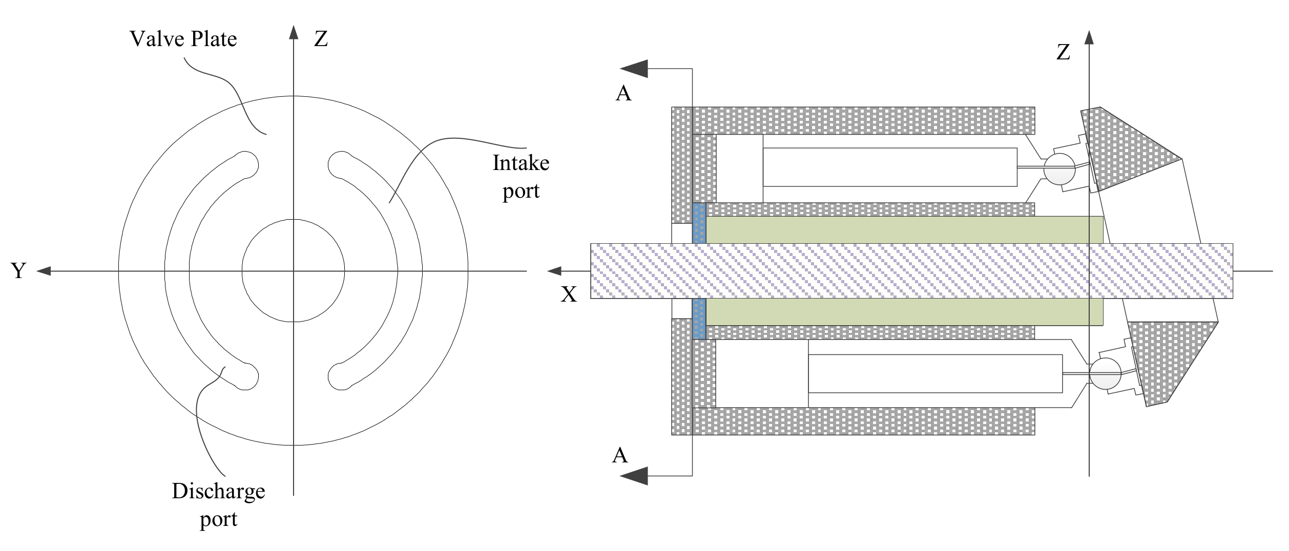
2. Introduction of ESPCS

The structural principle of the ESPCS studied herein is shown in Figure 3. Servo motor 1 axially drives the fixed-displacement pump. The suction and discharge ports of the fixed-displacement pump are connected to the two load ports of the hydraulic cylinder, and the fixed damping and electromagnetic switch valves are connected in series in the middle. The controller output a control command to the servo drive, and then control the speed of the servo motor, and then change the output flow of the fixed-displacement pump, adjust the displacement, speed, and output of the hydraulic cylinder. The replenishment circuit uses an accumulator and a one-way valve to replenish the system, and an electromagnetic switch valve was used to solve the flow asymmetry problem of the asymmetric cylinder in the ESPCS. The safety circuit uses an overflow valve to prevent pressure in the two chambers of the hydraulic cylinder. The ESPCS specifically includes a servo motor, a fixed-displacement pump, a hydraulic valve, an accumulator, a hydraulic cylinder, a servo drive, and a controller.

The system detects the actual position and pressure signal output from the hydraulic cylinder through the sensor and transmits it to the controller. Through the integrated processing of the pressure information, it outputs the speed control signal of the servo motor and then controls the output flow of the fixed-displacement pump to control the pressure change of the hydraulic cylinder. In this study, the fixed-displacement pump adopted an axial piston pump, and the servo motor used was a permanent magnet synchronous motor.

3. Mechanism Prediction Mathematical Model Establishment

3.1. Servo Motor Load–Speed Characteristic Mathematical Model

The servo motor is the core component of the system control as the execution terminal of the control algorithm.

The stator flux linkage equation of the servo motor is as follows:

$$\left\{\begin{array}{c}{\psi }_d=L_d{i}_d+{\psi }_f\\ {\psi }_q=L_q{i}_q\end{array}\right.$$

(1)

Servo motor stator voltage equation:

$$\left\{\begin{array}{l}{U}_d=R_s{i}_d+\frac{d}{dt}{\psi }_d-{\omega }_e{\psi }_q\hfill \\ U_q=R_s{i}_q+\frac{d}{dt}{\psi }_q+{\omega }_e{\psi }_d\hfill \end{array}\right.$$

(2)

Servo motor electromagnetic torque equation:

$$T_e=\frac{3}{2}{\delta }_n\left[{\psi }_f{i}_q+\left(L_d-L_q\right)i_d{i}_q\right]$$

(3)

Servo motor motion equation:

$$T_e-T_L=J_L\frac{d{\omega }_m}{dt}+D{\omega }_m$$

(4)

where ${\Psi }_d$, ${\Psi }_q$ are the d-q axis components of the stator flux linkage, $L_d$, $L_q$ are the d-q axis equivalent inductance of the stator inductances, $i_d$, $i_q$ are the d-q axis components of the stator current, ${\Psi }_f$ is the permanent magnet flux linkage, $U_d$, $U_q$ are the d-q axis components of the stator voltage, $R_s$ is the stator resistance, ${\omega }_e$ is the motor rotor angular speed, $T_e$ is the electromagnetic torque of the motor, ${\delta }_n$ is the number of pole pairs of the motor, $T_L$ is the load torque of the motor, $J_L$ is the equivalent converted moment of inertia of the rotor shaft, ${\omega }_m$ is the mechanical angular velocity of the motor, and $D$ is the damping coefficient of the motor.

3.2. Mathematical Model of Generalized Dead-Zone Characteristics of Fixed-Displacement Pump

The pump used herein was an axial plunger pump. According to the principle of the axial plunger pump, if an accurate model of the pump output flow is obtained, an accurate mathematical model must be established for each plunger suction and discharge process. Schematics of the working principle of the plunger pump and the single plunger oil discharge principle are shown in Figure 4 and Figure 5, respectively.

According to the Bernoulli equation, the classic orifice flow equation for a single plunger is derived as follows:

$$Q_n=sign(P_n-P_d)C_d{A}_o\sqrt{\frac{2}{\rho }\mid P_n-P_d\mid }$$

(5)

The flow generated by the multi-plunger of the fixed-displacement pump is as follows:

$$\stackrel{\wedge }{Q}=(\frac{\pi }{N{A}_p\tan (\alpha )w}){\displaystyle \sum _{n=1}^{n^{\prime }}sign(P_n-P_d)C_d{A}_o\sqrt{\frac{2}{\rho }\mid P_n-P_d\mid }}$$

(6)

where $A_p$ is the compression area of a single piston, $A_0$ is the cross-sectional flow discharge area for the nth piston chamber, $C_d$ is the flow coefficient, $N$ is the number of pistons in the pump body, $n^{\prime }$ is the number of plungers above the oil discharge port, $P_n$ is the pressure of the nth piston chamber, $P_d$ is the pressure of the oil outlet of the pump, $\widehat{Q}$ is the instantaneous flow of the fixed-displacement pump, $\rho$ is the fluid density, $w$ is the rotational angular velocity of the pump body, and $\alpha$ is the swash plate angle.

However, in the actual working process of the plunger pump, the cylinder body rotates at a high speed, and the oil between the cylinder body and the plunger is also in a fast-switching state of high and low pressure. In addition, owing to the manufacturing precision, there are inevitable leaks between each structural part; however, the amount of leakage has a positive correlation with the system pressure to a certain extent. Based on these factors, the fixed-displacement pump itself has a dead-zone characteristic of flow, and this dead-zone characteristic is mainly related to leakage, and we mainly analyze the leakage of the fixed-displacement pumps below. The internal leakage of the disc-type axial piston pump mainly occurs between the three main friction pairs; therefore, carrying out accurate modeling of the leakage model of the three friction pairs is necessary.

3.2.1. Shoe Pair Leakage Model

The leakage of the sliding shoe pair of the plunger pump can be regarded as the flow of the gap between the parallel disks. The oil flows through the center oil cavity of the sliding shoe and along the gap between the supporting surface of the swash plate, as shown in Figure 6.

As shown in Figure 6, the pressure difference flow is formed under the action of the pressure difference between the oil cavity pressure in the center of the shoe and the shell pressure. The relative movement between the shoe and the swash plate generates shear flow, but for the shear generated at this time, the flow will not affect the leakage of the shoe pair, and the leakage of the shoe swash plate can be expressed as:

$$Q_{L11}=\frac{\pi h^3(p_r-p_0)}{6\mu \ln \frac{r_2}{r_1}}$$

(7)

where $h$ is the oil film thickness between the stator and the slipper, $r_1$ is the inner radius of the slipper oil sealing belt, $r_2$ is the outer radius of the slipper oil sealing belt, $p_r$ is the slipper chamber pressure, and $p_0$ is the shell pressure.

3.2.2. Plunger Pair Leakage Model

The leakage model of the plunger pair is shown in Figure 5. The leakage flow rate of the plunger pair is expressed as:

$$Q_{L12}=\frac{\pi d{\delta }_1^3{P}_1}{12\mu L_1}(1+1.5{\epsilon }^3)$$

(8)

where $P_1$ is the pressure difference inside and outside the plunger cavity, $\mu$ is the dynamic viscosity of the oil, $L_1$ is the contact length between the plunger and the cylinder block, $d$ is the diameter of the plunger, ${\delta }_1$ is the gap between the plunger and the inner wall of the plunger hole of the rotor, and $\epsilon$ is the eccentricity.

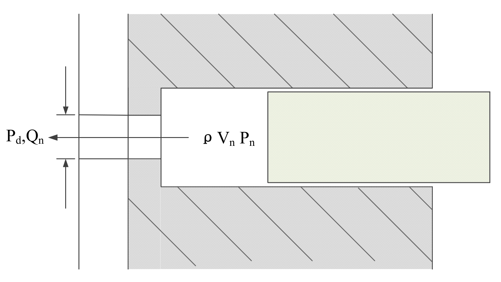
3.2.3. Port Flow Leakage Plate Model

Port flow leakage plate model is expressed as:

$$Q_{L13}=\frac{a{\delta }_3^3}{6\mu C_e}\left[\frac{1}{\ln (r_{12}/r_{11})}+\frac{1}{\ln (r_{14}/r_{13})}\right]P_3$$

(9)

where α is the covering angle of the valve plate waist groove, ${\delta }_3$ is the gap between the valve plate and the cylinder surface, $r_{12}$ is the pore size of the valve plate, $r_{11}$ is the inner radius of the valve plate waist groove, $r_{14}$ is the outer diameter of the valve plate, $r_{13}$ is the outer radius of the valve plate waist groove, $C_e$ is the flow coefficient of the valve plate, and $P_3$ is the pressure difference between the pores of the valve plate.

Therefore, the flow rate output by the pump port can be expressed as:

$$\begin{array}{ll}\stackrel{\wedge }{Q}=& (\frac{\pi }{N{A}_p\tan (\alpha )w}){\displaystyle \sum _{n=1}^{n^{\prime }}sign(P_n-P_d)C_d{A}_o}\sqrt{\frac{2}{\rho }\mid P_n-P_d\mid }-Q_{L11}-Q_{L12}-Q_{L13}\\ & =(\frac{\pi }{N{A}_p\tan (\alpha )w}){\displaystyle \sum _{n=1}^{n^{\prime }}sign(P_n-P_d)C_d{A}_o}\sqrt{\frac{2}{\rho }\mid P_n-P_d\mid }-\frac{\pi h^3(p_r-p_0)}{6\mu \ln \frac{r_2}{r_1}}-\\ & \left(\frac{\pi d{\delta }_1^3{P}_1}{12\mu L_1}(1+1.5{\epsilon }^3)\right)-\frac{a{\delta }_3^3}{6\mu C_e}\left[\frac{1}{\ln (r_{12}/r_{11})}+\frac{1}{\ln (r_{14}/r_{13})}\right]P_3\end{array}$$

(10)

3.3. Mathematical Model of Energy Storage Characteristics of Accumulator

In hydraulic systems, irregular pressure pulsation significantly affects the transmission performance of the hydraulic system, and pressure pulsation is widely present in hydraulic systems. The structure principle of the servo motor and axial piston pump changes the discharge flow with the internal operation of the pump body, i.e., there is a phenomenon of flow pulsation. Owing to the existence of liquid resistance, the flow pulsation will further evolve into pressure pulsation. Therefore, the source of the pressure pulsation is the flow pulsation. The flow pulsation phenomenon is more serious in the ESPCS under low-speed working conditions. When there is flow pulsation in the hydraulic system, the accumulator can absorb the peak flow in the hydraulic pipeline to compensate for the trough flow in the pipeline to reduce the flow pulsation, thereby effectively reducing the pressure pulsation in the pipeline. Therefore, an in-depth study of the energy storage characteristics of the accumulator is crucial for analyzing the nonlinear characteristics of the system flow. The mathematical model of the accumulator is established as follows:

To obtain an accurate description of the outlet flow of the accumulator, it is first necessary to accurately model the gas model pre-charged in the accumulator. A function diagram of the accumulator is shown in Figure 7.

The nonlinear model of the DDVC electro-hydraulic servo system has the characteristics of strong nonlinearity and many other characteristic parameters. Consequently, it is difficult to directly solve the problem. Therefore, it is necessary to linearize the nonlinear model of the system.

First, we provide the state equation of the ideal gas:

$$\frac{P_g{V}_g^k}{T}=R$$

(11)

where $P_g$ denotes the absolute pressure of the gas, $V_g$ is the volume of the gas, $k$ is the thermal insulation coefficient, $T$ is the thermodynamic temperature of the gas, and $R$ is the gas constant.

When the accumulator is used to absorb flow and pressure fluctuations, it can be understood as an adiabatic process. Therefore, the ideal gas state equation can be expressed as:

$$P_1{V}_1=P_2{V}_2=R$$

(12)

where $V_1$, $V_2$ are the instantaneous gas volumes at any two moments, and $P_1$, $P_2$ are the instantaneous gas pressures at any two moments.

According to Figure 7, we establish the force equation of the system.

$$(P_h-P_g)A=k_g\frac{V_g}{A}+C_g\frac{1}{A}\stackrel{.}{V_g}$$

(13)

where $k_g$ is the gas stiffness coefficient of the bladder at any time, and $C_g$ is the gas damping coefficient of the bladder at any time.

$$k_g=A^2\frac{dP}{dV}=A^2\frac{k{P}_g{V}_g^k}{V_g^{k+1}}$$

(14)

where $P_g$ is the instantaneous pressure of the gas in the accumulator and $V_g$ is the instantaneous volume of the gas in the accumulator.

$$C_g=8\pi {\mu }_g\frac{V_g}{A}$$

(15)

where ${\mu }_g$ is the gas viscosity coefficient.

The oil flow rate at the outlet end of the accumulator is $Q_S$, and the change in the oil flow rate at the outlet end is negatively related to the rate of change in the gas volume.

$$Q_s=-\stackrel{.}{V_g}=\frac{k_g{A}^3{P}_g{V}_g^{k+1}-(P_h-P_g)A{V}^{k+1}}{8\pi {\mu }_g{V}_g{V}^{k+1}}$$

(16)

3.4. Mathematical Model of Friction and Leakage Characteristics of Hydraulic Cylinder

To accurately describe the load flow of the hydraulic cylinder, we first need to accurately analyze the working principle of the hydraulic cylinder and subsequently establish an accurate mathematical model of the hydraulic cylinder. Although there are many types of existing hydraulic cylinders, their working principles are essentially the same. Based on the double-acting single-piston rod servo hydraulic cylinder, this study establishes a dynamic model. A schematic of its working principle is shown in Figure 8.

Taking the piston moving to the right as an example, the flow equation of the rodless cavity and rod cavity of the hydraulic cylinder can be expressed as

$$Q_{L8i}=V_1+C_{ip}(p_1-p_2)+(V_1/{\beta }_e)p_1$$

(17)

$$Q_{L8o}=-V_2+C_{ip}(p_1-p_2)-C_{ep}{p}_2-(V_2/{\beta }_e)p_2$$

(18)

where $V_1$ is the volume of the rodless cavity ($V_1=V_{10+}{A}_{1}y$), $V_2$ is the rod cavity volume, $y$ is the piston displacement, $V_{10}$ is the initial volume of the rodless cavity oil, $V_{20}$ is the initial volume of oil with rod cavity, $C_{ip}$ is is the internal leakage coefficient of the hydraulic cylinder, $C_{ep}$ is is the external leakage coefficient of the hydraulic cylinder, and ${\beta }_e$ is the effective volumetric elastic modulus of hydraulic oil.

According to the definition of load traffic $Q_L=Q_{L8i}$, the load traffic can be deduced:

$$Q_L=A_{1}y-C_{sp}{p}_s+C_{tp}{p}_L+V_e{p}_L/4{\beta }_e$$

(19)

where $C_{sp}$ is the additional leakage factor ($C_{sp}=\left(1-n\right)C_{ip}/\left(1+n\right)$), $C_{tp}$ is the equivalent leakage coefficient ($C_{tp}=2C_{ip}/\left(1+n\right)$), $V_e$ is the equivalent volume ($V_{10}=4V_1/\left(1+n\right)$); generally, the equivalent volume is the volume when the piston is in the middle position, $V_e=2\left(2V_0+A_{1}L\right)/\left(1+n\right)$, $L$ is the stroke of the piston.

$$Q_{L8i}=C_{ip}(p_1-p_2)+C_{ep}{p}_1+\frac{V_1}{{\beta }_e}\frac{d{p}_1}{dt}+A_1\frac{dy}{dt}$$

(20)

$$Q_{L8o}=C_{ip}(p_1-p_2)-C_{ep}{p}_2-\frac{V_2}{{\beta }_e}\frac{d{p}_2}{dt}+A_2\frac{dy}{dt}$$

(21)

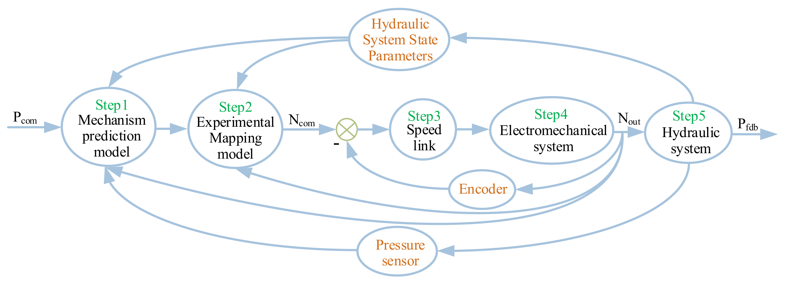
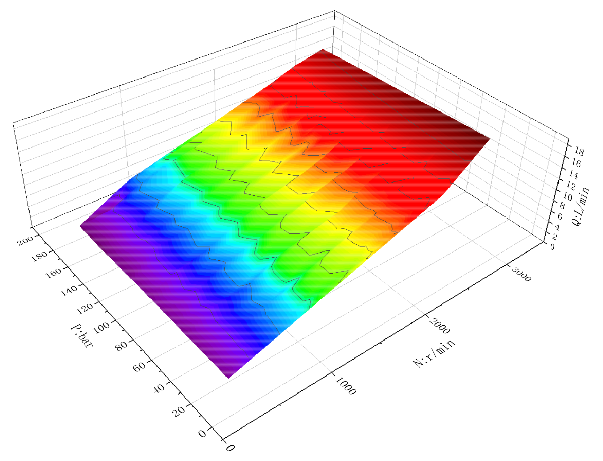
3.5. Flow Mechanism Prediction Model of Electrohydraulic Servo Pump-Control System

We established a mechanism prediction model for the core components of the system. Based on the schematic shown in Figure 9, we need to build a mechanism prediction model for the entire system.

According to the flow characteristics of the small hole, Equation (22) is obtained.

$$\left\{\begin{array}{l}{Q}_{s1}=C_{ds1}{A}_{s1}\sqrt{\frac{2}{\rho }(P_1-P_L)}\\ Q_{o1}=C_{do1}{A}_{o1}\sqrt{\frac{2}{\rho }(P_2-P_1)}\\ Q_{o2}=-C_{d02}{A}_{02}\sqrt{\frac{2}{\rho }(P_3-P_4)}\end{array}\right.$$

(22)

According to the flow continuity equation, Equation (23) is obtained.

$$\left\{\begin{array}{l}{Q}_o-Q_{s1}-Q_{s2}=\frac{d{V}_1}{dt}+\frac{V_1}{{\mathsf{\beta }}_e}\frac{d{P}_1}{dt}\\ Q_{o1}-Q_{s3}-Q_{L8}=\frac{d{V}_2}{dt}+\frac{V_2}{{\mathsf{\beta }}_e}\frac{d{P}_2}{dt}\\ Q_{L8}-Q_{o2}-Q_{s6}=\frac{d{V}_3}{dt}+\frac{V_3}{{\mathsf{\beta }}_e}\frac{d{P}_3}{dt}\\ Q_{o2}-Q_{s5}=\frac{d{V}_4}{dt}+\frac{V_4}{{\mathsf{\beta }}_e}\frac{d{P}_4}{dt}\end{array}\right.$$

(23)

$V_1$, $V_2$, $V_3$, $V_4$ can also be defined in the form shown in Equation (24).

$$\left\{\begin{array}{l}{V}_1=V_{10}+A_1{y}_1\\ V_2=V_{20}+A_{R1}y+A_2{y}_2\\ V_3=V_{30}-A_{R2}y+A_6{y}_6\\ V_4=V_{40}+A_5{y}_5\end{array}\right.$$

(24)

Now let us define the state of the system as:

$$x_1=y,x_2=\stackrel{.}{y},x_3=P_1,x_4=P_2,x_5=P_3,x_6=P_4$$

The equation of state for the whole system is:

$$\left\{\begin{array}{l}\stackrel{.}{x_1}=x_2\\ \stackrel{.}{x_2}=\frac{A_{R1}{x}_4-A_{R2}{x}_5-C{x}_2-K{x}_1-F}{m}\\ \stackrel{.}{x_3}=\frac{Q_o-Q_{s1}-Q_{s2}-A_1{V}_1}{(V_{10}+A_1{y}_1)/{\mathsf{\beta }}_e}\\ \stackrel{.}{x_4}=\frac{Q_{o1}-Q_{s3}-Q_{L8}-A_2{V}_2-A_{R1}{x}_2}{(V_{20}+A_{R1}{x}_1+A_2{y}_2)/{\mathsf{\beta }}_e}\\ \stackrel{.}{x_5}=\frac{Q_{L8}+Q_{o2}-Q_{s6}-A_6{V}_6-A_{R2}{x}_2}{(V_{40}+A_5{y}_5)/{\mathsf{\beta }}_e}\end{array}\right.$$

(25)

4. Experimental Study

We herein explore the influence of the nonlinear characteristics of the various components of the ESPCS on the nonlinear characteristics of the system flow, as well as the influence of the coupling characteristics between the system components on the system pressure control. We conducted experimental research on the strong nonlinearity in the system, such as the load–speed characteristics of the servo motor, generalized dead-zone characteristics of the hydraulic pump, energy storage characteristics of the accumulator, and the friction characteristics of the hydraulic cylinder, and subsequently obtained the corresponding mapping model. Finally, the experimental research on the pressure control accuracy based on the nonlinear flow prediction and mapping model is carried out, and it is verified that the model can significantly improve the pressure control accuracy.

4.1. Experimental Research Conditions

Based on the experimental platform of pump-controlled hydraulic actuators, we herein conducted experimental research on the nonlinear characteristics of the system flow. The hydraulic experiment platform included motor pump units, functional valve blocks, and hydraulic cylinders. The electrically integrated cabinet includes electrical components such as axis controllers and servo drives. The mechanism prediction model and experimental mapping mathematical model can be imported into the axis controller using MATLAB. The composition of the experimental platform is shown in Figure 10.

4.2. Experimental Curve Analysis and Research

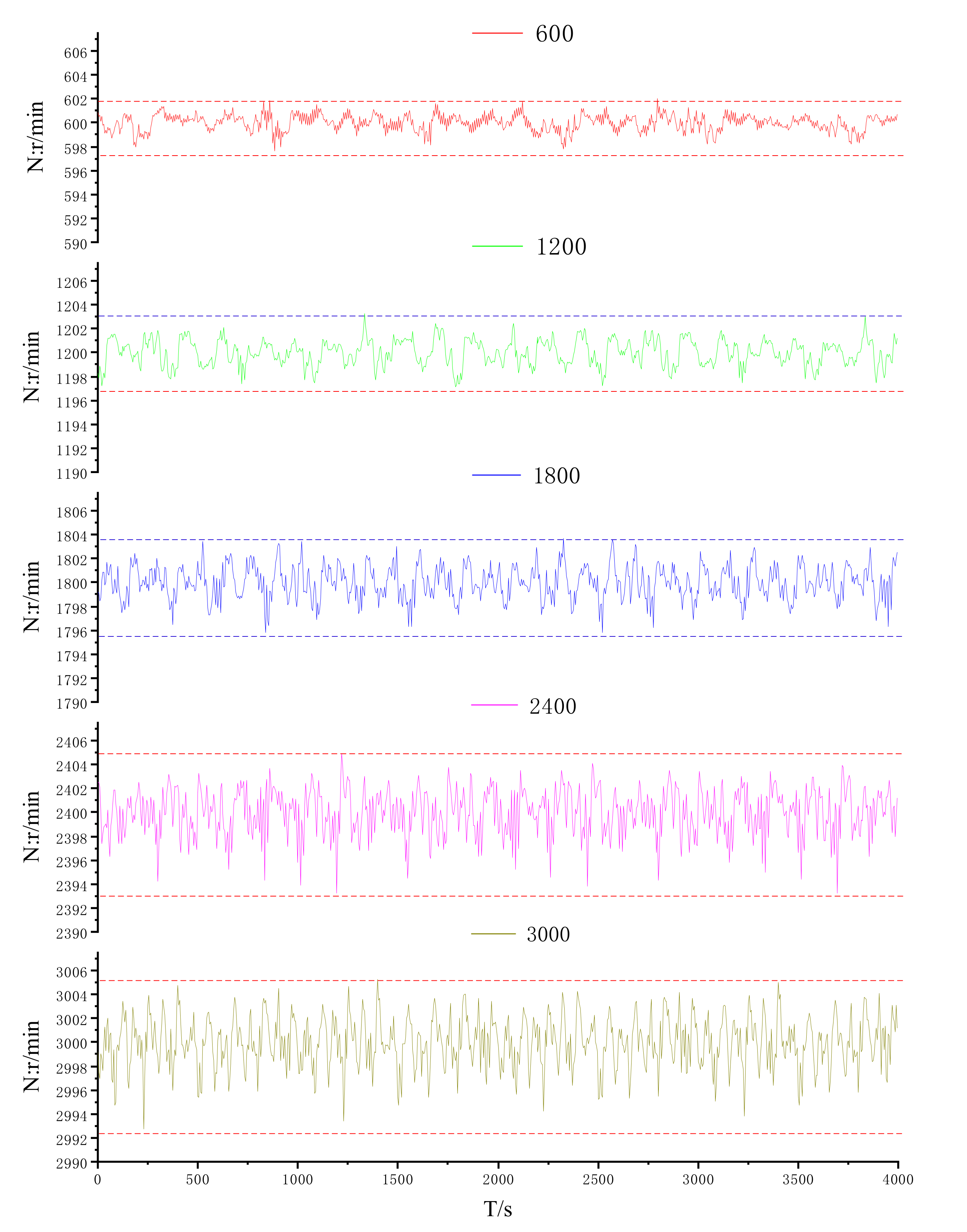
4.2.1. Experimental Study on Load–Speed Characteristics of Servo Motor

In the actual control process, the coincidence degree between the actual speed and the target speed of the servo motor will affect the control precision of the system to a great extent. There are two main factors causing the fluctuation of servo motor speed: on the one hand, the fluctuation of servo motor speed will be significantly different under different speeds. On the other hand, the disturbance of external load will also cause the fluctuation of servo motor speed. These two factors are difficult to express by means of microscopic mechanism modeling at present. So, we established the experimental mapping model of servo motor speed fluctuation through two groups of experiments.

First, at a constant speed, the fluctuation of the servo motor speed under different loads was obtained by adjusting the load sizes, as shown in Figure 11.

According to the experimental data in Figure 11, the speed fluctuation of the servo motor is shown to be positively correlated with the load and approximately linear. We define the speed fluctuation of the servo motor as $V_{volatility}$, and we then establish the linear mapping equation of the speed fluctuation of the servo motor and the load as follows.

$$V_{volatility}=K_l{F}_{load}$$

(26)

where $K_l$ is the correlation coefficient of speed, and $F_{load}$ is the servo motor shaft-end load.

In addition, at a constant pressure of 6 MPa, we obtained the fluctuation of the servo motor speed at different speeds by adjusting the speed, as shown in Figure 12.

According to the above experimental data, the fluctuation of the servo motor speed also positively correlated with that of the speed, which can also be approximated as a linear relation. Therefore, we establish the linear mapping equation of the servo motor speed fluctuation and speed as follows.

$$V_{volatility}=K_a{V}_{actual}$$

(27)

where $K_a$ is the servo motor speed correlation coefficient and $V_{actual}$ is the servo motor shaft-end speed.

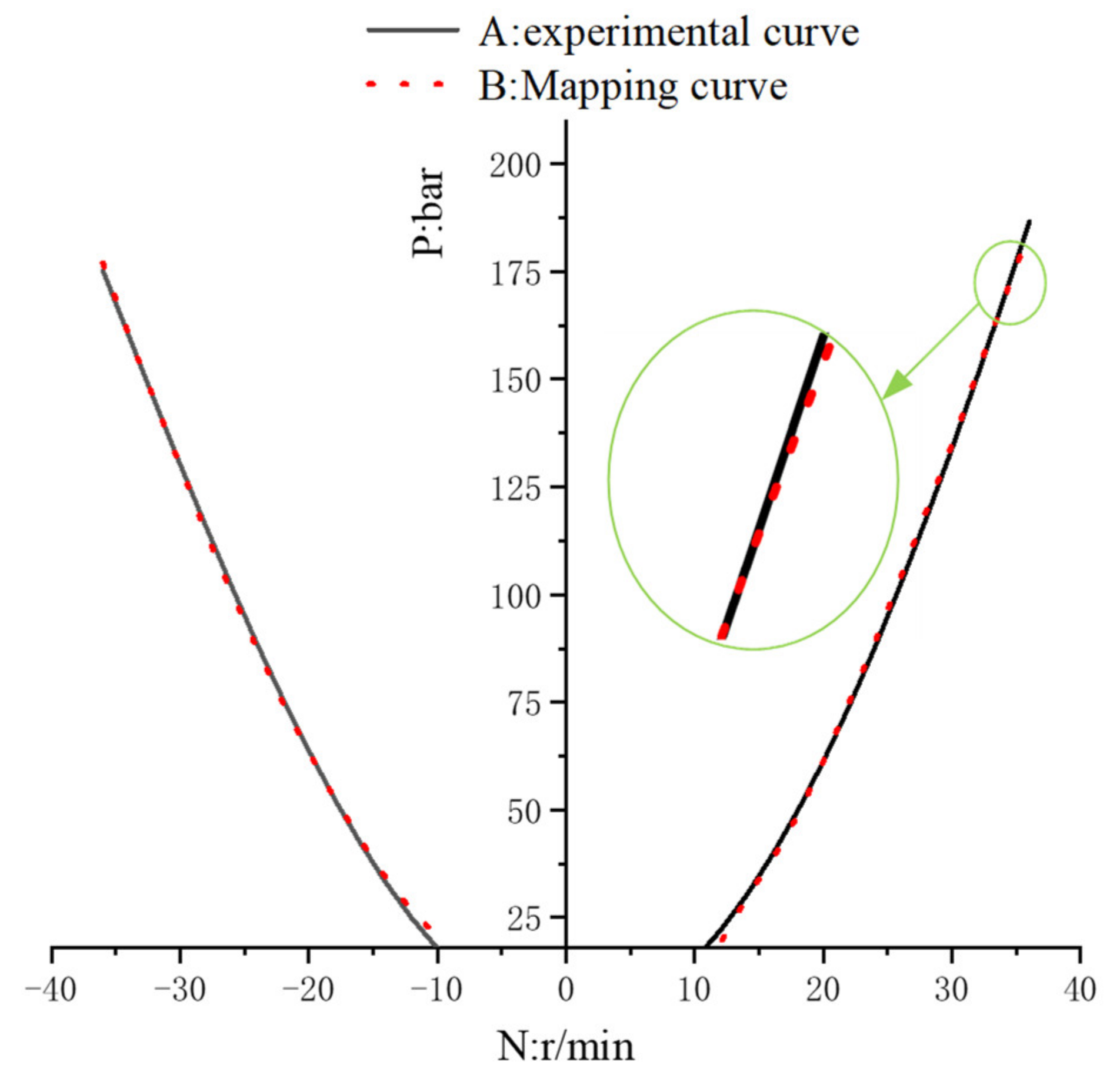
4.2.2. Experimental Study on Generalized Dead-Zone Characteristics of Fixed-Displacement Pump

A fixed-displacement pump is a direct output flow element of the hydraulic system, and the output flow is extremely nonlinear. From the perspective of high-precision control, the factors that affect the control accuracy mainly include the dead zone of the fixed-displacement pump and the flow attenuation of the fixed-displacement pump. From a broad perspective, the attenuation of the output flow of the fixed-displacement pump can be seen as a result of the dead zone of the fixed-displacement pump flow, and the role of the dead zone exists anytime and anywhere. Therefore, we conducted a generalized dead-zone experimental study for this aspect.

First, we carried out a system-pressure building experiment using a fixed-displacement pump at low speed. A schematic of the experimental principle is shown in Figure 13.

In Figure 13, 3.1, and 3.2 record the inlet and outlet pressure of the fixed-displacement pump; 5.1 and 5.1 work with accumulators to compensate the oil in the system when the experimental conditions need to be revised; 4.2 and 4.3 need to be opened for system unloading to ensure consistency of the initial pressure of the system; and 7.1 and 7.2 measure the output flow of the pump. Next, we pump A cavity through the electromagnetic directional valve closed 4.1, increasing speed, record the maximum pressure that can be achieved in chamber A of the fixed-displacement pump; when the system pressure remains unchanged, the internal leakage of the fixed-displacement pump to provide a fixed-displacement pump, and the compression of the oil; under different rotational speeds, the pressure of the experimental data is recorded, and the same operation is performed when the pump is reversed. The experimental results are shown in Figure 14.

To accurately express the dead zone and effectively compensate for the dead zone effect, accurately characterizing the phenomenon caused by the dead-zone effect is necessary. Through the analysis of the experimental data, we applied a Gaussian function to fit the experimental data and obtained the following Equation (28). The fitting effect of the experimental data is shown in Figure 15. From this, we also obtained an accurate mapping mathematical model of the dead-zone effect. The parameter values of Formula 28 can be found in the Appendix A.

$$\begin{array}{ll}f(x)=& a_{11}\exp (-{((x-b_{11})/c_{11})}^2)+a_{12}\exp (-{((x-b_{12})/c_{12})}^2)+\\ & a_{13}\exp (-{((x-b_{13})/c_{13})}^2)+a_{14}\exp (-{((x-b_{14})/c_{14})}^2)+\\ & a_{15}\exp (-{((x-b_{15})/c_{15})}^2)+a_{16}\exp (-{((x-b_{16})/c_{16})}^2)\end{array}$$

(28)

Given the attenuation problem of the fixed-displacement pump flow, we measured the experimental data of the system output flow under different speeds and pressures, as shown in Figure 16.

The experimental data shows that if we accurately describe the envelope surface of the output flow of the hydraulic pump, then we can perfectly provide real-time and accurate flow mapping compensation for high-precision control. Next, we express the output flow envelope surface of the hydraulic pump obtained from the experiment through a third-order polynomial, as shown in Equation (29), and the envelope surface of the mapping mathematical model is shown in Figure 17. From this, we obtain a mapping model of the output flow of the hydraulic pump. The parameter values of Formula 29 can be found in the Appendix A.

$$\begin{array}{ll}f(x,y)=& p_{00}+p_{10}x+p_{01}y+p_{20}{x}^2+p_{11}xy+p_{02}{y}^2+\\ & p_{30}{x}^3+p_{21}{x}^{2}y+p_{12}x{y}^2+p_{03}{y}^3\end{array}$$

(29)

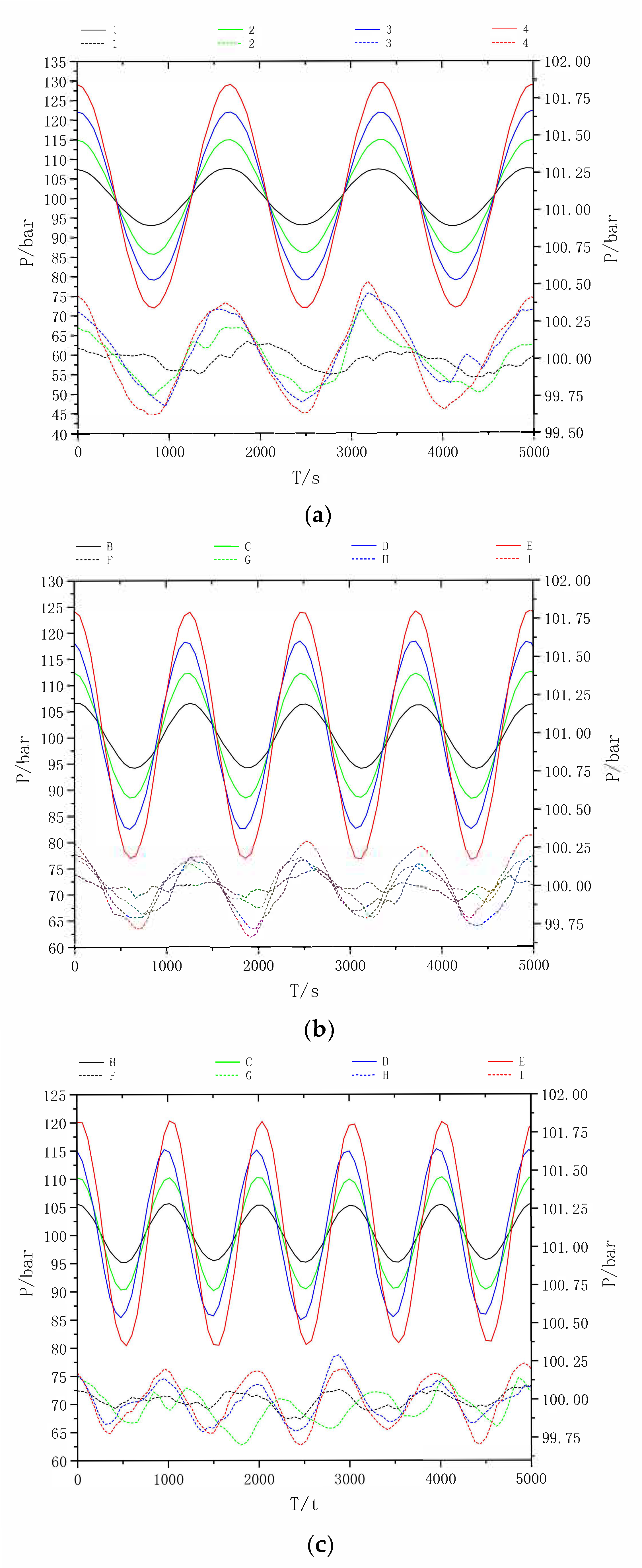
4.2.3. Experimental Study on Accumulator Energy Storage Characteristics

The accumulator is the key component of a system that absorbs pressure fluctuations. To obtain the performance of the accumulator to absorb pressure fluctuations, we simulated pressure fluctuations of different amplitudes and frequencies. Under the same inflation pressure, the accumulator’s ability to absorb different amplitudes and frequencies was experimentally studied. The hydraulic principle is shown in Figure 18. We adjust the opening size of the throttle valve 7, and by setting the sinusoidal speed signal of the servo motor (the sinusoidal speed here, the direction of the speed is not allowed to change), the flow exhibits sinusoidal fluctuations owing to the existence of damping, and the pressure also presents sinusoidal fluctuations. A control experiment for the accumulator to absorb pressure fluctuations was obtained by controlling the on and off switch of the solenoid valve 4.3. The experimental data are shown in Figure 19.

In Figure 19, the pressure fluctuation frequencies of the three experimental groups from left to right are 0.6 Hz, 0.8 Hz, and 1 Hz. The experimental results show that under the same charging pressure, the accumulator has a significant effect on the absorption capacity of high-frequency pressure fluctuations but not on the absorption capacity of low-frequency pressure fluctuations.

4.2.4. Experimental Study on the Friction Characteristics of Hydraulic Cylinder

We built a pump-controlled hydraulic cylinder friction characteristics test bench to accurately describe the friction characteristics of a hydraulic cylinder. The hydraulic principle is shown in Figure 20. Given the servo motor speed sinusoidal signal, the output flow of the fixed-displacement pump shows sinusoidal periodic changes, and it then drives the reciprocating motion of the hydraulic cylinder. The data of the hydraulic cylinder inlet and outlet pressure, hydraulic cylinder displacement, hydraulic cylinder acceleration, and hydraulic cylinder speed are shown in Figure 21 and Figure 22, respectively, and the data curve of the friction force of the hydraulic cylinder is obtained through the force equation of the hydraulic cylinder. The curve of hydraulic cylinder friction varying with velocity is shown in Figure 23.

The pressure signals of the two cavities of the hydraulic cylinder are collected by the sine speed instruction of the servo motor, and the position information of the hydraulic cylinder is also collected by the external displacement sensor

By collecting and processing the displacement information of the hydraulic cylinder, the real-time velocity and acceleration of the hydraulic cylinder are obtained respectively.

The Fourier equation is used to express the friction characteristics, and the mathematical expression of the friction force of the cylinder and the cylinder speed with the time-independent variable is obtained as the mapping mathematical model of the friction and velocity of the hydraulic cylinder. Figure 24 shows the fitting effect between the mapping model and actual friction characteristics.

Mathematical model of cylinder friction mapping:

$$\begin{array}{ll}{f}_{friction}\left(x\right)=& a_{00}+a_{21}\cos \left(x{w}_1\right)+b_{21}\sin \left(x{w}_1\right)+a_{22}\cos \left(2x{w}_1\right)+\\ & b_{22}\sin \left(2x{w}_1\right)+a_{23}\cos \left(3x{w}_1\right)+b_{23}\sin \left(3x{w}_1\right)+\\ & a_{24}\cos \left(4x{w}_1\right)+b_{24}\sin \left(4x{w}_1\right)+a_{25}\cos \left(5x{w}_1\right)+\\ & b_{25}\sin \left(5x{w}_1\right)\end{array}$$

(30)

The parameter values of Formula 30 can be found in the Appendix A.

Cylinder velocity mapping mathematical model:

$$\begin{array}{cc}{f}_{velocity}\left(x\right)=\hfill & a_{01}+a_{31}\cos \left(x{w}_2\right)+b_{31}\sin \left(x{w}_2\right)+a_{33}\cos \left(2x{w}_2\right)+\\ & b_{32}\sin \left(2x{w}_2\right)+a_{33}\cos \left(3x{w}_2\right)+b_{33}\sin \left(x{w}_2\right)+\hfill \\ & a_{34}\cos \left(4,x,w_2\right)+b_{34}\sin \left(4x{w}_2\right)+a_{35}\cos \left(5x{w}_2\right)+\hfill \\ & b_{35}\sin \left(5x{w}_2\right)+a_{36}\cos \left(6x{w}_2\right)b_{36}\sin \left(6x{w}_2\right)+\hfill \\ & a_{37}\cos \left(7x{w}_2\right)+b_{37}\sin \left(7x{w}_2\right)+a_{38}\cos \left(8x{w}_2\right)+\hfill \\ & b_{38}\sin \left(8x{w}_2\right)\hfill \end{array}$$

(31)

The mapping of Equations (31) and (32) express the functional relation between the friction force of the hydraulic cylinder and the speed simultaneously. Subsequently, with time as the link, we link the friction of the cylinder with the speed.

Fourier formula was used to fit the experimental data, and the fitting effect was shown in Figure 24.

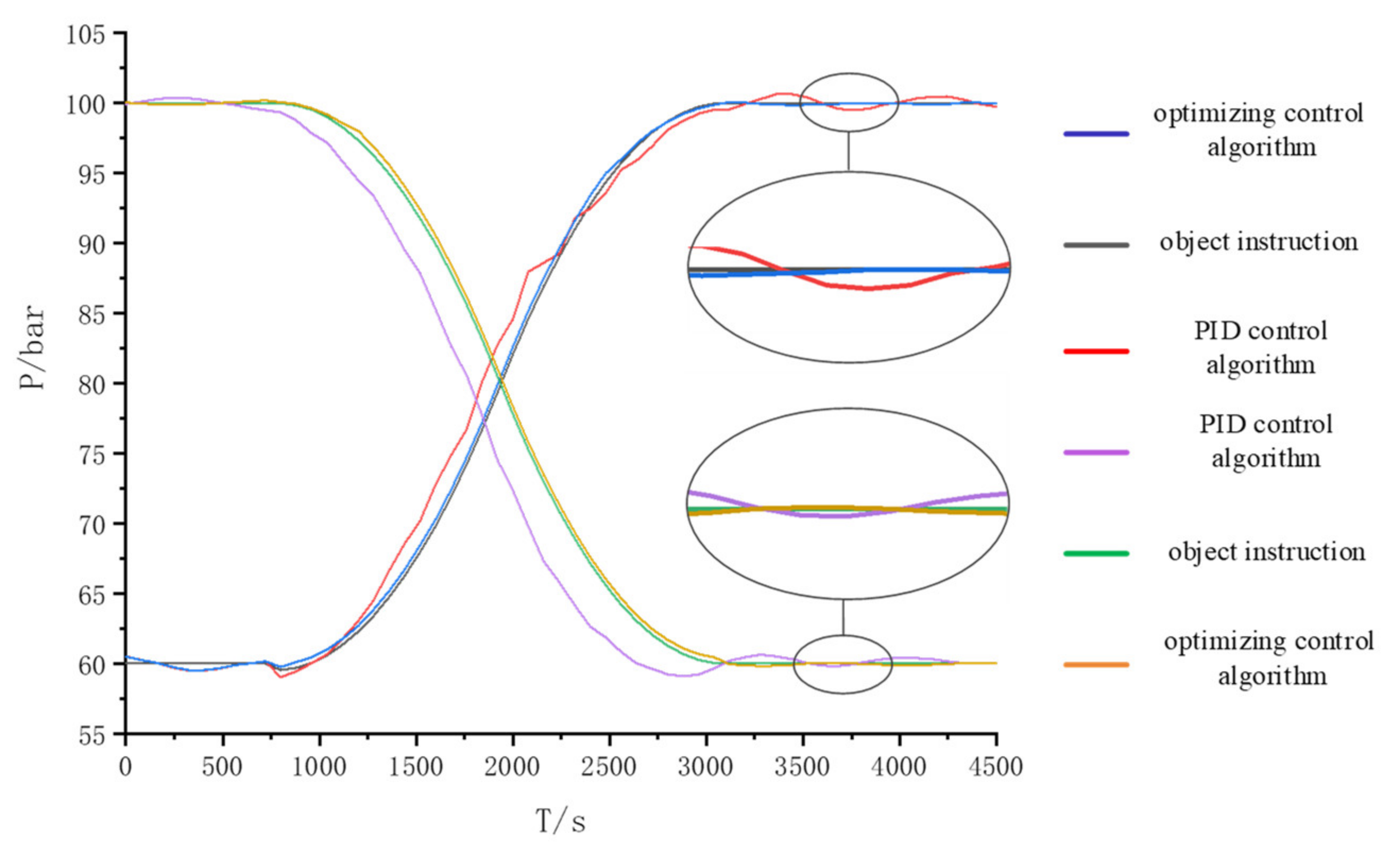
4.2.5. Experimental Verification of High-Precision Pressure Control Based on Flow Nonlinear Compensation

The system mechanism prediction model was integrated with the experimental mapping mathematical model using MATLAB, and the control algorithm was downloaded to the system axis controller using the MACS software to achieve real-time pressure control of the test platform.

The accuracy of the pressure control was compared using two sets of experiments. One set is a pressure control experiment using a compound control algorithm that combines a mechanism prediction model and an experimental mapping model. Another group set up a PID control algorithm to perform a control experiment. The experimental results are shown in Figure 25.

Through the given pressure instructions, the traditional PID algorithm and the optimized algorithm are respectively used for experiments. The experimental results show that the method adopted herein has considerably improved the accuracy of pressure following compared with the PID control algorithm. There was no overshoot phenomenon. The accuracy of the PID control algorithm is ±0.12 MPa. The test accuracy of the method used in this study was 0.037 MPa, and the steady-state control accuracy greatly improved.

5. Conclusions

To improve the pressure control accuracy of the ESPCS, in this study, we use a combination of a mechanism prediction model and an experimental mapping model to accurately describe the flow nonlinear phenomenon in the ESPCS and achieve accurate and fast tracking of the target trajectory. The steady-state pressure control accuracy of the system was considerably improved. In addition, in this paper, the relation between the dead zone of the hydraulic pump, flow attenuation of the full speed range, friction of the hydraulic cylinder and the speed, through experimental research, has obtained an accurate mapping mathematical model. We have ensured that the control algorithm accurately compensates for nonlinear phenomena in the system. A comparison with the traditional PID control algorithm shows that the method used herein to improve the pressure control accuracy can significantly increase the pressure control accuracy. The results of this study have broad application prospects in the fields of hydraulic quadruped robots and high-precision pressure control military industry in the future. However, our research also had shortcomings. It fails to express the relation between the accumulator’s energy storage characteristics and its charging pressure and system pressure fluctuation characteristics with an accurate mapping mathematical model. In future follow-up research, we will rebuild a set of experimental platforms, to conduct a comprehensive experimental study on the energy storage characteristics of the accumulator. Finally, a more accurate experimental mapping model is obtained.

References

1. Luo, G.; Görges, D. Modeling and Adaptive Robust Force Control of a Pump-Controlled Electro-Hydraulic Actuator for an Active Suspension System. In Proceedings of the 2019 IEEE Conference on Control Technology and Applications (CCTA), Hong Kong, China, 19–21 August 2019; pp. 592–597. [Google Scholar]
2. Li, X.; Jiao, Z.; Yan, L.; Cao, Y. Modeling and Experimental Study on a Novel Linear Electromagnetic Collaborative Rectification Pump. Sens. Actuators A Phys. 2020, 309, 111883. [Google Scholar] [CrossRef]
3. Lee, S.R.; Hong, Y.S. A Dual EHA System for the Improvement of Position Control Performance Via Active Load Compensation. Int. J. Precis. Eng. Manuf. 2017, 18, 937–944. [Google Scholar] [CrossRef]
4. Yuan, H.B.; Na, H.C.; Kim, Y.B. Robust MPC–PIC force control for an electro-hydraulic servo system with pure compressive elastic load. Control Eng. Pract. 2018, 79, 170–184. [Google Scholar] [CrossRef]
5. Zhu, Y.; Jiang, W.L.; Kong, X.D.; Zheng, Z. Study on nonlinear dynamics characteristics of electrohydraulic servo system. Nonlinear Dyn. 2015, 80, 723–737. [Google Scholar] [CrossRef]
6. Hao, Y.; Xia, L.; Ge, L.; Wang, X.; Qvan, L. Research on Position Control Characteristics of Hybrid Linear Drive System. Trans. Chin. Soc. Agric. Mach. 2020, 51, 379–385. [Google Scholar]
7. Jing, C.; Xu, H.; Jiang, J. Dynamic surface disturbance rejection control for electro-hydraulic load simulator. Mech. Syst. Signal Process. 2019, 134, 106293. [Google Scholar] [CrossRef]
8. Zhang, L.; Guo, F.; Li, Y.; Lu, W. Global dynamic modeling of electro-hydraulic 3-UPS/S parallel stabilized platform by bond graph. Chin. J. Mech. Eng. 2016, 29, 1176–1185. [Google Scholar] [CrossRef]
9. Yu, Z.; Leng, B.; Xiong, L.; Feng, Y.; Shi, F. Direct yaw moment control for distributed drive electric vehicle handling performance improvement. Chin. J. Mech. Eng. 2016, 29, 486–497. [Google Scholar] [CrossRef]
10. Wang, C.; Quan, L. Characteristic of Pump Controlled Single Rod Cylinder with Combination of Variable Displacement and Speed. Trans. Chin. Soc. Agric. Mach. 2017, 48, 405–412. [Google Scholar]
11. Yue, J.; Dai, B.; Xu, W.U.; Yang, L. The Impact of Flow Pulsation of Axial Piston Pump on Gun Pitching Accuracy of a Multiple Rocket Launcher. Acta Armamentarii 2019, 40, 1781. [Google Scholar]
12. Wang, L.; Wang, D.; Qi, J.; Xue, Y. Internal leakage detection of hydraulic cylinder based on wavelet analysis and backpropagation neural network. In Proceedings of the 2020 Global Reliability and Prognostics and Health Management (PHM-Shanghai), Shanghai, China, 16–18 October 2020; pp. 1–6. [Google Scholar]
13. Li, Y.; Shang, Y.; Jiao, Z. EHA position system simulation based on fuzzy sliding mode control. In Proceedings of the CSAA/IET International Conference on Aircraft Utility Systems (AUS 2018), Guiyang, China, 19–22 June 2018; pp. 1012–1016. [Google Scholar] [CrossRef]
14. Xia, H.; Yang, B.; Shang, Y.; Jiao, Z. Simulation and verification of pressure characteristics of aircraft hydraulic power system. In Proceedings of the 2019 IEEE 8th International Conference on Fluid Power and Mechatronics (FPM), Wuhan, China, 10–13 April 2019; pp. 1197–1202. [Google Scholar]
15. Li, J.; Fu, Y.; Zhang, G.; Gao, B.; Ma, J. Research on fast response and high accuracy control of an airborne brushless DC motor. In Proceedings of the IEEE International Conference on Robotics & Biomimetics, Shenyang, China, 22–26 August 2004; pp. 807–810. [Google Scholar]
16. Guo, J.; Ye, C.; Wu, G. Simulation and Research on Position Servo Control System of Opposite Vertex Hydraulic Cylinder based on Fuzzy Neural Network. In Proceedings of the 2019 IEEE International Conference on Mechatronics and Automation (ICMA), Tianjin, China, 4–7 August 2019; pp. 1139–1143. [Google Scholar]
17. Essa, M.E.S.M.; Aboelela, M.A.; Hassan, M.M.; Abdraboo, S.M. Fractional order fuzzy logic position and force control of experimental electro-hydraulic servo system. In Proceedings of the 2019 8th International Conference on Modern Circuits and Systems Technologies (MOCAST), Thessaloniki, Greece, 13–15 May 2019; pp. 1–4. [Google Scholar]
18. Essa ME, S.M.; Aboelela, M.A.; Hassan, M.M.; Abdrabbo, S.M. Control of hardware implementation of hydraulic servo application based on adaptive neuro fuzzy inference system. In Proceedings of the 2018 14th International Computer Engineering Conference (ICENCO), Cairo, Egypt, 29–30 December 2018; pp. 168–173. [Google Scholar]
19. Milić, V.; Šitum, Ž.; Essert, M. Robust position control synthesis of an electro-hydraulic servo system. ISA Trans. 2010, 49, 535–542. [Google Scholar] [CrossRef] [PubMed]
20. Yin, X.; Zhang, W.; Jiang, Z.; Pan, L. Adaptive robust integral sliding mode pitch angle control of an electro-hydraulic servo pitch system for wind turbine. Mech. Syst. Signal Process. 2019, 133, 105704. [Google Scholar] [CrossRef]
21. Xu, G.; Chen, M.; He, X.; Pang, H.; Miao, H.; Cui, P.; Wang, W.; Diao, P. Path following control of tractor with an electro-hydraulic coupling steering system: Layered multi-loop robust control architecture. Biosyst. Eng. 2021, 209, 282–299. [Google Scholar] [CrossRef]
22. Lin, Y.; Shi, Y.; Burton, R. Modeling and robust discrete-time sliding-mode control design for a fluid power electrohydraulic actuator (EHA) system. IEEE/ASME Trans. Mechatron. 2011, 18, 1–10. [Google Scholar] [CrossRef]
23. Zhang, H.; Liu, X.; Wang, J.; Karimi, H.R. Robust H∞ sliding mode control with pole placement for a fluid power electrohydraulic actuator (EHA) system. Int. J. Adv. Manuf. Technol. 2014, 73, 1095–1104. [Google Scholar] [CrossRef] [Green Version]
24. Kim, H.M.; Park, S.H.; Song, J.H.; Kim, J.S. Robust position control of electro-hydraulic actuator systems using the adaptive back-stepping control scheme. Proc. Inst. Mech. Eng. 2010, 224, 737–746. [Google Scholar] [CrossRef]
25. Ahn, K.K.; Nam, D.N.C.; Jin, M. Adaptive Backstepping Control of an Electrohydraulic Actuator. IEEE/ASME Trans. Mechatron. 2013, 19, 987–995. [Google Scholar] [CrossRef]
26. Shen, Y.; Wang, X.; Wang, S.; Mattila, J. An Adaptive Control Method for Electro-hydrostatic Actuator Based on Virtual Decomposition Control. In Proceedings of the 2020 Asia-Pacific International Symposium on Advanced Reliability and Maintenance Modeling (APARM), Vancouver, BC, Canada, 20–23 August 2020; pp. 1–6. [Google Scholar]
Figure 1. Schematic of servo pump-controlled energy transfer.
Processes 10 00786 g001
Figure 2. ESPCS pressure control chart.
Processes 10 00786 g002
Figure 3. Schematic of the ESPCS structure: 1—servo motor; 2—fixed-displacement pump; 3—low pressure pressure sensor; 4.1/4.2/4.3/4.4/4.5—accumulator; 5.1/5.2/5.3/5.4—solenoid switch valve; 6.1/6.2—safety relief valve; 7.1/7.2—check valve; 8.1/8.2/8.3/8.4—high pressure sensor; 9—hydraulic cylinder; 10—displacement sensor; 11—controller; 12—servo driver; 13.1/13.2—hydraulic damping.
Processes 10 00786 g003
Figure 4. Schematic of the working principle of the plunger pump.
Processes 10 00786 g004
Figure 5. Schematic of single plunger oil discharge principle.
Processes 10 00786 g005
Figure 6. Sketch of the pair of skates.
Processes 10 00786 g006
Figure 7. Function diagram of the accumulator.
Processes 10 00786 g007
Figure 8. Schematic of hydraulic cylinder.
Processes 10 00786 g008
Figure 9. Schematic of ESPCS.
Processes 10 00786 g009
Figure 10. Schematic of the experimental platform. (a) Control system test platform; (b) hydraulic electrical system test platform.
Processes 10 00786 g010
Figure 11. Fluctuation of servo motor speed (constant speed/variable load).
Processes 10 00786 g011
Figure 12. Fluctuation of servo motor speed (constant load/variable speed).
Processes 10 00786 g012
Figure 13. Schematic of the dead-zone compression test. 1—servo motor; 2—fixed-displacement pump; 3.1/3.2—pressure gage; 4.1/4.2/4.3—magnetic exchange valve; 5.1/5.2—one-way valve; 6—accumulator; 7.1/7.2—flow sensor.
Processes 10 00786 g013
Figure 14. Dead-zone construction pressure curve.
Processes 10 00786 g014
Figure 15. Dead-zone build pressure mapping.
Processes 10 00786 g015
Figure 16. Experimental diagram of pump flow envelope surface.
Processes 10 00786 g016
Figure 17. Pump flow mapping.
Processes 10 00786 g017
Figure 18. Schematic of accumulator experiment exploration. 1—servo motor; 2—fixed-displacement pump; 3.1/3.2—pressure gage; 4.1/4.2/4.3—magnetic exchange valve; 5.1/5.2—one-way valve; 6.1/6.2—accumulator; 7—throttling valve; 7.1/7.2—flow sensor.
Processes 10 00786 g018
Figure 19. Schematic of accumulator experiment exploration. (a) Pressure wave absorption effect drawing (0.6 Hz); (b) pressure wave absorption effect drawing (0.8 Hz); (c) pressure wave absorption effect drawing (1 Hz). 1, 2, 3, and 4 represent pressure fluctuations of different amplitudes while 5, 6, 7, 8 represent the performance control experiment of the accumulator to resume pressure pulsation.
Processes 10 00786 g019
Figure 20. Hydraulic schematic of the friction characteristics test of pump-controlled hydraulic cylinder. 1—servo motor; 2—fixed-displacement pump; 3.1/3.2—pressure sensor; 4.1/4.2—one-way valve; 5—accumulator; 6—hydraulic cylinder.
Processes 10 00786 g020
Figure 21. Hydraulic cylinder displacement–velocity–acceleration test curve. x denotes hydraulic cylinder displacement; v denotes the hydraulic cylinder speed; a denotes the hydraulic cylinder acceleration.
Processes 10 00786 g021
Figure 22. Pressure test curve of the two chambers of the hydraulic cylinder. P a denotes the hydraulic cylinder rod’s cavity pressure; P b denotes the pressure of the piston chamber of the hydraulic cylinder.
Processes 10 00786 g022
Figure 23. Friction–speed test curve of hydraulic cylinder. F f denotes the frictional force of the hydraulic cylinder; V denotes the speed of the hydraulic cylinder.
Processes 10 00786 g023
Figure 24. Friction−velocity mapping curve of hydraulic cylinder. B denotes the frictional force of the hydraulic cylinder; C denotes the hydraulic cylinder mapping friction; D denotes the hydraulic cylinder speed; E denotes the hydraulic cylinder mapping speed.
Processes 10 00786 g024
Figure 25. Experimental curve of pressure control.
Processes 10 00786 g025
Publisher’s Note: MDPI stays neutral with regard to jurisdictional claims in published maps and institutional affiliations.