Deep Reinforcement Learning for Dynamic Flexible Job Shop Scheduling with Random Job Arrival

Abstract

The production process of a smart factory is complex and dynamic. As the core of manufacturing management, the research into the flexible job shop scheduling problem (FJSP) focuses on optimizing scheduling decisions in real time, according to the changes in the production environment. In this paper, deep reinforcement learning (DRL) is proposed to solve the dynamic FJSP (DFJSP) with random job arrival, with the goal of minimizing penalties for earliness and tardiness. A double deep Q-networks (DDQN) architecture is proposed and state features, actions and rewards are designed. A soft ε-greedy behavior policy is designed according to the scale of the problem. The experimental results show that the proposed DRL is better than other reinforcement learning (RL) algorithms, heuristics and metaheuristics in terms of solution quality and generalization. In addition, the soft ε-greedy strategy reasonably balances exploration and exploitation, thereby improving the learning efficiency of the scheduling agent. The DRL method is adaptive to the dynamic changes of the production environment in a flexible job shop, which contributes to the establishment of a flexible scheduling system with self-learning, real-time optimization and intelligent decision-making.

1. Introduction

Industry 4.0, also called the “smart factory” [1], focuses on the integration of advanced technologies such as the Internet of Things, big data and artificial intelligence with enterprise resource planning, manufacturing execution management and process control management. Thus, a smart factory has the capabilities of autonomous perception, analysis, reasoning, decision-making and control. The flexible job shop scheduling problem (FJSP) is an extension of the traditional job shop scheduling problem (JSP). The FJSP provides possibilities and guarantees low variation in diversified and differentiated manufacturing, which is widely used in the semiconductor manufacturing process, the automobile assembly process, mechanical manufacturing systems, etc. [2]. As the core of manufacturing execution management and process control management, the real-time optimization and control of FJSP provides increased flexibility in the management of a smart factory, aiming to improve factory productivity and the efficient utilization of resources in real time [3].

The FJSP breaks through the uniqueness restriction of production resources. Each operation can be assigned on one or more available machines and the processing time is different for different machines [4]. The FJSP reduces the machine constraints and expands the size of the feasible solution search space, so it is a strong NP-hard problem that is more complex than the JSP [5,6]. So far, a large number of studies on the FJSP have assumed that the scheduling takes place in a static production environment, where the shop floor information is known in advance, and the deterministic scheduling scheme cannot be changed during the entire working process. However, an actual manufacturing shop has dynamic and uncertain characteristics, such as random job arrival, machine breakdowns, order cancellations, urgent order insertions, variations in delivery dates or processing times, etc. The scheduling scheme should be adjusted continuously according to the changes in the production environment [7,8], and the dynamic FJSP (DFJSP) can respond to the unexpected events of the flexible job shop in real time. Therefore, the research into the FJSP cannot meet the actual production demand and more and more scholars are now paying attention to the DFJSP.

At present, the methods of solving the DFJSP are mainly heuristic [9] and metaheuristic algorithms. Tao et al. [10] proposed an improved dual-chain quantum genetic algorithm, based on the non-dominated ranking method, to solve the multi-objective DFJSP. Nouiri et al. [11] used particle swarm optimization to solve the dynamic flexible job shop scheduling problem under machine breakdowns, to reduce energy consumption. Wu et al. [12] solved the DFJSP with multiple perturbations by the non-dominated sorting genetic algorithm (NSGA) III to minimize the maximum completion time and energy consumption. The heuristic algorithm is simple and efficient, but it often falls into the local optimum and the solution quality is poor due to greed and short-sightedness. The metaheuristic algorithm improves the solution quality through parallel searching and iterative searching, but it is time-consuming. Moreover, there is a strong correlation between algorithm structures and scheduling problems, which leads to the redesign of the algorithm once the production resources, constraints or production objectives change. Therefore, a method of solving the DFJSP urgently needs to be studied on the basis of new methods and new theories that integrate the advantages of the heuristic algorithm’s solution time and the metaheuristic algorithm’s solution quality.

With the advance of artificial intelligence, reinforcement learning (RL) to solve the production scheduling problem originated in 1995 [13]. In 2018, some scholars applied deep reinforcement learning (DRL) to the scheduling field and then it was widely used, which attracted the attention and competitive research of scholars in China and abroad. The basic components of reinforcement learning are the environment, agents, the behavior policy, the reward and the value function, where the learning process is usually described by a Markov decision process (MDP) [14]. For large-scale problems, it is necessary to parameterize it through a policy network and to balance exploration and exploitation, which ensures that the scheduling agent converges to the optimal or near-optimal solution in a reasonable time, thus improving the adaptability and self-learning of production scheduling in intelligent manufacturing.

Wang et al. [15] applied Q-learning to study a dynamic single-machine scheduling problem (SMSP) with random arrival time and processing time. Fonseca et al. [16] solved the flow job shop scheduling problem (FSP) to minimize the completion time of all jobs via the RL approach. Shahrabi et al. [17] solved the dynamic job shop scheduling problem with random job arrival and machine breakdowns by a variable neighborhood search that dynamically adjusted the parameters by RL to minimize the average flow time. Wang et al. [18] solved the job shop scheduling problem by a weighted Q-learning algorithm based on clustering and dynamic searching to minimize penalties for earliness and tardiness. Wang et al. [7] applied a dual Q-learning to solve an assembly job shop scheduling problem with uncertain assembly times to minimize the total weighted earliness penalty and completion time cost. The top level Q-learning is focused on the dispatching policy and the bottom level Q-learning focuses on global targets. Bouazza et al. [1] utilized the Q-learning algorithm to solve a partially flexible job shop scheduling problem with new job insertions. One Q matrix was used to choose a machine selection rule and the other was focused on a particular dispatching rule. Luo et al. [19] established double deep Q-networks (DDQN) with seven state features and six composite dispatching rules to solve the DFJSP, with the objective of minimizing total tardiness. Luo et al. [20] proposed a two-hierarchy deep reinforcement learning model for solving the FJSP to minimize the total tardiness and average machine utilization rate. The higher-level DDQN determines the optimization goal and the lower-level chooses a proper dispatching rule.

Table 1. Existing RL methods for dynamic scheduling problem.

Work	Problem	Dynamic Events	Objective	Algorithm	State	Policy
Wang et al. [15]	SMSP	Random job arrival, Random processing time	Makespan, Summed tardiness, Mean flow time	Q-learning	Discrete	ε-greedy
Fonseca et al. [16]	FSP	Sequence dependent setup times	Makespan	Q-learning	Discrete	ε-greedy
Shahrabi et al. [17]	JSP	Random job arrival	Mean flow time	Q-learning	Discrete	ε-greedy
Wang et al. [18]	JSP	Random job arrival	Penalties for earliness and tardiness	Q-learning	Discrete	ε-greedy
Wang et al. [7]	JSP	Uncertain assembly times	Total earliness penalty, Completion time cost	Dual Q-learning	Discrete	ε-greedy
Bouazza et al. [1]	FJSP	Random job arrival	Makespan, Total weighted completion time	Q-learning	Discrete	Annealed linearly ε-greedy
Luo et al. [19]	FJSP	Random job arrival	Total tardiness	DDQN	Continuous	Soft-max
Luo et al. [20]	FJSP	Random job arrival	Total tardiness, Machine utilization rate	DDQN	Continuous	Annealed linearly ε-greedy
Our work	FJSP	Random job arrival	Penalties for earliness and tardiness	DDQN	Continuous	Soft ε-greedy

summarizes the differences between the aforementioned work and our work.

From the above literature review, the research has mainly focused on single machine scheduling, flow job shop scheduling and job shop scheduling. Research on DRL for solving the DFJSP has not been explored deeply. Moreover, the DFJSP, with random job arrival and penalties for earliness and tardiness criteria, has not been solved by DRL. In addition, the DRL methods are not compared with traditional metaheuristics in most of the literature. It is unclear whether DRL approaches outperform traditional metaheuristics in terms of solution quality and generalization. For instance, in the work of Luo et al. [19], the proposed DRL demonstrated superiority only when compared with heuristic rules as well as the Q-learning agent.

In most of the RL-based methods mentioned above, Q-learning is mostly used, which requires the problem to have discrete and finite state space. To maintain a lookup Q table and reduce computational complexity, model accuracy is often sacrificed when dealing with continuous-state problems. For instance, in the work of Shahrabi et al. [17], the number of machines/jobs/operations chosen as state features is unlimited and extremely large. There is no efficient theoretical guidance on how to determine the proper number of states, so the drawback of compulsive state discretization is obvious. In the work of Luo et al. [19,20], the DDQN-based scheduling agent is designed, whereas there are strong correlations between hand-crafted features, which may mislead the neural networks and increases many invalid computations. Without loss of generality, ε-greedy or annealed linearly ε-greedy are used for most of the literature above. With the rapid growth of the scheduling solution space, the fixed ε and fixed linear annealing rates are not conducive to searching for the optimal or near-optimal solution.

For the reasons mentioned above, a DRL method is proposed to solve the DFJSP with random job arrival, to minimize penalties for earliness and tardiness in this study, so as to realize the real-time optimization and decision-making of the DFJSP. The experimental results indicate that the proposed DRL outperforms other reinforcement learning algorithms, heuristics and metaheuristics in terms of solution quality and generalization. The three contributions of this research are as follows.

(1)

To the best of our knowledge, this is the first attempt to solve the DFJSP with random job arrival, to minimize the total penalties for earliness and tardiness using DRL. The work can thus fill a research gap regarding solving the DFJSP by DRL.

(2)

A DDQN algorithm model of flexible dynamic scheduling is proposed and state features, actions and rewards for the scheduling agent have been designed.

(3)

A soft ε-greedy behavior policy is proposed, which reasonably balances exploration and exploitation according to the solution space of strong NP-hard problems, thus improving the learning speed of the scheduling agent.

The remainder of this study is organized as follows: The mathematical model of DFJSP with random job arrival is established in Section 2. Section 3 presents the background of DDQN and gives the implementation details. Section 4 provides the results of numerical experiments. Section 5 discusses the findings and the implications and gives future research directions. Finally, conclusions are drawn in Section 6.

2. Problem Formulation

2.1. Problem Description

We describe the dynamic flexible job shop scheduling problem with random job arrival using symbols defined as follows: There are n successively arriving jobs J = {$J_1,J_2,\dots ,J_n$}, which should be processed on m machines M = {${\mathrm{M}}_1,M_2,\dots ,M_m$}. Each job J_i consists of a predetermined sequence of $h_i$ operations. O_ij is the jth operation of job J_i, which can be processed on a compatible machine set. The processing time of O_ij on machine M_k is denoted t_ijk. The arrival time of job J_i is A_i and the due date is $D_i$. In this study, the assumptions and constraints were as follows:

(1)

Each machine can process only one operation at a time.

(2)

The order of precedence of operations belonging to the same job must be followed and there are no precedence constraints among the operations of different jobs.

(3)

The operation must be processed without interruption.

(4)

Jobs are independent and no priorities are assigned to any job.

(5)

The setup time of the equipment, the transportation time between operations and the breakdown time of the machine are negligible.

(6)

An unlimited buffer between machines is assumed.

2.2. Mathematical Model

In order to meet the needs of the just-in-time production mode, the basic requirement of the scheduling problem to minimize penalties for earliness and tardiness [21] is as follows: From the perspective of the economic benefit of an enterprise, the processing of products should meet the requirements of delivery time, with neither delays nor a principle of “the sooner the better”. A mathematical model of the DFJSP was established to minimize penalties for earliness and tardiness with random job arrival. The notation used in this model is as follows:

i,r: Index of jobs, $i=1, 2, 3\dots n$;

j,t: Index of operations belonging to job J_i and J_t;

k: Index of machines, $k=1, 2, 3\dots m$;

h_i: The number of operations of J_i;

t_ijk: The processing time of operation O_ij on machine M_k;

s_ij: The starting time of O_ij;

m_ij: The available machine set for operation O_ij;

f_i: The delivery relaxation factor of J_i;

$w_i^e$: Unit (per day) earliness cost of J_i;

$w_i^t$: Unit (per day) tardiness cost of J_i;

A_i: The arrival time of J_i;

D_i: The due date of J_i;

$C_i$: The completion time of J_i;

Z: A large enough positive number.

In an actual production environment, the swift completion of products results in more inventory pressure and financial costs, whereas delays in completing the job result in financial damage [22]. Therefore, here, the objective was to obtain a schedule that has the least penalties for earliness and tardiness (PET) in the DFJSP with new job insertions. The objective function is given by Equation (1) and some constraints are given in Equations (2)–(8).

Objective:

$$\mathrm{PET}=\min \left\{{{\displaystyle \sum }}_{i=1}^N\left(w_i^e\times \max \left(D_i-C_i,0\right)+w_i^t\times \max \left(C_i-D_i,0\right)\right)\right\}$$

(1)

Subject to:

$$s_{ij}\ge 0 ,s_{i1}-A_i\times x_{i1k} >= 0 i=1, 2, 3\dots n;j=1,2,3\dots h_i;k=1, 2, 3\dots m;$$

(2)

$$s_{ij}+t_{ij}\le s_{i\left(j+1\right)} i=1,2,3\dots n;j=1,2,3\dots h_i;$$

(3)

$$s_{ij}+t_{ijk}\le s_{rt}+Z\times \left(1-y_{ijrtk}\right) i=1, 2, 3\dots n;r=1, 2, 3\dots n;\hspace{0.33em}j=1, 2, 3\dots h_i;t=1,2,3\dots h_r;k=1, 2, 3\dots m;$$

(4)

$${{\displaystyle \sum }}_{k=1}^{m_{ij}}{x}_{ijk}=1 i=1, 2, 3\dots n;\hspace{0.33em}j=1, 2, 3\dots h_i;$$

(5)

$$x_{ijk}=\left\{\begin{array}{l}1,\hspace{1em}If O_{ij} is assigned to M_k\\ 0,\hspace{1em}else\end{array}\right.$$

(6)

$$y_{ijrtk}=\left\{\begin{array}{l}1, \hspace{1em}\hspace{1em}If O_{ij} is processed on M_k before O_{rt}\\ 0, \hspace{1em}\hspace{1em}\hspace{1em}\hspace{1em}else\end{array}\right.$$

(7)

$$D_i=A_i+f_i\times {{\displaystyle \sum }}_{j=1}^{h_i}{t}_{ij}$$

(8)

Equation (2) makes sure that a job can only be processed after its arrival time. Equation (3) indicates that the order of precedence between the operations of each job must be followed. Equation (4) ensures that a machine can only process one job at a time. Equation (5) ensures that a job can only be processed by one machine at the same time.

3. Proposed DRL

3.1. DQN and DDQN

Deep Q-networks (DQN) combine reinforcement learning with non-linear value functions for the first time, in which the neural network is trained through reinforcement learning to have the ability to master difficult control and decision-making policies [23]. However, there is an incompatible gap between reinforcement learning and deep learning. For example, most deep learning methods assume that the data samples are independent of each other, with no sequence correlation and a fixed underlying distribution, while in reinforcement learning, sequences of highly correlated states are typically encountered and the data distribution is unstable under the influence of selective actions. Inspired by the experience replay of the hippocampus [24] in a biological neural network, the state transition tuple $\left(s_t,a_t,r_t,s_{t+1}\right)$ generated at each time-step in reinforcement learning is stored in a replay memory and the tuple data are randomly sampled to adjust the parameter ${\theta }_t$ of the neural network (the iterative updating formula is shown in Equation (9)) by minibatch updates. Therefore, the goal of maximizing the Q-value function of RL is realized and the loss function of deep learning is minimized at the same time. The DQN is a milestone in creating a general artificial intelligence to complete a varied range of challenging tasks with a single algorithm.

$${\theta }_{t+1}={\theta }_t+\eta \times \left(y_t-Q\left(s_t,a_t;{\theta }_t\right)\right)\ast {\nabla }_{{\theta }_t}Q\left(s_t,a_t;{\theta }_t\right)$$

(9)

where $\eta$ is the learning rate used by the stochastic gradient descent algorithm. The target $y_t$ must be designed in unsupervised learning, for which the iterative formula of each time-step is shown in Equation (10), while the sample target $y_t$ is known in supervised learning; $\mathsf{\gamma }$ is the discount factor in the Q-learning algorithm.

$$y_t^{DQN}=r_t+\gamma \times argma{x}_{a^{\prime }}Q\left(s_{t+1},a^{\prime };{\theta }_t\right)$$

(10)

It can be seen from Equation (10) that selecting an action and evaluating an action use the same values in the DQN. There is a neural network where the current parameter is ${\theta }_t$, the state $s_{t+1}$ is the input and the number of $Q$ values at the output layer is $\left|A\right|$, so the set expression is {$Q\left(s_{t+1},a_1;{\theta }_t\right),Q\left(s_{t+1},a_2;{\theta }_t\right)\dots .Q\left(s_{t+1},a_{\left|A\right|};{\theta }_t\right)$, where $\left|A\right|$ is the number of actions}. If the $Q$ value of $a^{\prime }$ is the largest, then action $a^{\prime }$ is chosen via an $\epsilon -greedy$ behavior policy, while the evaluation uses the value $Q\left(s_{t+1},a^{\prime };{\theta }_t\right)$. This results in a large number of overoptimistic value estimates.

The overoptimistic value estimates themselves are not necessarily a problem, but they have a negative impact on the quality of the learned policy in some cases. If the $Q$ value of each action is overestimated evenly, the action selection will not be affected and the agent learning will not be affected. On the contrary, if the overestimation of $Q$ is uneven, the action with the overestimated value will be preferred during action selection. The action affects the environmental state distribution in RL, so the overestimation of $Q$ affects the state data’s distribution. If the agent learns less from those states, the learning quality of the agent will be greatly reduced and overoptimism is not conducive to the stability of learning.

In order to reduce overestimations, Hasselt et al. designed the DDQN [25] from the idea of double Q-learning [26,27]. The online network and the target network are designed to decouple the selection from the evaluation. The $Q$ value from the online network provides the basis on which the behavior policy can select an action and the target network $\widehat{Q}$ value is used for evaluating the action. The iterative formula of $y_t$ is shown in Equation (11). The update of the target network $\widehat{{\theta }_t}$ remains a periodic copy of the online network ${\theta }_t$.

$$y_t^{DDQN}=r_t+\gamma \times \widehat{Q}\left(s_{t+1},argma{x}_{a^{\prime }}Q\left(s_{t+1},a^{\prime };{\theta }_t\right);\widehat{{\theta }_t}\right)$$

(11)

3.2. Model Architecture

The general process of reinforcement learning to solve the production scheduling problem is as follows: Firstly, the scheduling problem type, constraint conditions and dynamic attributes are defined according to the manufacturing environment, which generates the production scheduling instance. Secondly, the instance is expressed as a MDP according to the production state, scheduling action and reward. Lastly, the agent then continuously interacts with the MDP to obtain production data samples and the reinforcement learning algorithm is trained to learn the strategy.

The model of the proposed DRL is shown in Figure 1, including the flexible job shop production environment, the agent and the reinforcement learning process. The architecture of the online network and the target network in the agent is the same. Deep neural networks are trained in the DDQN, which consists of five fully connected layers with one input layer, one output layer and three hidden layers. The number of nodes in the input and output layers is equal to the number of state features (four) and the number of actions is also four. Each hidden layer consists of 30 nodes. The activation function is Relu. The learning process is as follows.

(1)

The agent obtains the current state of the flexible job shop environment s_t;

(2)

The agent determines the scheduling rule a_t according to the $Q$ value of the online network and the behavior policy to select an operation O_ij and select a feasible machine M_k;

(3)

The flexible production shop performs a_t: O_ij is processed on M_k and the production environment state is transferred to s_t+1;

(4)

The agent obtains the instant reward r_t from the production environment and the experience tuple (s_t, a_t, r_t, s_t+1) is stored in the experience replay D;

(5)

Randomization of the samples is performed in D and the target and the loss function are calculated according to the target network and the online network to update the parameters ${\theta }_t$ of the online network.

3.3. State Features

In the field of reinforcement learning applications, the design quality of the environmental state features plays a key role and influences the performance of an RL algorithm. In a production scheduling method based on RL, the characteristics of the scheduling attributes are defined as the production state characteristics, such as the number of jobs, the number of operations, the number of machines, the remaining working hours, the number of remaining operations, the load of machine tools, the total processing time and other factors [1,17]. These characteristic attributes have an infinite range of values and the decomposition and partition of the state space can easily be subjective and lack the guidance of objective data [28]. In a flexible manufacturing environment, production information is complex and constantly changing and excessive quantitative eigenvalues are prone to overfitting [29]. In order to ensure that different actions are selected adaptively according to the state of the production environment, most reinforcement learning algorithms solve the production scheduling problem by establishing the relationship between the production features’ attributes and the production objectives. For these reasons, this study designed four production state features with values of [0, 1], which are defined below:

(1)

Average utilization rate ${\overline{U}}_m\left(t\right)$

The average utilization rate of the machines ${\overline{U}}_m\left(t\right)$ is calculated by Equation (12). $C{T}_k\left(t\right)$ is the completion time of the last operation on machine M_k at rescheduling point t and $O{P}_i\left(t\right)$ is the current number of completed operations of job Ji at the current time t.

$${\overline{U}}_m\left(t\right)=\frac{{{\displaystyle \sum }}_{k=1}^m\left(\frac{{{\displaystyle \sum }}_{i=1}^n{{\displaystyle \sum }}_{j=1}^{O{P}_i\left(t\right)}{t}_{ijk}\times X_{ijk}}{C{T}_k\left(t\right)}\right)}{m}$$

(12)

(2)

Estimated earliness and tardiness rate $E{T}_e\left(t\right)$

$T_{cur}$ is the average completion time of the last operations on all machines at rescheduling point t and $T_{left}$ is the estimated remaining processing time of J_i. If $T_{cur}$ + $T_{left}$ > D_i, J_i is estimated to be delayed. If $T_{cur}$ + $T_{left}$ < D_i, J_i is estimated to be completed in advance. The number of estimated early and tardy jobs is equal to the number of estimated early jobs NJ_early plus the number of estimated tardy jobs NJ_tard. The estimated earliness and tardiness rate $E{T}_e\left(t\right)$ is equal to the number of estimated early and tardy jobs divided by the number of all jobs. The method of calculating this is given in Algorithm 1.

Algorithm 1 Procedure of calculating the estimated earliness and tardiness rate $E{T}_e\left(t\right)$

Input: CTk(t), OPi(t), Di

Output: $E{T}_e\left(t\right)$

1: $T_{cur}$ ← $\frac{{{\displaystyle \sum }}_{k=1}^{m}C{T}_k\left(t\right)}{m}$

2: NJtard ← 0

3: NJearly ← 0

4: for i = 1: n do

5:  if OPi(t) < hi then

6:  $T_{left}$ ← 0

7:  for j = OPi(t) + 1: hi do

8:  $t_{ij}=mea{n}_{k\in m_{ij}}{t}_{ijk}$

9:  $T_{left}$ ← $T_{left}$ + ti,j

10:  if $T_{cur}$ + $T_{left}$ > Di then

11:    NJtard ← NJtard + 1

12:    break

13:   end if

14: end for

15: if $T_{cur}$ + $T_{left}$ < Di then

16:   NJearly ← NJearly + 1

17: end if

18:  end if

19: end for

18: $E{T}_e\left(t\right)$ ← (NJtard + NJearly)/n

19: Return $E{T}_e\left(t\right)$

(3)

Actual earliness and tardiness rate ET_a(t)

ET_i(t) is the completion time of the completed operations of J_i at rescheduling point t and thus ET_i(t)[OP_i(t)] represents the completion time of the last completed operation of J_i. If ET_i(t)[OP_i(t)] > D_i, J_i is delayed; if ET_i(t)[OP_i(t)] + $T_{left}$ < D_i, J_i is completed in advance. The actual number of early and tardy jobs is equal to the actual number of early jobs NJ_{a_early} plus the actual number of tardy jobs NJ_{a_tard}. The actual earliness and tardiness rate $E{T}_e\left(t\right)$ is equal to the number of actual early and tardy jobs divided by the number of all jobs. The method of calculating this is given in Algorithm 2.

Algorithm 2 Procedure of calculating the actual earliness and tardiness rate ETa(t)

Input: OPi(t), Di, ETi(t)

Output: ETa(t)

1: NJa_tard ← 0

2: NJa_early ← 0

3: for i = 1: n do

4:  if OPi(t) < hi then

5:  $T_{left}$ ← 0

6:  if ETi(t)[OPi(t)]> Di then

7:  NJa_tard ← NJa_tard + 1

8:  continue

9:  else

10:   for j = OPi(t) + 1: hi do

11:   $t_{ij}=mea{n}_{k\in m_{ij}}{t}_{ijk}$

12:   $T_{left}$ ← $T_{left}$ + ti,j

13:   if ETi(t)[OPi(t)] + $T_{left}$ > Di then

14:   NJa_tard ← NJa_tard + 1

15:   break

16:   end if

17:   end for

18:   if ETi(t)[OPi(t)] + $T_{left}$ < Di then

19:   NJa_early ← NJa_early+ 1

20:   end if

21: end if

22:  end if

23: end for

24: ETa(t) ← (NJa_tard+ NJa_early)/n

25: Return ETa(t)

(4)

Actual earliness and tardiness penalty $P_a\left(t\right)$

P [i] is the actual earliness and tardiness penalty of J_i, and its value is equal to the unit time penalty coefficient of J_i multiplied by the actual earliness/tardiness of J_i. The actual earliness and tardiness penalty Pa(t) is normalized by [0,1). Its normalization equation is $P_a\left(t\right)=\frac{{{\displaystyle \sum }}_{i=1}^{n}P\left[i\right]}{{{\displaystyle \sum }}_{i=1}^n{P}^{\prime }\left[i\right]}$, where ${{\displaystyle \sum }}_{i=1}^n{P}^{\prime }\left[i\right]={{\displaystyle \sum }}_{i=1}^{n}P\left[i\right]+Z$ and $Z$ is a constant related to n, Z$\in$[n,n*10]. If there are no early and tardy jobs at the rescheduling point t, ${{\displaystyle \sum }}_{i=1}^{n}P\left[i\right]$ is equal to 0 and the value of $P_a\left(t\right)$ is also 0; otherwise, a large number of jobs are early or tardy, for which the ${{\displaystyle \sum }}_{i=1}^{n}P\left[i\right]$ is greater and $P_a\left(t\right)$ is closer to 1. The specific calculation method is shown in Algorithm 3.

Algorithm 3 Procedure of calculating the actual earliness and tardiness penalty cost Pa(t)

Input: OPi(t), Di, ETi(t)

Output: Pa(t)

1: P’ ← 1

2: P ← 0

3: for i = 1: n do

4:  if OPi(t) < hi then

5:  $T_{left}$ ← 0

6:  for j = OPi(t) + 1: hi do

7:  $t_{ij}=mea{n}_{k\in m_{ij}}{t}_{ijk}$

8:  $T_{left}$ ← $T_{left}$ + ti,j

9:  end for

10: if ETi(t)[OPi(t)] > Di then

11:  $P\left[i\right]\leftarrow w_i^t\ast (E{T}_i\left(\mathrm{t}\right)\left[O{P}_i\left(\mathrm{t}\right)\right]+T_{left}-Di)$

12:  $P\prime \left[i\right]\leftarrow w_i^t\ast (E{T}_i\left(\mathrm{t}\right)[O{P}_i\left(\mathrm{t}\right)+T_{left}-Di)+10$

13: end if

14: if ETi(t)[OPi(t)] + $T_{left}$ < Di then

15:  $P\left[i\right]\leftarrow w_i^e\ast (Di-E{T}_i\left(\mathrm{t}\right)\left[O{P}_i\left(\mathrm{t}\right)\right]-T_{left})$

16:  $P\prime \left[i\right]\leftarrow w_i^e\ast (Di-E{T}_i\left(\mathrm{t}\right)\left[O{P}_i\left(\mathrm{t}\right)\right]-T_{left})+10$

17: end if

18:  end if

18: end for

19: $P_a\left(t\right)=\frac{{{\displaystyle \sum }}_{i=1}^{n}P\left[i\right]}{{{\displaystyle \sum }}_{i=1}^{n}P\prime \left[i\right]}$

20: Return Pa(t)

3.4. Action Set

The FJSP problem includes two subproblems: operation sequencing and machine selection. Therefore, the four scheduling rules were designed to complete two tasks: first selecting an operation and then selecting a machine from the set of feasible machines. UC_job(t) is the set of unfinished jobs at rescheduling point t and M_ij represents the set of suitable machines for O_ij. The four comprehensive dispatching rules are as follows.

(1)

Dispatching Rule 1: Firstly, according to Equation (13), the job J_i with the minimum redundancy time is selected from the uncompleted job set UC_job(t) and the operation O_i(OPi(t)+1) is selected. The machine is then allocated for O_i(OPi(t)+1) and the minimum completion time is the allocation principle. Selection of the machine considers not only the available time of the machine but also the completion time of the prior O_{i OPi(t)} and the processing time of O_i(OPi(t)+1). When J_i arrives dynamically at rescheduling time t, if a feasible machine is idle, its available time is the rescheduling time t; otherwise, its available time is the time when it completes the processing operation. Therefore, the machine is selected according to Equation (14).

$$\underset{i\in U{C}_{job}\left(t\right)}{\min }\left\{D_i-\frac{{{\displaystyle \sum }}_{k=1}^{m}C{T}_k\left(t\right)}{m}\right\}$$

(13)

$$min\left\{\underset{k\in M_{i\left(O{P}_i\left(t\right)+1\right)}}{\max }\{C{T}_k\left(t\right),C_{iO{P}_i\left(t\right)},A_i\right\}+t_{i(O{P}_i\left(t\right)+1)k}\}$$

(14)

(2)

Dispatching Rule 2: Firstly, 2according to Equation (15), the job J_i with the largest estimated remaining processing time is selected from the uncompleted jobs and its operation O_i(OPi(t)+1) is selected. A suitable machine for O_i(OPi(t)+1) then is selected according to Equation (14).

$$\underset{iϵU{C}_{job}\left(t\right)}{\max }\{{{\displaystyle \sum }}_{j=O{P}_{i}t+1}^{n_i}mea{n}_{kϵM_{ij}}{t}_{ijk}\}$$

(15)

(3)

Dispatching Rule 3: Firstly, according to Equation (16), the job J_i with the largest penalty coefficient is selected from the uncompleted jobs and its operation O_i(OPi(t)+1) is selected. The suitable machine with the smallest load for O_i(OPi(t)+1) is selected according to Equation (17).

$$\underset{iϵU{C}_{job}\left(t\right)}{\max }\left\{0.2\times w_i^e+0.8\times w_i^t\right\}$$

(16)

$$\underset{kϵM_{i,O{P}_i\left(t\right)+1}}{\min }\{{{\displaystyle \sum }}_{i=1}^n{{\displaystyle \sum }}_{j=1}^{O{P}_i\left(t\right)}{t}_{ijk}{x}_{ijk}\}$$

(17)

(4)

Dispatching Rule 4: Firstly, according to Equation (18), the job J_i with the smallest estimated remaining processing time is selected from the uncompleted jobs and its process O_i(OPi(t)+1) is selected. A suitable machine for O_i(OPi(t)+1) is then selected according to Equation (14).

$$\underset{iϵU{C}_{job}\left(t\right)}{\min }\{{{\displaystyle \sum }}_{j=O{P}_{i}t+1}^{n_i}mea{n}_{kϵM_{ij}}{t}_{ijk}\}$$

(18)

3.5. Rewards

In this study, the goal of production scheduling was to minimize penalties for earliness and tardiness, while the goal of the DDQN algorithm was to maximize the cumulative reward. Therefore, the reward function keeps the increasing direction of the cumulative reward consistent with the decreasing direction of the optimization goal. In order to improve the learning efficiency of agents, this study designed a heuristic immediate reward function, which is calculated by Equation (19).

$$r_t=P_a\left(t\right)-P_a\left(t+1\right)$$

(19)

If $P_a\left(t+1\right)$ < $P_a\left(t\right)$, this indicates that the scheduling optimization objective is decreasing, and if the immediate reward is $r_t>0$ according to Equation (19), this indicates that the cumulative reward is increasing. Moreover, the more the optimization objective is reduced, the greater the immediate reward in the iteration. If $P_a\left(t+1\right)$ = $P_a\left(t\right)$, the scheduling optimization objective changes to 0 and the immediate reward is also 0. If $P_a\left(t+1\right)$ > $P_a\left(t\right)$, the optimization goal is increasing and if the immediate reward is $r_t<0$, the cumulative reward is decreasing. There is a negative correlation between the optimization goal and the cumulative reward. Therefore, through the definition of the immediate reward function, not only is the minimization objective of the scheduling problem transformed into the maximization objective of the cumulative reward, but also the selected action $a_t$ of each decision point t is accurately evaluated, which improves the learning ability of the agent regarding a complex control strategy.

3.6. Action Selection Strategy

In deep reinforcement learning, exploration means that every action has the same probability of being randomly selected and exploitation involves selecting the action with the largest $Q$ value. Due to the limited learning time, exploration and exploitation are contradictory. In order to maximize the cumulative reward, a compromise must be made between exploration and exploitation.

The ε-greedy policy, with $\epsilon$ being annealed linearly, is one of the most commonly used behavior policies. For example, $\epsilon$ with an initial value of 1, anneals linearly by 0.001 at each step and is fixed at 0.1. Thereafter, the probability of exploration is 0.1 and that of exploitation is 0.9 at each step. However, a fixed linear annealing rate is not reasonable for all flexible scheduling problems. In order to improve the learning speed of the agent, there is less exploration for scheduling problems with a small solution space, while exploration should be strengthened for scheduling problems with a large solution space. Therefore, in this study a soft ε-greedy behavior policy, which is calculated by Equation (20), was designed to adapt to flexible scheduling problems with different scales, and the linear annealing rate is $\frac{1}{{\left(OP\_num\right)}^{\mu }}$. The larger the total operation number $OP\_num$ and the larger the solution space of the scheduling problem, the smaller the value of $\frac{1}{{\left(OP\_num\right)}^{\mu }}$, which means that the linear decline of the exploration rate $\epsilon$ is slower, thus enhancing exploration and weakening exploitation.

$${\epsilon }_{soft}=max\{0.1 , 1-\frac{step}{{\left(OP\_num\right)}^{\mu }}\} (\mu >0)$$

(20)

3.7. Procedure of DDQN

By defining three key elements (state, action and reward), the DFJSP problem is transformed into an RL problem. According to the algorithm model architecture described in Section 3.2, the four production environment state characteristics in Section 3.3, the four action scheduling rules in Section 3.4, the immediate reward in Section 3.5 and the behavior policy in Section 3.6, the scheduling agent is trained to realize adaptive scheduling. Algorithm 4 is the training method of the scheduling agent, where L is the training time, t is the rescheduling time when an operation is completed or a new job arrives and T is the sum of all the current operations.

Algorithm 4 The DDQN-based training method

1: Initialize replay memory $D$ to capacity $N$

2: Initialize online network action-value $Q$ with random weights $\theta$

3: Initialize target network action-value $\widehat{Q}$ with weights $\widehat{\theta }=\theta$

4: for episode = 1: $L$ do

5: Initialize production state $s_1=\left\{{\overline{U}}_m\left(1\right),E{T}_e\left(1\right),E{T}_a\left(1\right),P_a\left(1\right)\right\}=\left\{0,0,0,0\right\}$

6: for t = 1: $T$ do

7:   With probability ${\epsilon }_{soft}$, select a random action $a_t$

8:   Otherwise, select action $a_t$=$argma{x}_{a}Q\left(s_t,a;\theta \right)$

9:   Execute action $a_t$, calculate the immediate reward $r_t$ by Equation (19) and observe the next state $s_{t+1}$

10:  Set production state $s_{t+1}=\left\{{\overline{U}}_m\left(t+1\right),E{T}_e\left(t+1\right),E{T}_a\left(t+1\right),P_a\left(t+1\right)\right\}$

11:  Store transition $\left(s_t,a_t,r_t,s_{t+1}\right)$ in $D$

12:  Sample a random minibatch of transitions $\left(s_j,a_j,r_j,s_{j+1}\right)$ from D

13:  Set target$y_j=\left\{\begin{array}{l}\hspace{1em}\hspace{1em}\hspace{1em}\hspace{1em}\hspace{1em}\hspace{1em}\hspace{1em}{r}_j\hspace{1em}\hspace{1em}\hspace{1em}\hspace{1em}\hspace{1em}\hspace{1em}\hspace{1em}\hspace{1em} if episode terminates at step j+1\\ r_j+\gamma \widehat{Q}\left(s_{t+1},argma{x}_{a^{\prime }}Q\left(s_{t+1},a^{\prime };\theta \right);\widehat{\theta }\right)\hspace{1em}otherwise\end{array}\right.$

14:  Calculate the loss function ${\left(y_j-Q\left(s_j,a_j;\theta \right)\right)}^2$ and perform a stochastic gradient descent step with respect to the parameters $\theta$ of online network Q

15:  Every $C$ steps, reset $\widehat{\theta }=\theta$

16: end for

17: end for

4. Numerical Experiments

In this section, a correlation analysis between the state features and the process of training the scheduling agent are provided, followed by a sensitivity study on the control parameter µ of the soft ε-greedy action selection policy. To confirm reasonable exploration of the soft ε-greedy strategy, the learning rate between the flexible ε-greedy strategy and the fixed linearly decreasing ε-greedy strategy was compared. To show the superiority and generality of the DDQN, we compared it with DQN; SARSA; a well-known heuristic algorithm, first in first out (FIFO); a traditional metaheuristic algorithm, genetic algorithm (GA); and a random action strategy (RA) with different production configurations. The training and test results, and the video of solving the DFJSP using the trained DDQN are uploaded as Supplementary Materials.

The problem instances were generated by simulating a dynamic production environment of a flexible job shop. A new job arrival or an operation completion is defined as the system event that triggers rescheduling. It is assumed that several jobs exist on the flexible shop floor at the very beginning. The arrival of subsequent new jobs follows a Poisson distribution, whereas the arrival interval obeys a negative exponential distribution with an average rate $E_{ave}$. For J_i, the delivery relaxation factor f_i, the operation number h_i, the process time t_ij of the jth operation O_ij, and w_i^e and w_i^t are satisfied with a uniform distribution [29]. The parameter settings are shown in

Table 2. Parameter settings of different production configurations.

Parameter	Value
Number of machines ($m$)	{5, 10, 30}
Number of initial jobs ($n_{ini}$)	10
Number of newly added jobs ($n_{add})$	{20, 30, 50, 100}
Delivery relaxation factor ($f_i$)	U [0.5, 2]
Average value of exponential distribution between two successive job arrivals ($E_{ave}$)	{30, 50, 100}
Number of operations in a job (hi)	U [1, 30]
Processing time of an operation on a machine (tij)	U [0, 100]
Unit (per day) of earliness cost(wie)	U [1, 1.5]
Unit (per day) of tardiness cost(wit)	U [1, 2]

.

The algorithm proposed in this study and the flexible workshop production environments were coded with Python 3.8.3. The training and test experiments were performed on a PC with an Intel(R) Core(TM) i7-6700 CPU and a 3.40 GHz CPU and 16 GB RAM.

4.1. Training Details

The values of all the hyperparameters were selected by performing an informal search on the instances that were generated for the DFJSP, with random job arrival using different parameter settings of $E_{ave}$, n_add and m. In line with the literature [24], a systematic grid search was not performed owing to the high computational cost, although it is conceivable that even better results could be obtained by systematically tuning the hyperparameter values. The list of hyperparameters and their values are shown in

Table 3. List of hyperparameters and their values.

Hyperparameter	Value
Replay memory size ($N$)	2000
Minibatch size	32
Behavior policy (${\epsilon }_{soft})$	Decreasing linearly from 1 to 0.1
Discount factor ($\gamma$)	0.95
Learning rate ($\eta$)	0.00025
Update step of the target network ($C$)	100
Replay start size	100

.

4.1.1. Correlations between States

In order to collect a set of states completely and fully, multiple problem instances were generated according to different production configurations. In order to avoid sequences of highly correlated states, a set of states was collected from different instances by running a random policy before the training started [23], so as to objectively evaluate the correlation between the state features. The correlation coefficient ${\rho }_{X,Y}$ between the state features is calculated according to the following equation: ${\rho }_{X,Y}=\frac{{{\displaystyle \sum }}_{i=1}^n\left(X_i-\overline{X}\right)\left(Y_i-\overline{Y}\right)}{\sqrt{{{\displaystyle \sum }}_{i=1}^n{\left(X_i-\overline{X}\right)}^2}\sqrt{{{\displaystyle \sum }}_{i=1}^n{\left(Y_i-\overline{Y}\right)}^2}}$($X: x_1,x_2,\dots ,x_n; Y: y_1,y_2,\dots ,y_n$). The experimental results are shown in

Table 4. Correlation coefficients between state features.

	${\overline{\mathit{U}}}_{\mathit{m}}$	ETe	ETa	Pa
${\overline{\mathit{U}}}_{\mathit{m}}$	1	−0.27118903	0.20070019	−0.03637265
ETe	-	1	−0.54936787	0.06982738
ETa	-	-	1	0.1090457
Pa	-	-	-	1

below. ET_e is moderately correlated with ET_a, $\overline{U}$ is less correlated with ET_e and $\overline{U}$ is less correlated with ET_a as well, while the other state characteristics have extremely low correlations.

4.1.2. Training and Stability

The DDQN was trained for a simulated flexible job shop with 10 machines and 20 dynamic new job arrivals, and the average value of exponential distribution between two successive job arrivals (E_ave) was 30. The earliness and tardiness penalties of the first 4000 epochs calculated by the proposed DDQN algorithm are shown in Figure 2. It can be seen from the curve that the target value drops smoothly and that the volatility decreases gradually with an increase in the training steps. The learning curve remains relatively stable after the 2500th epoch. This shows that the scheduling agent learns the appropriate dispatching rules according to the changes in the production states and this self-learning ability improves the adaptability for solving the DFJSP.

4.2. Comparison between the Soft ε-greedy and ε-greedy Behavior Policies

4.2.1. Sensitivity of the Control Parameter µ

The control parameter µ in Equation (20) affects the performance of the algorithm proposed in this article. The larger the $\mathsf{\mu }$, the slower the linear decline in $\epsilon$, which enhances exploration. On the contrary, the smaller the $\mathsf{\mu }$, the faster the linear decline in $\epsilon$, which weakens exploration. To determine the appropriate value of µ, it was increased from 0.4 to 2.4 in steps of 0.2. At each parameter level, the trained deep reinforcement learning model was independently tested 30 times on an instance with 10 machines, 20 new job arrivals and E_ave set to 30. Figure 3 shows the box plots of the earliness and tardiness penalties for 30 trials with different values of µ, with the mean values marked by green triangles. It can be observed in the figure that µ = 1.8 achieved the lowest degree in terms of both the distribution range and the mean value of earliness and tardiness penalties. Therefore, the recommended value for µ is 1.8.

4.2.2. Comparison of Learning Rates

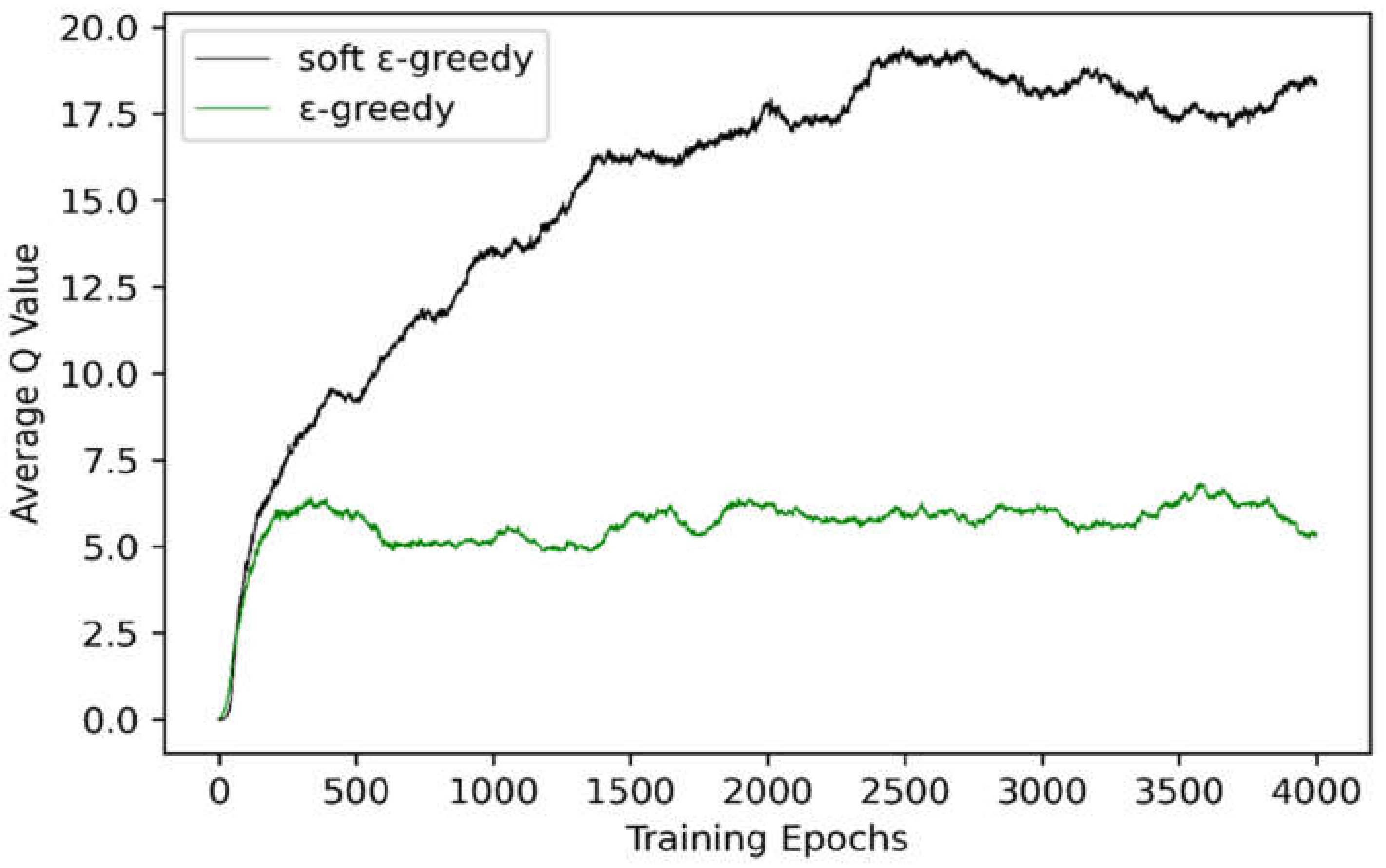
To demonstrate that the soft $\epsilon$-greedy behavior policy can reasonably balance exploration and exploitation depending on the problem size, the DDQN was trained for an instance with 10 machines, 50 new job arrivals and E_ave set to 50. For the soft $\epsilon$-greedy and $\epsilon$-greedy behavior policy, $\epsilon$ anneals linearly from 1 to 0.1. The linear annealing rate of $\epsilon$ is $\frac{1}{{\left(OP\_num\right)}^{1.8}}$ for the soft $\epsilon$-greedy policy, whereas the value is 0.001 for the $\epsilon$-greedy policy. During training, the parameter µ was set to 1.8; the values of the other hyperparameters are listed in Table 3. Through a method from the DQN literature [23], a fixed set of states was collected by running a random policy before the training started and the average of the maximum predicted $Q$ for these states was tracked. In Figure 4, the average predicted $Q$ of the soft $\epsilon$-greedy behavior policy is significantly higher than that of the $\epsilon$-greedy policy, indicating that the linearly decreasing rate of $\epsilon$ was adjusted according to the problem size, thus achieving a better compromise between exploration and exploitation and maximizing the cumulative reward.

4.3. Comparison of DDQN with Other Methods

To verify the effectiveness and generalization of the proposed DDQN, the DFJSP was classified according to different parameter settings for E_ave, m and n_add. To simulate a real production environment, the number of operations, delivery factors and penalty coefficients were distributed randomly for each job, so 30 independent instances were generated for each type of DFJSP. The DDQN was compared with two other RL algorithms, DQN and SARSA; one of the most commonly used heuristics algorithms, FIFO; and a famous metaheuristic algorithm, GA. Moreover, the random action selection policy RA was designed to prove the learning ability of the agent. In each instance, the DDQN and the other algorithms were repeated independently 20 times. The mean values of the total earliness and tardiness penalty obtained by each method are shown in

Table 5. Average total earliness and tardiness penalties of the different algorithms for each type of test (the best results are highlighted in bold font).

Eave	m	nadd	DDQN	DQN	SARSA	FIFO	GA	RA
30	5	20	5.17 × 103	6.63 × 103	7.27 × 103	1.35 × 104	1.07 × 104	1.41 × 104
		30	1.38 × 104	1.93 × 104	2.02 × 104	3.10 × 104	1.29 × 104	2.18 × 104
		50	3.68 × 104	4.42 × 104	4.64 × 104	7.02 × 104	4.97 × 104	5.55 × 104
		100	1.62 × 105	1.61 × 105	1.98 × 105	2.57 × 105	3.15 × 105	2.18 × 105
	10	20	1.48 × 103	2.26 × 103	3.02 × 103	4.42 × 103	3.53 × 103	4.08 × 103
		30	3.43 × 103	4.20 × 103	5.06 × 103	7.14 × 103	6.98 × 103	8.24 × 103
		50	9.26 × 103	1.12 × 104	1.15 × 104	1.78 × 104	1.38 × 104	1.90 × 104
		100	4.57 × 104	4.95 × 104	8.22 × 104	7.81 × 104	6.60 × 104	8.74 × 104
	30	20	5.31 × 103	6.10 × 103	6.29 × 103	6.11 × 103	6.41 × 103	6.40 × 103
		30	8.18 × 103	1.08 × 104	1.13 × 104	1.09 × 104	8.07 × 103	1.14 × 104
		50	8.03 × 103	1.31 × 104	1.43 × 104	1.35 × 104	1.09 × 104	1.52 × 104
		100	1.63 × 104	1.90 × 104	2.08 × 104	2.12 × 104	2.21 × 104	2.17 × 104
50	5	20	1.06 × 104	1.38 × 104	9.78 × 103	2.04 × 104	1.66 × 104	1.81 × 104
		30	1.94 × 104	2.34 × 104	2.91 × 104	3.69 × 104	2.65 × 104	3.07 × 104
		50	5.50 × 104	5.00 × 104	7.02 × 104	8.33 × 104	6.92 × 104	8.00 × 104
		100	1.61 × 105	1.86 × 105	2.26 × 105	2.88 × 105	2.64 × 105	2.27 × 105
	10	20	1.67 × 103	2.38 × 103	3.96 × 103	4.76 × 103	3.99 × 103	4.46 × 103
		30	3.29 × 103	4.22 × 103	8.13 × 103	7.61 × 103	7.46 × 103	9.18 × 103
		50	1.40 × 104	1.35 × 104	2.25 × 104	2.33 × 104	1.79 × 104	2.47 × 104
		100	5.88 × 104	6.46 × 104	7.24 × 104	9.64 × 104	7.72 × 104	9.18 × 104
	30	20	7.42 × 103	9.82 × 103	1.03 × 104	7.30 × 103	1.05 × 104	1.04 × 104
		30	9.06 × 103	1.20 × 104	1.25 × 104	1.23 × 104	1.20 × 104	1.26 × 104
		50	1.27 × 104	1.52 × 104	1.63 × 104	1.66 × 104	1.64 × 104	1.67 × 104
		100	1.85 × 104	2.22 × 104	2.29 × 104	2.33 × 104	2.15 × 104	2.47 × 104
100	5	20	9.10 × 103	1.20 × 104	1.38 × 104	2.12 × 104	1.47 × 104	1.95 × 104
		30	2.21 × 104	2.09 × 104	2.59 × 104	3.35 × 104	2.60 × 104	2.94 × 104
		50	5.11 × 104	5.50 × 104	5.80 × 104	9.16 × 104	6.72 × 104	7.46 × 104
		100	1.88 × 105	2.14 × 105	2.17 × 105	3.61 × 105	2.64 × 105	2.77 × 105
	10	20	3.68 × 103	4.42 × 103	4.98 × 103	6.67 × 103	6.35 × 103	6.95 × 103
		30	4.14 × 103	5.28 × 103	8.79 × 103	9.40 × 103	6.53 × 103	1.05 × 104
		50	1.19 × 104	1.62 × 104	1.17 × 104	2.35 × 104	1.84 × 104	2.71 × 104
		100	6.03 × 104	6.58 × 104	6.74 × 104	9.72 × 104	7.55 × 104	9.50 × 104
	30	20	8.58 × 103	8.49 × 103	1.12 × 104	1.18 × 104	1.14 × 104	1.17 × 104
		30	1.10 × 104	1.40 × 104	1.43 × 104	1.47 × 104	1.50 × 104	1.44 × 104
		50	1.34 × 104	1.83 × 104	1.87 × 104	2.02 × 104	2.02 × 104	1.98 × 104
		100	2.24 × 104	2.66 × 104	2.71 × 104	2.91 × 104	2.84 × 104	3.07 × 104

and the best results are highlighted in bold font.

In this study, the only difference between the DQN and the DDQN was the target y_i. Moreover, during training, $\epsilon$ decreased linearly from 1 to 0.1 in the DQN, while $\epsilon$ decreased from 1 to 0.01 in the DDQN. During testing, $\epsilon$ was fixed at 0.001.

In SARSA, in order to discretize the production state space reasonably, the neural network with a self-organizing mapping layer (SOM) from [19] was used to divide the state features into nine discrete states. The SARSA agent had the same action set of dispatching rules used in this study at each discrete state. A $Q$ table was maintained that contained 9 × 6 $Q$-values for the state–action pairs and the SARSA agent was trained to learn the policies linearly.

In GA [30], the chromosomes of the FJSP were encoded in the form of operation sequence (OS) and machine assignment (MS). In order to improve the response speed of production events, every individual of the initial population was randomly generated. The selection operation adopted a combination of the roulette wheel and the elite retention strategy. In the crossover operation, a uniform crossover was applied for MS and a precedence preserving order-based crossover (POX) was used for OS. The MS of the mutation operator adopted a multi-round single point exchange mutation and the OS part adopted a neighborhood search mutation. The hyperparameter settings were the population size N = 100, the number of iterations I = 200, the crossover probability p_c = 0.8 and the mutation probability p_m = 0.01.

FIFO choses the next operation of the earliest arriving job from among the unfinished jobs and the selected operation was assigned to the machine with the smallest sum of available time and processing time among the suitable machines. The RA was used to randomly select a dispatching rule at each rescheduling point.

In order to show the solution quality of the DDQN designed in this study, the average earliness and tardiness penalties of all the algorithms compared for all test instances were calculated according to Table 5, as shown in Figure 5. As can be seen in Figure 5, the DDQN outperformed the competing methods. The performance in terms of solution quality was normalized with respect to the average penalty of RA (that is, 100%). Note that the normalized performance of other algorithms, expressed as a percentage, was calculated as 100% * (algorithm penalty—RA penalty)/RA penalty. The normalized performance of the other algorithms was 33.80% (DDQN), 25.75% (DQN), 16.60% (SARSA), 1.68% (GA) and −13.32% (FIFO). It can also be seen that reinforcement learning (DDQN, DQN and SARSA) outperformed the competing methods (GA, RA and FIFO) in almost all instances, whereas deep reinforcement learning (DDQN and DQN) obtained a better solution quality than standard reinforcement learning with linear function approximation (SARSA).

To verify the generalization ability of DRL, the winning rate was defined, which was calculated as the number of instances in which the method achieved the best result divided by the number of all instances. Figure 6 presents the winning rate of all the algorithms calculated according to Table 4. Of the 36 test instances, the DDQN had the best results in 28 kinds of instances and the winning rate was 72.22%. The DQN has the smallest penalty for five scheduling problems and the winning rate was 13.89%. Both SARSA and GA had the minimum target value for two instances and the winning rate was 5.56%. The target value of FIFO was the smallest for one scheduling problem, with a winning rate of 2.78%. The winning rate of the random action strategy was 0%. The DDQN proposed in this study had the highest winning rate and performed at a level that was superior to the compared algorithms in general. Compared with RA, the DDQN obtained a lower total penalty in all test instances, demonstrating its ability to master difficult control policies for solving the DFJSP, to determine the proper dispatching rule at each rescheduling point.

It can be seen that on the whole, the DDQN clearly outperformed the other five methods in terms of solution quality and generalization. It is competent for solving the DFJSP with random job arrival to minimize penalties for earliness and tardiness. Reinforcement learning solves the scheduling problem as a Markov decision-making process and determines the ongoing action according to the production state to optimize the scheduling objectives.

5. Discussion

In this study, the DDQN was developed for the dynamic flexible job shop scheduling problem with random job arrival, aiming at optimizing the penalties for earliness and tardiness. In contrast to previous work [15,16,17,18,19,20], our approach provides DRL for the DFJSP in handling ongoing and weak correlation production states. Moreover, the soft ε-greedy strategy is designed to balance exploration and exploitation according to the problem scale, which improves the self-learning speed of the scheduling agent.

Because of the weak correlation between state features, the suitable number of dispatching actions and the DDQN architecture, the scheduling agent can achieve stable learning and convergence through training. Therefore, the training curve shows that the average penalties for earliness and tardiness drops smoothly with increasing training epochs. The proposed DRL allows the scheduling agent to learn the action–value function efficiently, to learn the optimal scheduling rules from the different production states. These comparison experiments show the DDQN-based scheduling agent outperforms the five compared methods in terms of solution quality and generalization.

The real-time optimization and decision-making of the DFJSP makes rapid and scientific response to customer orders and production emergencies and realizes intelligent matching between dispersed resources such as manpower, materials and machines. It improves the on-time delivery rate and reduces inventory and costs of enterprises. The proposed DRL provides reliable and robust scheduling schemes and meets customized production requirements according to dynamic changes in the production process. Cost, inventory, procurement, sales and transportation plans are automatically generated, which drives various management modules of enterprises around production. Therefore, the factory has the capabilities of self-learning and self-adaptation to realize intelligent decision-making.

For future work, more dynamic events like rush order insertions, stochastic processing time and machine breakdowns are worthy of investigation. Other objectives, such as machine utilization rate, energy consumption and makespan, will be considered to validate the generality of the proposed DDQN over different objectives. Meanwhile, there is not a single dispatching rule that performs well for all production environments [20], so the number of actions should be increased for a more general agent. However, a general state value that is shared across many similar actions is learned in many control tasks with large action spaces [31] and, consequently, introducing the dueling architecture [31] can be useful to improve the performance of the DDQN. In addition, since the DDQN is based on experience replay, which limits the methods to off-policy learning algorithms, we will apply state-of-the-art on-policy RL algorithms, such as an asynchronous advantage actor-critic algorithm (A3C) [32,33] and proximal policy optimization for solving the DFJSP.

6. Conclusions

This study introduced deep reinforcement learning for solving the DFJSP with random job arrival, to achieve the production goal of minimizing the penalties for earliness and tardiness. On the basis of constructing a mathematical model, the DDQN architecture of the DFJSP was constructed and the state features, the actions, the reward and the soft ε-greedy behavior policy were designed accordingly. Our approach indicated that the proposed DRL gave state-of-the-art results in 28 out of 36 production instances, compared with DQN, SARSA, FIFO, GA and RA, without changing the architecture or hyperparameters of the deep network.