Article

Audio Compensation with Cascade Biquad Filters for Feedback Active Noise Control Headphones

School of Mechanical and Automotive Engineering, Qingdao University of Technology, Qingdao 266520, China
*
Authors to whom correspondence should be addressed.
Processes 2022, 10(4), 730; https://doi.org/10.3390/pr10040730
Submission received: 15 March 2022 / Revised: 8 April 2022 / Accepted: 8 April 2022 / Published: 9 April 2022
(This article belongs to the Special Issue Advanced Processes Creating New Technologies in Tomorrow's Industry)

Abstract

:
In active noise control (ANC) headphones, the audio signal is modified together with the primary noise if a feedback controller is used. Although this problem can be alleviated with an FIR model of the secondary path, practical implementations are usually restricted by its computational complexity. In this paper, cascade biquad filters are used to compensate for the modification of the audio system. Instead of using classical identification methods with an IIR model, the audio compensation problem is fixed through an optimization process. An objective function evaluating the comprehensive compensation performance is proposed, whose minimum value is obtained using the differential evolution (DE) algorithm. Simulations and experiments are carried out, whose results validate the effectiveness and efficiency of the proposed optimization method. The averaged compensation error can be reduced to about 0.5 dB with only two to five biquad filters.

1. Introduction

The environmental noise can greatly degrade the listening quality when enjoying music with headphones. Compared with increasing the music level to mask the annoying noise, designing noise-proof headphones generally offers a better way to overcome this problem. Although passive strategies are efficient to block noise at relatively high frequencies, residual low-frequency noise remains a problem with limited volumes and weights in real applications. Active noise control (ANC) [1,2] offers a solution to deal with such low-frequency residual noises, whose application in headphones has been investigated for decades. Both feedforward [3,4,5] and feedback [6,7,8] controllers can be considered to design an ANC headphone, whose effectiveness was confirmed. Compared with traditional adaptive algorithms, fixed controllers designed with cascade biquad filters [5,7,8] have much lower computational complexities. This generally indicates a lowered cost together with a lengthened battery life, which is crucial for commercial products. Meanwhile, the sampling frequency can also be enhanced, leading to a lowered latency with which the limitation on the control performance could be alleviated. To the best of the authors’ knowledge, in recent years various commercial chips specially designed for headphones have integrated cascade biquad or IIR filters as the internal ANC controllers, which could lead to wide applications for ANC headphones.
Compared with a feedforward ANC controller [3,4,5], more attention should be paid to the audio system when using a feedback controller [6,7,8]. Since the error microphone can pick up the audio signal played by the speaker, the low-frequency components of the audio signal will also be attenuated together with the environmental noise [1]. This problem can be overcome by the usage of an FIR model of the secondary path [9,10], with which the audio signal component picked up by the error microphone can be estimated and then subtracted from the error signal. With a secondary path model without modeling errors, the audio signal component of the error signal would be totally neutralized and thus the audio system would not be affected by the ANC system. An online secondary path identification scheme can further be considered in which the audio signal is used as a natural stimulus. This method can be extended to other ANC areas with feedback controllers, such as infant incubators [11], hearing aids [12], or even road noise control in vehicles [13]. Moreover, it was reported that virtual bass enhancement could also be considered as another technique to enhance the audio quality of the ANC headphones [14].
Although the audio compensation method with an FIR model of the secondary path was proven to be effective, it cannot be directly used in commercial ANC headphone chips where only biquad or IIR filters are available. Perkmann and Tiefenthaler [15] proposed a similar scheme for audio compensation. In their patent, the FIR model is replaced with one or more lowpass filters, which can be realized with cascade biquad or IIR filters. However, no audio compensation results were given. Generally speaking, there is still a lack of audio compensation methods for feedback ANC headphones with the usage of cascade biquad filters, which is indispensable for commercial products. This is the main motivation for this work.
In this paper, an optimization process is proposed for the audio compensation of feedback ANC headphones, where the compensation filter is constructed with cascade biquad filters. Instead of identifying the secondary path with an IIR model, an objective function corresponding to the audio compensation performance is established, with which the optimal cascade biquad filters are searched. In the proposed optimization process, the biquad filter is parameterized into three prototypes, and both the prototypes and the corresponding parameters are automatically optimized. The differential evolution (DE) [16,17] algorithm is used to find the optimal solution, whose efficiency was confirmed by the optimization of feedforward ANC controllers [5], as well as the feedback ones [8]. Compared with the methods presented in [5,7,8], where only two prototypes of biquad filters are used and the combinations of filter prototypes are just set by experiences, the proposed method could address more flexibility in the optimization process. In Section 2, both a classical IIR identification method and the proposed method are described in detail. Simulations and experiments are further carried out in Section 3, whose results show that the proposed method is more efficient than the existing methods.

2. Methods

2.1. Identification of the Secondary Path with an IIR Model

Although the environmental noise can be efficiently attenuated by the feedback controller of an ANC headphone, the low-frequency components of the input audio signal would also be reduced at the same time. Figure 1a gives a solution to this problem, where a compensation filter H(z) is used and its output is subtracted from the error signal picked up by the error microphone. Generally, a model of the secondary path S(z) is used for H(z) [9,10,11,12,13], in which case the audio component of the error signal would be totally eliminated if the model is accurate enough. Since the input of the feedback controller C(z) is no longer related to the audio signal, the audio system of the headphone would not be altered when the ANC system is turned on. This can be directly observed from the following equation:
G e q ( z ) = Y ( z ) X ( z ) = 1 C ( z ) H ( z ) 1 C ( z ) S ( z )
where the transfer function between the audio input signal X(z) and the secondary path’s input signal Y(z) is defined.
Although FIR models of the secondary path are widely used in the literature on ANC, their realization for headphones might be a problem with ANC chips where only biquad or IIR filters are available. As a result, in such cases, an IIR model filter H(z) should be used instead
H ( z ) = i = 0 M b i z i 1 i = 1 M a i z i = B ( z ) 1 A ( z )
where bi (i = 0, 1, …, M), ai (i = 1, 2, …, M) are the coefficients of the numerator polynomial B(z) and the denominator polynomial A(z), respectively, and M is the filter order. In order to obtain accurate estimations of these coefficients, a classical IIR identification method [2] is illustrated in Figure 1b, where v(n) is the stimulus and d(n) is the tested output of the target system. In the identification process, the output of the model filter is calculated with the following equation:
u ( n ) = i = 0 M b i v ( n i ) + i = 1 M a i d ( n i )
and a so-called equation error is used to adjust the coefficients of B(z) and A(z)
e ( n ) = d ( n ) u ( n )
Since the input of the tapped delay line of A(z) is the exact desire signal d(n), only errors in the coefficients are responsible for the mean square value of e(n). Meanwhile, as the output of the IIR model is the sum of two independent FIR filter outputs, the equation error is a linear function with respect to the coefficients. Thus, the mean square error is a quadratic function with a single minimum. Although the LMS algorithm can be used here, its convergence rate might be reduced since d(n) is not white. Considering that the LMS algorithm would finally converge to the Wiener solution, the optimal coefficients could be directly calculated using the Wiener–Hopf equation so that the relatively long convergence of the LMS algorithm could be avoided.
With the definition of a combined input vector r(n) and the coefficient vector c
r ( n ) = [ v ( n ) , , v ( n M ) , d ( n 1 ) , , d ( n M ) ] T c = [ b 0 , , b M , a 1 , , a M ] T
the Wiener–Hopf equation can be expressed as
E [ r ( n ) r T ( n ) ] c = E [ r ( n ) d ( n ) ]
where E[·] denotes the mathematical expectation.
Instead of using the LMS algorithm, the auto-correlation function of r(n), as well as the cross-correlation function between r(n) and d(n), are estimated first in this work. The coefficients ai, bi are then calculated using the Wiener–Hopf equation shown by (6). The identified M-order IIR model can finally be converted into a series of cascade biquad filters for real applications.

2.2. Compensation with Optimized Cascade Biquad Filters

Instead of identifying the secondary path with an IIR model, an optimization procedure for the compensation filter H(z) is proposed with cascade biquad filters in this paper. Three prototypes of the biquad filter [18] are used here, whose transfer functions are shown as follows:
H 0 ( z ) = ( 1 + α A ) 2 c o s ω z 1 + ( 1 α A ) z 2 ( 1 + α / A ) 2 c o s ω z 1 + ( 1 α / A ) z 2
H 1 ( z ) = A ( ( A + 1 ) + ( A 1 ) c o s ω + 2 α A ) 2 ( ( A 1 ) + ( A + 1 ) c o s ω ) z 1 + ( ( A + 1 ) + ( A 1 ) c o s ω 2 α A ) z 2 ( ( A + 1 ) ( A 1 ) c o s ω + 2 α A ) + 2 ( ( A 1 ) ( A + 1 ) c o s ω ) z 1 + ( ( A + 1 ) ( A 1 ) c o s ω 2 α A ) z 2
H 2 ( z ) = 1 2 ( 1 c o s ω ) ( 1 + 2 z 1 + z 2 ) ( 1 + α ) 2 c o s ω z 1 + ( 1 α ) z 2
The parameters in (7)–(9) are defined as follows with a sampling frequency fs:
A = 1 0 g 40 , ω = 2 π f f s , α = s i n ω 2 Q
With the definitions in (10), the magnitude response for H0(z) is enhanced by g dB at f Hz, while the one for H1(z) is enhanced by g dB below f Hz. Thus, H0(z) and H1(z) can be regarded as the peak/notch and low/high shelf filters with g > 0 or g < 0, respectively. It can be observed that H0(z) and H1(z) are both minimum phase filters and are identical to the ones used in the controller design for feedforward [5] and feedback [8] ANC headphones. Since the secondary path is not a minimum phase system, apparently only using the first two prototypes might not be enough for the audio compensation. Thus, a third prototype is added to this paper. In (7), H2(z) is a non-minimum phase lowpass filter with a cutoff frequency of f Hz. It can be found that the parameter A and g is absent for this lowpass filter. For all three prototypes, Q is the quality factor. The frequency responses around f Hz vary with different values of Q.
The compensation filter H(z) is cascaded with N prototype filters
H ( z ) = 1 0 G a i n / 20 i = 1 N H i ( z )
where Gain is an extra gain for H(z). Consequently, the transfer function of H(z) is determined by the following parameter vector:
θ = [ t p 1 , g 1 , f 1 , Q 1 , , t p N , g N , f N , Q N , G a i n ]
where gi, fi, Qi are the parameters defined in (10) corresponding to the i-th biquad filter Hi(z).
Different from the methodologies when designing ANC controllers [5,8], the prototype of the i-th filter Hi(z) is also defined as a parameter tpi in this paper
H i ( z ) = { H 0 ( z ) 0 t p i < 1 H 1 ( z ) 1 t p i < 2 H 2 ( z ) 2 t p i < 3
with which the frequency response of H(z) could be more flexible.
In order to optimize the compensation filter H(z), an objective function is proposed as follows:
O b j = 20 k w k l g | G e q ( e j 2 π f k / f s ) | + ξ [ s u m ( U ( l b θ ) ) + s u m ( U ( θ u b ) ) ]
In the first term on the right-hand side of (14), the absolute value of Geq(z) with dB as its unit is used to evaluate the performance of the audio compensation, which indicates that the compensated audio signal should have the same amplitude as the original one. A weighted sum of this value over different frequencies fk is used to evaluate the performance within the whole frequency band (20, 20 k) Hz for audio systems, where wk is the weighting coefficient corresponding to fk. From (1) it could be seen that, in order to calculate Geq(z), the frequency responses of the secondary path S(z) and the feedback controller C(z) should be known as a priori, which indicates H(z) should be optimized after S(z) is tested and C(z) is designed.
The second term on the right-hand side of (14) is a punishment term where U(x) is the unit step function
U ( x ) = { 1 x 0 0 x < 0
and sum(x) denotes the summation over the vector x. This term represents the constraint on the bounds of the parameter vector θ, and lb, ub are the pre-defined lower and upper bounds of θ, respectively. By choosing a proper punishment intensity ξ, a large value would be injected into the objective function if one or more parameters in θ exceed the pre-defined bounds. As a result, θ would be restricted within [lb, ub] when trying to minimize Obj.
With definitions of (7)–(15), an optimization problem can be proposed as:
θ = m i n { O b j | θ }
which tries to find the optimum audio compensation performance directly and is rather different from acquiring an accurate IIR model.
Since the objective function is rather complex with respect to θ, the DE algorithm [16,17] is used to solve the proposed optimization problem, which is arguably one of the most powerful stochastic real-parameter optimizers in current use [16]. The DE algorithm has the advantages of simple and straightforward implementations, low space complexity, as well as competitive optimization ability compared with other optimizers [17]. Although some strong algorithms were able to beat DE in some competitions, the simple implementation, as well as the overall performance of DE (in terms of accuracy, convergence speed, and robustness), still make it attractive for solving the optimization problem described in this paper. The efficiency of the DE algorithm has already been confirmed through the controller optimizations for both feedforward [5] and feedback [8] ANC headphones. There are only three controlling parameters within the DE algorithm, which are the crossover rate Cr, the stepsize F and the population members NP, respectively. It is recommended that the optimization process with DE should be repeated multiple times since the algorithm could still be trapped in local minimums. It is further noted that other algorithms could also be considered to solve the proposed optimization problem, such as Quantum-behaved Particle Swarm Optimization (QPSO) [19] or Grey Wolf Optimizer (GWO) [20]. A detailed comparison for different optimizers can be found in [20], which shows that the DE algorithm could still be considered to be quite competitive.

3. Results

In this section, experiments are carried out to evaluate the presented methods. 
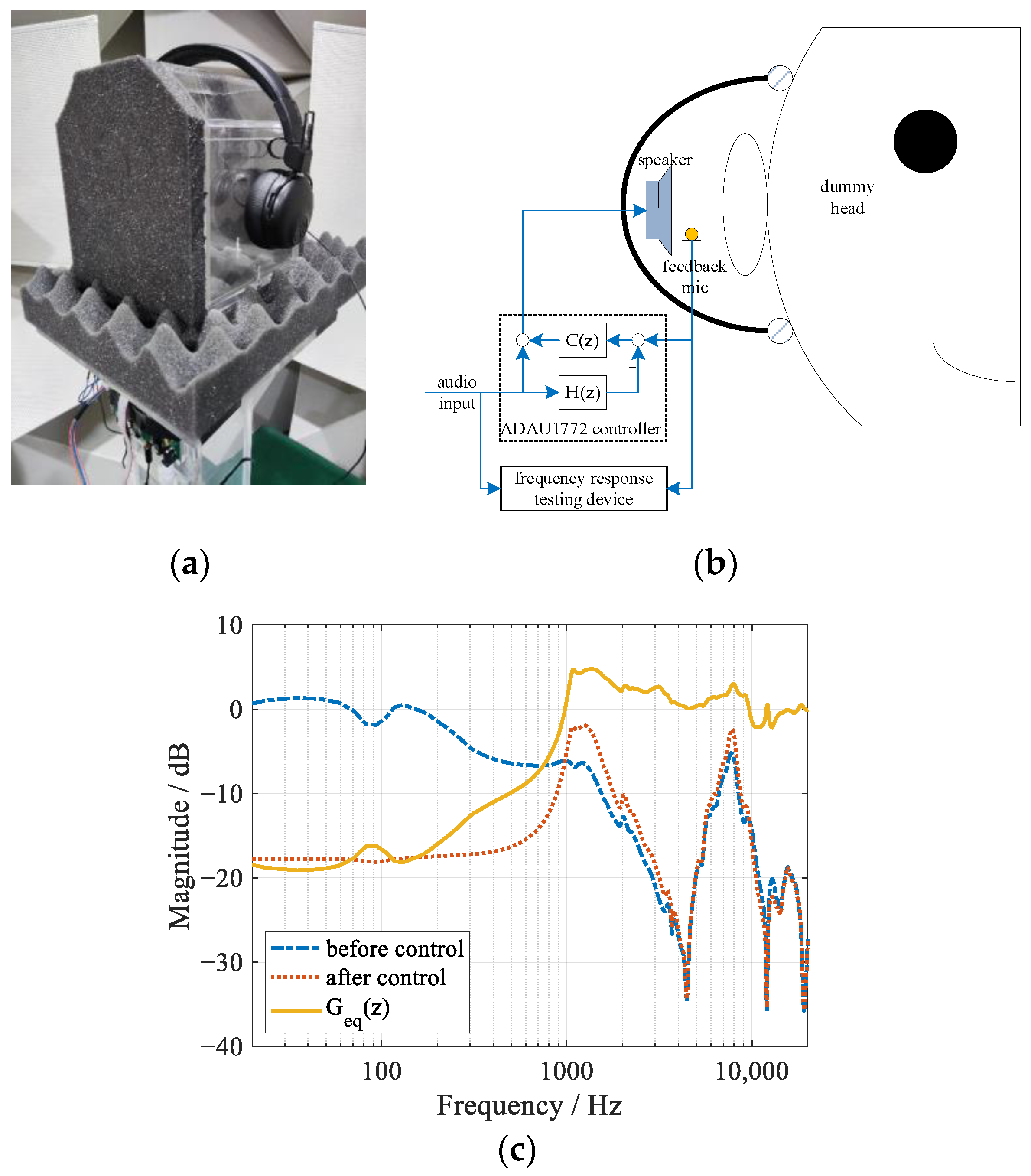
Figure 2a,b show the experimental setup, where a self-designed dummy head is used together with a commercial feedback ANC headphone. The feedback microphone and the speaker of the ANC headphone are wired to an outside controller with an ADAU1772 chip as its processor, as shown in Figure 2b. Both the feedback controller C(z) and the compensation filter H(z) are implemented inside this processor, within which the sampling frequency is set to 192 kHz. For the feedback controller, a previous design result in [8] is used here, with which the primary noise could be effectively attenuated. However, the response of the audio system, which is the system between the audio input signal and the output signal of the feedback microphone, will also be altered by this feedback controller. In the experimental system, an external device is used to test the frequency response of the audio system with white noise as the stimulus, as shown in Figure 2b. Figure 2c compares the magnitude responses of the audio system before and after the feedback controller is turned on. It can be seen that, without audio compensation (H(z) = 0), the low-frequency components of the audio signal are attenuated just as the primary noise, while some high-frequency components would be enhanced because of the waterbed effect [1]. The difference between these two responses is given as the yellow line in Figure 2c at the same time, which is also the magnitude response of Geq(z) without audio compensation. Meanwhile, it is further noted that this curve is theoretically identical to the noise reduction performance of the feedback controller with respect to the primary noise.
In order to get rid of the influence caused by the feedback controller, the conventional method with an FIR model of the secondary path is first evaluated. Using the recorded input (white noise) and output of the secondary path, a full-length FIR model (filter order M = 1000) is obtained with the LMS algorithm, whose result is shown in Figure 3a. Since the computational complexity is rather high, different truncations of this FIR model (i.e., just taking the first M coefficients of the full-length model) are used for the audio compensation, whose results are illustrated in Figure 3b–e. Figure 3b,c compare the magnitude and phase responses of the truncated FIR models with the original responses of the secondary path. It can be seen that the modeling accuracy increases as M becomes higher. The modeling errors mainly appear within the low-frequency band, which results from the relatively low-frequency resolution of the truncated FIR models. With these truncated FIR models, the audio compensation performance is further shown in Figure 3d, where the magnitude responses of the audio system are illustrated. This compensated response should be close to the original secondary path S(z) as much as possible so that the audio system would not be affected by the feedback control system. In fact, the compensated audio response would be identical to the original S(z) if an accurate model is used as the compensation filter. However, there would still be some compensation errors because of the inevitable modeling errors. It can be seen that, although the audio system is less affected by the feedback control system compared with Figure 2c, the audio responses still mismatch with the original one at low frequencies, which is a natural result of the relatively large modeling errors within this frequency range. Figure 3e shows the magnitude response of Geq(z), which can be regarded as compensation errors. It can be observed that large compensation errors mainly appear at low frequencies, which would decrease as the filter order M becomes higher. A good compensation performance can be obtained when M reaches 400.
Next, the secondary path is identified with IIR models using the method presented in Section 2.1. In order to enhance the modeling accuracy within the low-frequency band where the degradation of the audio system is significant, pink noise is used as the stimulus for the identification process. With the recorded input and output signals of the secondary path, the auto-correlation and cross-correlation functions are estimated first. Then, IIR models with different orders M can be obtained by solving the Wiener–Hopf equation shown in (6). It is noted that this M-order IIR model could be realized by N = M/2 cascade biquad filters in applications. Figure 4a,b show the magnitude and phase responses of the obtained IIR models, respectively, which are compared with the original response of the secondary path S(z). It can be found that the modeling accuracy increases when the filter order becomes higher. With these IIR models, the compensation performance for the audio system can be calculated, whose results are shown in Figure 4c,d. Figure 4c gives the compensated magnitude responses of the audio system with feedback control. Compared with Figure 3c, it can be observed that the compensation performance at low frequencies is enhanced but relatively large mismatches still appear around 1 kHz. Figure 4d illustrates the corresponding compensation errors. It can be observed that the compensation errors could be restricted within ±3.5 dB with a 4th-order IIR model. With more accurate models, however, the compensation errors show greater peak values at about 1 kHz. This indicates that the modeling errors have different influences on the compensation performance at different frequencies, which is not considered in the identification process. When the IIR filter order becomes relatively large, the compensation errors can be reduced to a low level, since an IIR model with enough accuracy could be obtained in this case.
The averaged absolute values of the compensation errors are further calculated for both FIR and IIR models, whose results are shown in Figure 5. It can be observed from Figure 5a that generally, the averaged error decreases as the order increases for both cases. For the truncated FIR models, a good performance could be expected with M greater than 300. For the IIR models, in order for a good compensation performance, more than 30 biquad filters (M > 60) should be used.
The compensation performance is further compared with respect to the computational complexity in Figure 5b. The required number of multiplications is evaluated here since it is generally more time-consuming than additions. For an M-order FIR filter, M multiplications are needed. For an M-order IIR filter, which is realized with N = M/2 cascade biquad filters, the number of multiplications is 2.5 M since each biquad filter needs five multiplications. It can be observed from Figure 5b that, with similar performance, the computational complexity is larger if truncated FIR models are used. Although the computational complexity is relatively low for IIR models, the required number of biquad filters still seems too large to be realized by a low-cost ANC processor such as ADAU1772, considering that an effective feedback controller can be constructed with only three to five biquad filters [7,8].
In order for a good compensation performance with fewer biquad filters, the optimization problem proposed in Section 2.2 is solved using the DE algorithm with respect to different numbers of biquad filters. In the objective function, Geq(z) is evaluated at 300 discrete frequencies fk, which are chosen logarithmically from 20 Hz to 20 kHz. All the weighting coefficients wk are set to 1, which addresses the same significance to the compensation performance over the whole audio frequency band. The searching intervals for tpi, gi, fi, Qi and Gain are bounded within [0, 3], [−40, 40] dB, [20, 20k] Hz, [0.1, 3.0] and [−40, 40] dB, respectively. The punishment intensity ξ is set to 10,000. In the DE algorithm, Cr, F, and NP are set to 1, 0.85, and 100, respectively. For each case of N, 100 times repeat of the DE algorithm is conducted to avoid local minimums. In every single run, the DE algorithm stops searching after 20,000 iterations. For each case of N, the learning curve of the DE algorithm corresponding to the optimal solution is shown in Figure 6. It can be seen that the DE algorithm would converge to a lower value of the objective function if N becomes higher. Although the algorithm does not appear to be fully converged for the case of N = 6, a better solution could still be found. The obtained results are listed in Table 1. It can be found that lowpass filters seem to be necessary for each case of N, while peak/notch or shelf filters are optional. The reason might lie in the non-minimum phase response of H2(z), which is similar to the secondary path. It can also be seen that the combinations of filter types are different from case to case. It is for this reason that the filter types are designed to be variables in the proposed optimization method. Moreover, this optimization strategy with variable filter types could also be considered for the design of feedforward [5] and feedback [8] controllers.
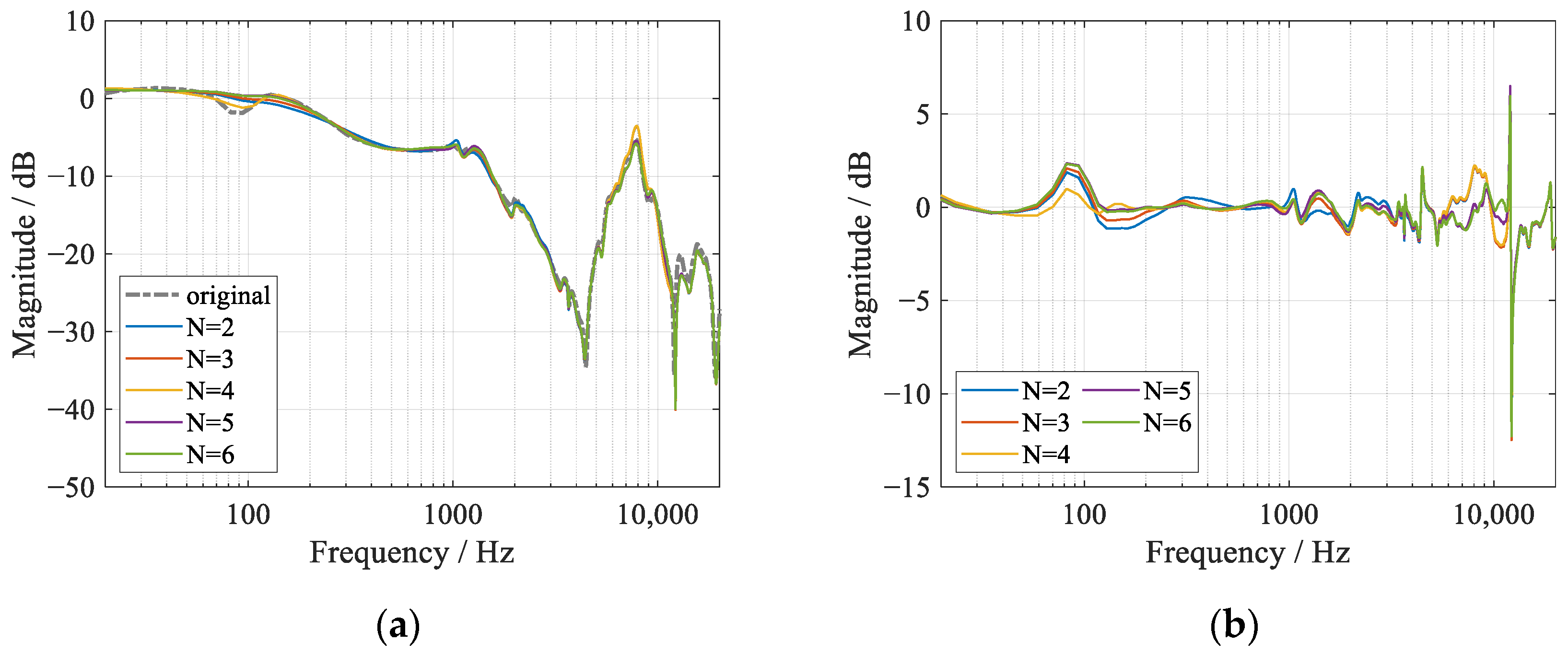
Figure 7a,b show the magnitude and phase responses of the compensation filter H(z) with N = 2, 3, 4, 5, 6, and Figure 7c,d show the compensated audio responses, as well as the corresponding compensation errors. It can be observed that the compensation filter still tries to model the secondary path, especially within the frequency band below about 3 kHz. Within this frequency range, the control performance of the feedback controller could be considered to be obvious. Compared with Figure 4, it can be observed that the modeling accuracy here is much higher within this frequency range, which results in better compensation performances, as shown in Figure 7c,d. With fewer biquad filters (N = 2, 3, 4), H(z) is essentially a low-pass filter and the audio components are attenuated above 3 kHz. If N increases to 5 and 6, however, H(z) has extra abilities to model the peak response within (5, 10) kHz of the secondary path. As a result, a better compensation performance within this frequency range could be obtained. It can be seen from Figure 7c that, with the optimized compensation biquad filters, the audio responses with feedback control are in high accordance with the original secondary path S(z), which indicates the influence of the feedback controller on the audio system was successfully depressed.
Similar to the case with FIR and IIR models, the averaged compensation errors are calculated and compared in Figure 5. It can be found that with the same number of biquad filters, the proposed optimization method behaves much better than using an identified IIR model. Meanwhile, an averaged error of about 0.5 dB can be obtained with only two to five biquad filters. The corresponding computational complexity is the lowest compared with the other two methods if a similar performance is assumed to be achieved, which is beneficial for real applications. Although using more biquad filters can lead to better performance, the DE algorithm might have more difficulties in finding the global minimum when N is greater than 6, as indicated in Figure 6. On the other hand, by comparing the performance with the 1000-order FIR model in Figure 5, it can be expected that, when N > 6, the performance would not be enhanced obviously even if the global optimum solutions were found. Consequently, two to five biquad filters are suggested based on the results obtained in this paper, which are proven to be adequate to achieve good performance for the audio compensation.
Finally, the coefficients of the designed compensation filters are downloaded into ADAU1772, and the responses of the audio system after compensation are tested as illustrated in Figure 2b, whose results are shown in Figure 8a. Figure 8b shows the corresponding compensation errors with respect to the original response of the secondary path. It can be found that the experiment results match the simulation results very well, although relatively large errors appear at about 12 kHz, which mainly result from the drift of the corresponding notch frequency of the secondary path response.

4. Conclusions

For ANC headphones, the response of the audio system will be modified by the feedback controller, which could generally be resolved by the usage of an FIR model of the secondary path. Compared with FIR filters, cascade biquad filters have the advantage of low computational complexity and can greatly ease practical implementations. However, how to compensate for the modified audio system with such IIR filters remains a problem. Although the classical identification method with an IIR model of the secondary path can be considered, it was found that a relatively high number of biquad filters are needed to provide a model with enough accuracy so that a good compensation performance of the audio system can be expected.
Instead of identifying the secondary path, an optimization process is proposed for the compensation filter in this paper. The biquad filters are parameterized into three prototypes and an objective function is developed to evaluate the comprehensive compensation performance. An optimization problem is then proposed and the DE algorithm is used to find its optimal solution. Both the filter prototypes and their parameters are automatically optimized in the proposed method. Simulations and experiments are carried out to validate the proposed method. The results have shown that the designed compensation filter also tries to model the secondary path but with higher accuracy in the frequency range where the response of the audio system is biased more obviously. With the proposed optimization process, a good compensation performance can be obtained with only two to five biquad filters, in which case the averaged compensation error can be reduced to about 0.5 dB.

Author Contributions

Conceptualization, F.A.; methodology, F.A.; software, F.A.; validation, F.A.; formal analysis, F.A.; investigation, F.A.; data curation, Q.W.; writing—original draft preparation, F.A.; writing—review and editing, Q.W. and B.L.; supervision, B.L.; project administration, B.L.; funding acquisition, B.L. All authors have read and agreed to the published version of the manuscript.

Funding

This research is funded by the National Natural Science Foundation of China (grant number 11404367, 51905288, 11874034), the Taishan Scholar Program of Shandong (No. ts201712054) and the Shandong Science and Technology Enterprise Innovation Capacity Enhancement Project (2021TSGC1036).

Institutional Review Board Statement

Not applicable.

Informed Consent Statement

Not applicable.

Data Availability Statement

The data presented in this study are available on request from the corresponding author.

Conflicts of Interest

The authors declare no conflict of interest.

References

  1. Elliott, S.J. Signal Processing for Active Control; Academic Press: London, UK, 2001. [Google Scholar]
  2. Hansen, C.; Snyder, S.; Qiu, X.; Brooks, L.; Moreau, D. Active Control of Noise and Vibration; CRC Press: Boca Raton, FL, USA, 2012. [Google Scholar]
  3. Patel, V.; Cheer, J.; Fontana, S. Design and implementation of an active noise control headphone with directional hear-through capability. IEEE Trans. Consum. Electron. 2020, 66, 32–40. [Google Scholar] [CrossRef]
  4. Belyi, V.; Gan, W.S. A combined bilateral and binaural active noise control algorithm for closed-back headphones. Appl. Acoust. 2020, 160, 107129. [Google Scholar] [CrossRef]
  5. An, F.; Liu, B. Cascade biquad controller design for feedforward active noise control headphones considering incident noise from multiple directions. Appl. Acoust. 2022, 185, 108430. [Google Scholar] [CrossRef]
  6. Kuo, S.M.; Chen, Y.R.; Chang, C.Y.; Lai, C.W. Development and Evaluation of Light-Weight Active Noise Cancellation Earphones. Appl. Sci. 2018, 8, 1178. [Google Scholar] [CrossRef] [Green Version]
  7. Wang, J.; Zhang, J.; Xu, J.; Zheng, C.; Li, X. An optimization framework for designing robust cascade biquad feedback controllers on active noise cancellation headphones. Appl. Acoust. 2021, 179, 108081. [Google Scholar] [CrossRef]
  8. An, F.; Wu, Q.; Liu, B. Feedback Controller Optimization for Active Noise Control Headphones Considering Frequency Response Mismatch between Microphone and Human Ear. Appl. Sci. 2022, 12, 977. [Google Scholar] [CrossRef]
  9. Gan, W.S.; Kuo, S.M. An integrated audio and active noise control headset. IEEE Trans. Consum. Electron. 2002, 48, 242–247. [Google Scholar] [CrossRef]
  10. Chang, C.Y.; Siswanto, A.; Ho, C.Y.; Yeh, T.K.; Chen, Y.R.; Kuo, S.M. Listening in a noisy environment: Integration of active noise control in audio products. IEEE Trans. Consum. Electron. Mag. 2016, 5, 34–43. [Google Scholar] [CrossRef]
  11. Kuo, S.M.; Liu, L.; Gujjula, S. Development and application of audio-integrated ANC system for infant incubators. Noise Control Eng. J. 2010, 58, 163–175. [Google Scholar] [CrossRef]
  12. Ho, C.Y.; Shyu, K.K.; Chang, C.Y.; Kuo, S.M. Integrated active noise control for open-fit hearing aids with customized filter. Appl. Acoust. 2018, 137, 1–8. [Google Scholar] [CrossRef]
  13. Sano, H.; Inoue, T.; Takahashi, A.; Terai, K.; Nakamura, Y. Active control system for low-frequency road noise combined with an audio system. IEEE Trans. Speech Audio 2001, 9, 755–763. [Google Scholar] [CrossRef]
  14. Coker, K.; Shi, C. A Survey on Virtual Bass Enhancement for Active Noise Cancelling Headphones. In Proceedings of the IEEE International Conference on Control, Automation and Information Sciences (ICCAIS), Chengdu, China, 23–26 October 2019. [Google Scholar] [CrossRef]
  15. Perkmann, M.; Tiefenthaler, P. Noise Reducing Sound Reproduction System. U.S. Patent 9,613,612, 4 April 2017. [Google Scholar]
  16. Das, S.; Suganthan, P.N. Differential evolution: A survey of the state-of-the-art. IEEE Trans. Evolut. Comput. 2011, 15, 4–31. [Google Scholar] [CrossRef]
  17. Ahmad, M.F.; Isa, N.A.M.; Lim, W.H.; Ang, K.M. Differential evolution: A recent review based on state-of-the-art works. Alex. Eng. J. 2022, 61, 3831–3872. [Google Scholar] [CrossRef]
  18. Bristow-Johnson, R.; Schepers, D. Cookbook Formulae for Audio Equalizer Biquad Filter Coefficients. Cookbook Formulae for Audio EQ Biquad Filter Coefficients. Available online: www.w3.org/2011/audio/audio-eq-cookbook.html (accessed on 3 April 2022).
  19. Omkar, S.N.; Khandelwal, R.; Ananth, T.V.S.; Naik, G.N.; Gopalakrishnan, S. Quantum behaved Particle Swarm Optimization (QPSO) for multi-objective design optimization of composite structures. Expert Syst. Appl. 2009, 36, 11312–11322. [Google Scholar] [CrossRef]
  20. Mirjalili, S.; Mirjalili, S.M.; Lewis, A. Grey wolf optimizer. Adv. Eng. Softw. 2014, 69, 46–61. [Google Scholar] [CrossRef] [Green Version]
Figure 1. The schematic diagrams of (a) the feedback ANC headphone with audio compensation and (b) the system identification method with an IIR model using the equation error.
Processes 10 00730 g001
Figure 2. The experimental feedback ANC headphone: (a) the photo, and (b) the schematic diagram of the system, (c) the variation of the magnitude response of the audio system before and after feedback control without audio compensation.
Processes 10 00730 g002
Figure 3. Simulation results with truncated FIR models of the secondary path for audio compensation: (a) the full-length FIR model of the secondary path, the (b) magnitude and (c) phase responses of the truncated FIR models with different orders, (d) the magnitude responses of the compensated audio system and (e) the compensation errors.
Processes 10 00730 g003aProcesses 10 00730 g003b
Figure 4. Simulation results with identified IIR models of the secondary path for audio compensation: the (a) magnitude and (b) phase responses of the IIR models with different orders, (c) the magnitude responses of the compensated audio system and (d) the compensation errors.
Processes 10 00730 g004aProcesses 10 00730 g004b
Figure 5. Averaged compensation errors using different methods with respect to (a) the filter order and (b) the computational complexity.
Processes 10 00730 g005
Figure 6. Learning curves of DE algorithm corresponding to the optimal solutions.
Processes 10 00730 g006
Figure 7. Simulation results using optimized compensation filter H(z): the (a) magnitude and (b) phase responses of H(z) with different numbers of cascade biquad filters, (c) the magnitude responses of the compensated audio system and (d) the compensation errors.
Processes 10 00730 g007
Figure 8. Experiment results using optimized compensation filter H(z): (a) the magnitude responses of the compensated audio system and (b) the compensation errors.
Processes 10 00730 g008
Table 1. Design results for the parameter vector of the compensation filter H(z).
Biquad FilterParametersN = 2N = 3N = 4N = 5N = 6
Filter 1Filter typelowpassshelfnotchlowpassshelf
g (dB)-18.3−32.3-9.5
f (Hz)908.25.00 k8.79 k1.37 k267.2
Q0.180.100.100.960.68
Filter 2Filter typepeaknotchlowpasslowpasspeak
g (dB)9.9−3.8--31.99
f (Hz)1.27 k444.01.63 k10.26 k11.32 k
Q0.810.670.543.001.12
Filter 3Filter type-lowpassshelfshelfnotch
g (dB)-−14.78.5−13.5
f (Hz)1.34 k786.8255.43.96 k
Q0.990.720.712.19
Filter 4Filter type--shelflowpasslowpass
g (dB)−1.5--
f (Hz)116.27.72 k1.21 k
Q2.133.001.01
Filter 5Filter type---shelflowpass
g (dB)−8.1-
f (Hz)5.41 k7.71 k
Q3.003.00
Filter 6Filter type----shelf
g (dB)26.1
f (Hz)15.93 k
Q2.97
Gain (dB)1.3−17.117.60.6−34.5
Publisher’s Note: MDPI stays neutral with regard to jurisdictional claims in published maps and institutional affiliations.

