Object Detection Algorithm for Surface Defects Based on a Novel YOLOv3 Model

Abstract

The surface defects of industrial structural parts have the characteristics of a large-scale span and many small objects, so a novel YOLOv3 model, the YOLOv3-ALL algorithm, is proposed in this paper to solve the problem of precise defect detection. The K-means++ algorithm is combined with the intersection-over-union (IoU) and comparison of the prior box for clustering, which improves the clustering effect. The convolutional block attention module (CBAM) is embedded in the network, thus improving the ability of the network to obtain key information in the image. By adding fourth-scale prediction, the detection capability of a YOLOv3 network for small-object defects is greatly improved. A loss function is designed, which adds the generalized intersection-over-union (GIoU) loss combined with focal loss to solve the problems of L2 loss and class imbalance in samples. Experiments regarding contour-defect detection for stamping parts show that the mean average precision (mAP) of the YOLOV3-ALL algorithm reaches 75.05% in defect detection, which is 25.16% higher than that of the YOLOv3 algorithm. The average detection time is 39 ms/sheet. This proves that the YOLOv3-ALL algorithm has good real-time detection efficiency and high detection accuracy.

1. Introduction

Surface-defect detection is an important research topic in the field of machine vision [1,2,3]. Classical methods usually adopt conventional processing algorithms or artificially designed features and classifiers. However, in a real and complex industrial environment, surface-defect detection often faces many challenges, such as small differences between the defect imaging and background, low contrast, large changes in defect scale, various types of defects, and a large amount of noise in defect images. There can also be significant interference in defect imaging in the natural environment [4,5,6,7,8]. Currently, the classical methods tend to have limited use, and it is difficult to obtain good detection results with them. With the development of artificial intelligence technology, the research focus of surface-defect detection based on machine vision has shifted from classical image processing and machine learning methods to deep learning methods, which solve problems that cannot be solved by traditional methods in many industrial contexts [9,10,11,12,13,14]. If the problem of very precise defect-size detection is not considered, which corresponds to the task of computer vision in defect detection, the essence of defect detection is similar to object detection. This is used to determine what the defects are, where they are located, how many defects there are, and how they interact.

Before 2016, object-detection algorithms based on deep learning were mainly realized through ergodic classification tasks, such as DPM, R-CNN, etc. [15,16,17]. The more precisely these algorithms are traversed, the more accurate the detector will be, but with huge time and space costs. The YOLO algorithm reconstructs object recognition into a regression problem, which can directly predict boundary coordinates and class probability through image pixels. In other words, in the YOLO system, you only need to look at an image once to predict what the object is and where it is, which is the same as the objective for defect detection [18,19]. The whole network is based on YOLO, and draws from the essence of Resnet, Densenet, and FPN, which can be said to be a fusion of all of the most effective object-detection techniques in the industry at that time. The developed YOLOv3 algorithm, although its accuracy is slightly better than SSD, slightly worse than Faster R-CNN, and almost the same but less than RetinaNet, its speed is at least two times faster than SSD, RetinaNet, and Faster R-CNN, so it has high application value in industry. Based on the above analysis, aiming at the characteristics of a large-scale span of workpiece surface defects and many small objects, this paper proposes a novel YOLOv3 model for efficient detection of surface-defect objects, and takes stamping parts’ contour-defect-object detection as an example to verify the superior performance of the proposed object-detection algorithm [20,21].

The main contributions of our work are as follows: The K-means++ algorithm is introduced and optimized to improve the clustering effect of the ground-truth box of marked data and provide a good data-clustering foundation for YOLOv3 object detection. The CBAM is embedded into the YOLOv3 network to improve the detection ability of the network for small objects; the GIoU (generalized intersection-over-union) loss function is introduced. The improved method can solve the problem that the loss function value is 0 when there is no overlap between the prediction box and the ground-truth box, so that the network can carry out back-propagation-optimization parameters; in order to further improve the detection ability of small-object defects, the prediction of the fourth scale is added to YOLOv3. This study provides an excellent technical and theoretical basis for the rapid detection of defects in the process of industrial on-line production.

Experiment design: Taking the contour-defect-object detection of stamping parts as an example to verify the performance of the proposed defect-object-detection algorithm.

The rest of this paper is organized as follows: Section 2 briefly discusses the YOLOv3 object detection algorithm. Section 3 elaborates the principle and method of the new YOLOv3 object-detection algorithm. Section 4 takes the contour defect of stamping parts as the research object to verify the performance of the proposed algorithm, and corresponding conclusions are drawn in the experiment.

2. Object-Detection Algorithm Based on YOLOv3

As shown in Figure 1, the image input size of the YOLOv3 network is 416 × 416 × 3. The Darknetconv2D_BN_Leaky (DBL) component is the most used module in YOLOv3, which includes a convolution layer (Conv), batch normalization (BN), and Leaky ReLU activation function. After that, the connected part isthe residual block (Resblock_body), which is composed of zero padding, DBL, and n residual units (Res_unit); the values of n are 1, 2, 8, and 4; and then two DBL components are used for a jump connection to form a residual unit. The above parts constitute the backbone network for image feature extraction.

The sizes of the feature graph’s output by the YOLOv3 network are 13 * 13, 26 * 26 and 52 * 52. When the center of the detection object falls in a grid, the current grid is responsible for detecting the object. The feature graph is divided into many grids to predict small objects, which enhances the detection ability for small objects, and the size of fewer grids is responsible for the prediction of large objects. YOLOv3 draws on the network structure of feature pyramid networks (FPN) [20], as shown in Figure 2. The bottom feature semantic information of the feature pyramid is less; even if the object can be selected correctly, it may be divided into wrong categories. There is a lot of semantic information about high-level features. Although objects can be classified correctly, the small object may not be selected. Therefore, when predicting the features of different sizes independently, the features of the previous layer need to be fused through up-sampling to enhance the ability of the network to obtain the features.

The first size feature graph of YOLOv3 is processed by passing through the darknet-53 network, following 5 DBL layers, and then through one DBL and one convolution layer to acquire the final output. Each grid is able to predict three bounding boxes, and each bounding box predicts the central coordinates (the width and height of bounding boxes), as well as the confidence degree, with a total of five parameters. Therefore, each feature graph can generate $S\times S\times 3\times \left(4+1+C\right)$ parameters, where S represents the size of the divided grid, 3 represents the number of bounding boxes predicted by each grid, 4 indicates the central coordinates (the width and height of bounding boxes predicted), and C represents the total number of predicted categories. For the COCO dataset, there are 80 prediction categories, so the tensor parameter for each grid of the first dimension is 255. The second-dimension feature graph is convoluted and up-sampled by the branch of the first dimension, spliced and fused with the fourth residual block of darknet-53 to obtain new features, and then the DBL layer and a convolution layer are used to obtain the feature graph with the final output of 26 * 26 * 255. The third-dimension feature graph is convolved and up-sampled by the branch of the second dimension, and spliced and fused with the third residual block of DarkNET-53 to obtain new features. Then, the final output 52 * 52 * 255 feature graph is obtained through a DBL layer and a convolution layer. After the above process, the YOLOv3 algorithm completes the prediction of three feature scales.

3. Object-Detection Algorithm Based on Novel YOLOv3 Model

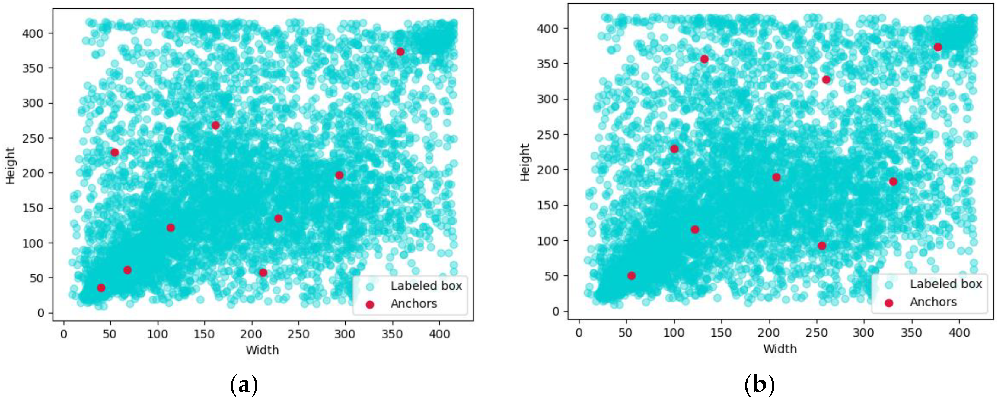
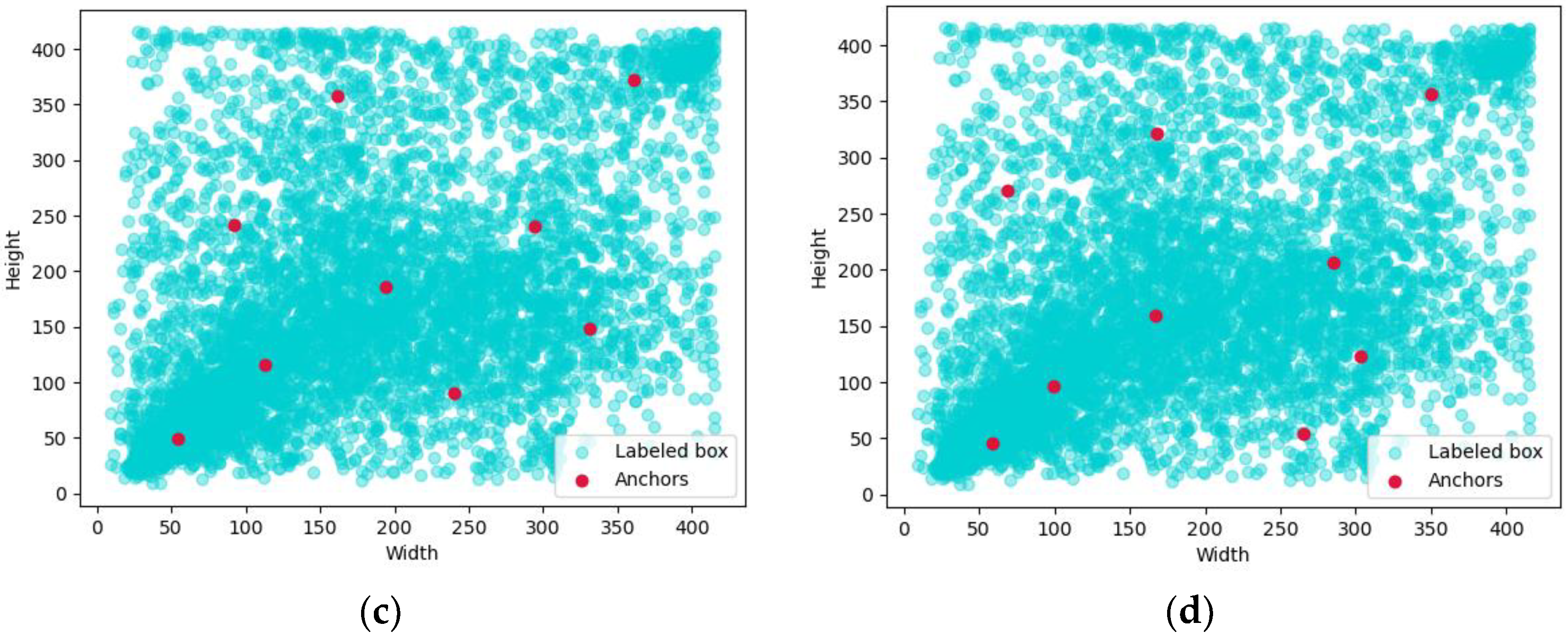
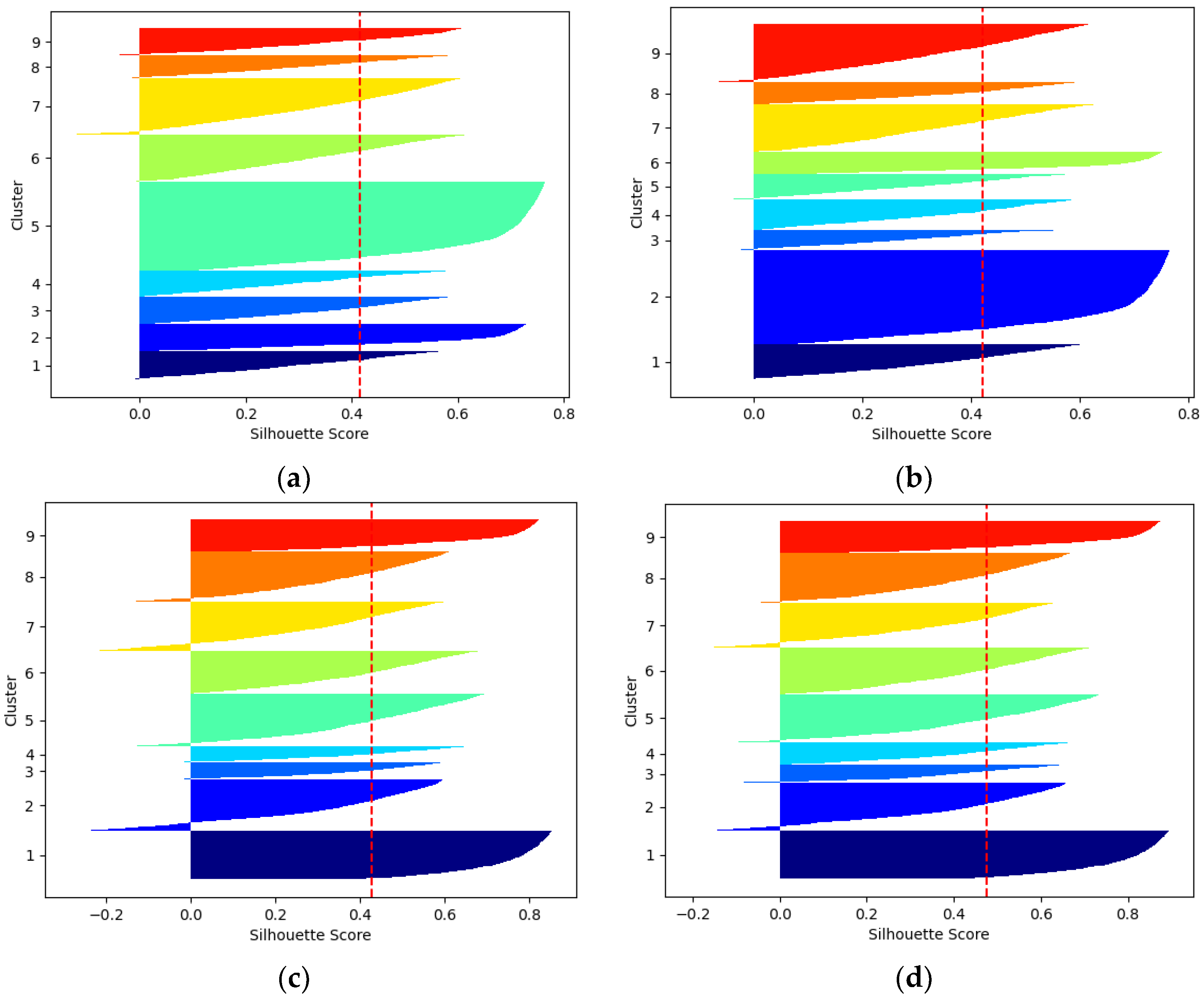
3.1. Optimization of K-Means++ Algorithm Clustering Prior Box

YOLOv3 uses a K-means algorithm to generate a prior box by clustering a marked-ground-truth box, and then takes the size of the prior box as a reference to predict the prediction box of an object. The K-means algorithm first needs to set K clustering centers. For the selection of K, the prior method can be used to set the K value by knowing the prior information of the whole dataset. YOLOv3 predicts feature graphs of three sizes, and each grid of each size has three prior boxes, so the K value is set to 9. The object-detection algorithm based on YOLOv3 requires a large amount of image data, which will generate more marked-ground-truth boxes for clustering, and then more ground-truth boxes with a large size gap will participate in clustering. K-means algorithms are sensitive to outliers in a large amount of data and is easy to generate local-optimal clustering. Therefore, the original K-means algorithm cannot cluster the prior boxes in the dataset well. In view of the problems existing in K-means algorithms, this paper introduces the K-means ++ algorithm and optimizes the K-means++ algorithm to improve the clustering effect of annotated ground-truth boxes in the data, and also provides a good data-clustering foundation for YOLOv3 object detection.

The K-means++ algorithm is mainly used to optimize the selective mode of the initial clustering center. The basis for selecting the initial cluster center is that the distance between the selected points should be as large as possible, so as to ensure that the clustering center will no longer gather in a certain area, which has a better effect on the global clustering of data [22]. The K-means ++ algorithm first randomly selects a sample from the dataset as the initial cluster center, then calculates the distance between other data points and the selected cluster center. The calculation formula is as follows:

$$D\left(x_i\right)=argmin\left|\right|x_i-u_r\left|\right|$$

(1)

where x_i represents each point in the dataset, u_r is the selected cluster center, and r is the selected cluster center. The calculated distance is used to select new data points as the cluster center. The selection basis is that the points with large D(x) have a high probability of being selected as the cluster center. The calculation formula of probability is as follows:

$$P_x=\frac{D{(x)}^2}{{{\displaystyle \sum }}_{x\in X}D{(x)}^2}$$

(2)

where x is the dataset to be clustered.

The distance between the sample point calculated in the above process and the clustering center is the Euclidean distance. In object detection, the purpose of clustering is to make the generated anchor box and the annotated ground-truth box closer. The closer they are, the better the clustering. Therefore, the intersection-over-union (IoU) is used to define a new distance, as shown in Equation (3):

$$D\left(x_i\right)=1-IoU\left(x_i,u_r\right)$$

(3)

where x_i represents each point in the dataset, u_r is the selected cluster center, and r is the number of the selected cluster center. IoU represents the IoU of the two parameters, and the calculation formula is as follows:

$$IoU\left(x_i,u_r\right)=\frac{x_i{\displaystyle \cap }{u}_r}{x_i{\displaystyle \cup }{u}_r}$$

(4)

The above steps must be repeated to select a new cluster centroid until K cluster centroids are selected, and then the selected K cluster centroids must be used to perform the K-means clustering algorithm. At this point, the whole clustering process is completed.

3.2. Fused Attention Mechanism

The convolutional block attention module (CBAM) is a soft attention mechanism lightweight module of the convolution module [23], as shown in Figure 3, in which the channel attention module and spatial attention module process data in the different dimensions respectively. First, the channel attention module is used to compress the spatial dimension of the feature graph, and then the spatial attention module is used to compress the channel dimension. Finally, the convolution operation is used to ensure that the output data dimension is consistent with the input data dimension, so as to complete the construction of the attention mechanism.

3.2.1. Channel Attention Module

In convolutional neural networks, some information is useless relative to the features and information weight can be re-assigned by learning way. The basic idea of the channel attention mechanism is to increase the weight of the effective channel and decrease the weight of the invalid channel, and the most important weight is the attention point of the channel attention mechanism. For image processing tasks, each layer of the convolutional neural network has multiple convolutional kernels. The channel attention mechanism acts on the feature channels corresponding to each convolutional kernel, and each channel has different weights, so that the network pays more attention to the important features and weakens the nonimportant features. As show in Figure 4, the processing flow of the channel attention mechanism is as follows: First, the feature graph of the inputs is subjected to maximum pooling and average pooling operations, through which the loss of feature information can be reduced, and two spatial-information features can be obtained. Then, through a multi-layer perceptron with shared weight value, the output features of multi-layer perceptron are added with the elementwise feature. After the operating of the activation function, the channel attention feature is output. The sigmoid activation function is selected here. The output channel attention feature and the input feature are multiplied by the elementwise feature, and the output feature is taken as the input feature of the spatial-attention module. For the input feature F, its mathematical expression for the channel attention module is as follows:

$$\begin{gathered} M_c\left(F\right)=\sigma \left(MLP\left(Avgpool\left(F\right)+MLP\left(Maxpool\left(F\right)\right)\right)\right) \\ =\sigma (W_1\left(W_0\left(F_{avg}^c\right)\right)+W_1(W_0(F_{max}^c)\left)\right) \end{gathered}$$

(5)

In Equation (5), M_e(F) represents the output of the channel attention module, σ is the sigmoid activation function, W₀ and W₁ are the weight coefficients of the multi-layer perceptron, and $F_{avg}^c$ and $F_{max}^c$ represent the output feature graph after average pooling and maximum pooling.

3.2.2. Spatial Attention Module

The spatial attention module is used to compress the data on the channel and focus on obtaining the effective information in the channel. As shown in Figure 5, after the channel attention mechanism processing is completed, the generated feature graph and the input feature graph are multiplied by the elementwise feature as the input of the spatial attention module, and the input feature graph is pooled in the channel dimension by using the average pooling and maximum pooling methods to generate two feature graphs, which are combined into a new feature map. Because the dimension of the feature graph of the spatial dimension is different from that of the input feature graph, so the convolution operation is needed to keep it consistent, and then activate it through a sigmoid activation function to finally output the spatial attention feature graph. For the input feature F, the mathematical expression of its spatial attention module is shown in Equation (6).

$$\begin{array}{ll}{M}_s(F)& =\sigma (f^{7\times 7}([Avgpool(F);Max(Maxpool(F)]))\\ & =\sigma (f^{7\times 7}([F_{avg}^s;F_{\max }^s]))\end{array}$$

(6)

where $M_s\left(F\right)$ represents the output of the spatial attention module, σ represents the sigmoid activation function, $f^{7\times 7}$ represents the convolution kernel with a size of $7\times 7$, and the $F_{avg}^s$ and $F_{max}^s$ represent the feature graph output after average pooling and maximum pooling respectively.

CBAM integrates channel attention and spatial attention, which not only ensures the acquisition of important channel information, but also ensures the acquisition of important information of characteristic areas. CBAM is widely used in residual network structures, and the YOLOv3 algorithm uses residual network structures to reduce gradient disappearance. Therefore, CBAM is embedded in the YOLOv3 network in this paper. As shown in Figure 6, the embedding of attention mechanisms can be completed by adding a CBAM module behind the residual unit.

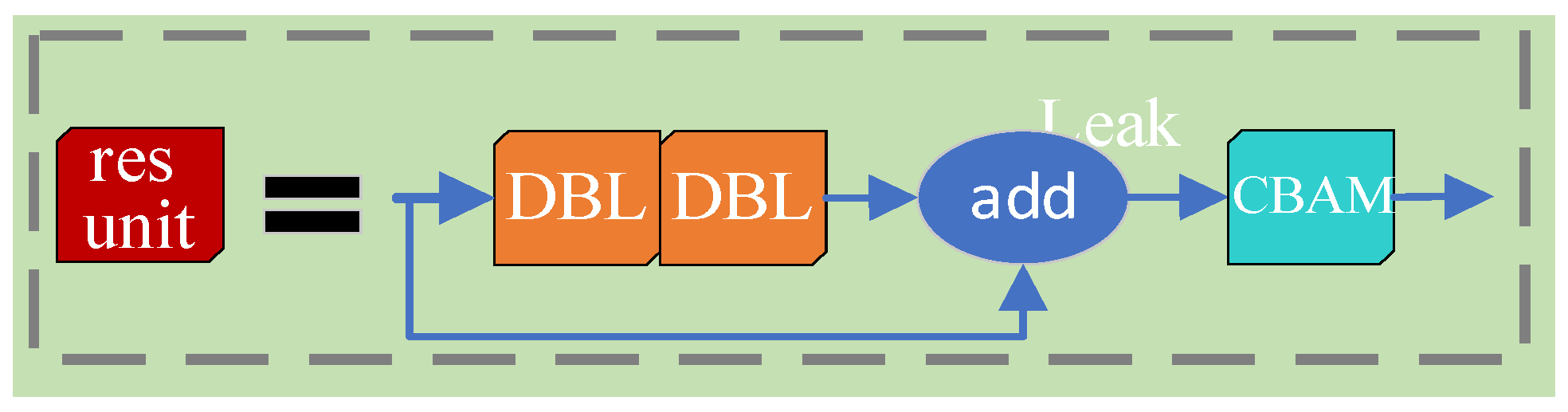
3.3. Improving the Network Structure

The YOLOv3 draws on the principle of feature pyramid structure for reference, integrates the low-level information and the high-level information after up-sampling [24], and makes independent prediction on three feature scales, namely 13 * 13, 26 * 26, and 52 * 52. Many industrial structures, such as the contour of stamping parts, have a large-defect-scale span, including many small objects. For the three characteristic scales of YOLOv3, the amount of information provided by the grid is limited, and the grid is divided by each scale. The detection layer of eight-fold down-sampling is the smallest object layer that can be detected, that is, 52 * 52, which will lead to an inaccurate detection effect of small objects.

In order to further improve the detection ability of the YOLOv3 network for small-object defects of industrial structures, this paper continues to use the FPN principle, shown in Figure 7, to add a scale prediction, and to set the characteristics to four scales, namely, 13 * 13, 26 * 26, 52*52, and 104 * 104. The fourth scale can use the shallow-detail information and deep-feature-semantic information for defecting-object detection, which not only improves the image processing ability of the network, but also enhances the robustness of the network.

Based on the FPN principle and defect image features of industrial structure, this paper proposes a YOLOv3 model with an improved network structure, as shown in Figure 8. The input image passes through the Darknet-53 backbone network that does not have a full connection layer, and the feature graph of four scales is output. The fifth residual block of the backbone network outputs a 32-fold down-sampling feature diagram. After it passes through five DBL convolution layers, one 3 *3 convolution core and one 1 * 1 convolution core, the feature graph of the first scale 13* 13 is acquired. The output of the fifth residual block in the backbone network is a 32-fold down-sampling feature graph. After it passes through five DBL convolution layers, the up-sampling is spliced with the 16-fold down-sampling feature graph output by the fourth residual block in the backbone network as the feature graph of the second scale 26 * 26. The aforementioned 16-fold down-sampling feature graph after splicing is passed through five DBL convolutional layers, and then the up-sampling feature graph is stitched with the eight-fold down-sampling feature diagram output by the third residual block in the backbone network as the feature graph of the third scale 52 * 52. In the same way, the above spliced eight-fold down-sampling feature diagram is passed through five DBL convolution layers, and then the up-sampling feature diagram is stitched with the four-fold down-sampling feature diagram output by the second residual block in the backbone network as the feature graph of the fourth scale 104 * 104. The attention mechanism is used in the network structure, and the CBAM module is embedded behind each residual unit, so that the improved network structure can make full use of the shallow-detail information and high-level semantic information, and improve the detection ability of the network for small objects.

3.4. Optimizing the Loss Function

The loss function plays an important role in object detection. Whether the design of the loss function is reasonable or not is directly related to the training time and detection accuracy of the model [25]. At present, there is no general loss function, and the selection of the loss function requires a comprehensive consideration of factors such as machine learning algorithms, model convergence time, and the confidence of the prediction results. The L2 loss function is used in the YOLOv3 to calculate the loss of the predicted box coordinates. The basic idea of the L2 loss function is to reduce the sum of the squares of the differences between the two data as much as possible. Its mathematical expression is shown in Equation (7):

$$L_2\left(\widehat{y},y\right)={\displaystyle \sum }_{i=0}^m{(y^{\left(i\right)}-{\widehat{y}}^{\left(i\right)})}^2$$

(7)

where $y^{\left(i\right)}$ represents the true value, ${\widehat{y}}^{\left(i\right)}$ represents the estimated value, and m represents the total number of samples.

The robustness of the L2 loss function is poor and mainly reflected in the error squared, which will make the model sensitive to samples with large errors and sacrifice more sample values with small errors for adjustment. The IoU loss function is proposed for object detection, and its evaluation idea is to calculate the intersection ratio between the prediction box and the ground-truth box. The larger the value, the higher the degree of coincidence between the two boxes, and the more similar they are. The mathematical expression for the evaluation of the IoU loss function is as follows:

$$IoU=\frac{\left|A{\displaystyle \cap }B\right|}{\left|A{\displaystyle \cup }B\right|}$$

(8)

In the formula: A and B represent the predicted box and the ground-truth box, respectively. The intersection ratio reflects the detection effect of the predicted box relative to the ground-truth box, but the IoU loss function is insensitive to scale.

Table 1. The loss values of L2, IoU loss, and GIoU loss.

Number/Loss	L2 Loss	IoU Loss	GIoU Loss
a	19.69	0.16	0.07
b	19.69	0.18	0.18
c	19.69	0.29	0.29

demonstrates that when the L2 loss values are the same, the IoU loss values are different, and the GIoU loss values are also very different. It can be clearly seen from the position of the boxes in Figure 9 that the IoU loss values in Figure 9a are significantly less than the IoU loss values in Figure 9c. In Figure 9, the green frames represent the ground-truth boxes, and the red frames represent the prediction boxes. L2. IoU and GIoU are used to calculate the loss.

The IoU loss function also has certain shortcomings that cannot accurately reflect the coincidence degree of the two regions. Figure 10a indicates that the real defect and the prediction defect are close, and Figure 10b indicates that the real defect and the prediction defect are far away from one another. When the prediction box does not coincide with the ground-truth box, the resulting loss is 0, and the network cannot perform parameter learning.

In view of the above problems, we introduce the GIoU (generalized intersection-over-union) loss function [26]. This improved method can solve the problem of the loss function value being 0 when there is no overlap between the prediction box and the ground-truth box, so that the network can carry out back-propagation to optimize the parameters. The GIoU loss is calculated as follows:

$$GIoU=IoU-\frac{\left|C\backslash \left(A{\displaystyle \cup }B\right)\right|}{\left|C\right|}$$

(9)

where A and B represent the prediction box and the ground-truth box, respectively, and C represents the smallest bounding rectangle of the prediction box and the ground-truth box, as shown in the black box line in the Figure 11. IoU represents the intersection-over-union of the prediction box and the ground-truth box.

It can be determined from Equation (9) that the value range of GIoU is (−1,1]. GIoU comprehensively considers the overlapping area and the nonoverlapping area, which can reflect the degree of coincidence between the ground-truth box and the predicted box. The shorter the distance between the two boxes, the closer the value of GIoU is to 0, so this paper defines the GIoU loss function as follows:

$$GIoU loss=1-GIoU$$

(10)

As can be seen from Equation (10), when the GIoU of the prediction box and the ground-truth box is larger, the loss value is smaller, and the network model will perform parameter optimization in the direction of model convergence.

In the dataset of this study, the samples used are stamping parts, which have many small defects. In an image, the areas with defects are used as positive samples, and the areas without defects are used as negative samples. In the actual feature graph output, there are few positive samples of candidate boxes containing defective objects. This will generate a large number of negative-sample candidate boxes, resulting in a class imbalance problem, which will cause the model to fail to learn effective information. The YOLOv3 adopts cross-entropy as a classification loss function. The cross-entropy loss is more sensitive to class imbalance, meaning that when the classification samples are unbalanced, the trained model will be biased to the category with more samples in the training set, so that the multi-classification detection effect of the model is not good.

In view of the above problems, this paper introduces the focal loss function to improve the YOLOv3 confidence loss to solve the problem of class imbalance. The Focal loss formula is as follows:

$$Focal loss=\{\begin{array}{l}-\alpha \left(1-p{)}^{\gamma }\log (p\right)\hspace{1em}y=1\\ -\left(1-\alpha \right)p^{\gamma }\log (1-p)\hspace{1em}y=0\end{array}$$

(11)

where, α is the weight coefficient, which is responsible for adjusting the balance of positive and negative samples; γ is the hyperparameter, which is responsible for adjusting the balance between difficult and easy to classify samples; and y represents whether it is a real label. The results of a large number of experiments prove that when the value of dataset α is 0.5 and the value of γ is 2, the model training effect is the best.

In summary, an improved scheme for integrating GIoU and focal loss is given for the existing problems. The finalloss function of the improved YOLOv3 model in this paper is as follows:

$$\begin{array}{ll}L\mathrm{oss}=& {\displaystyle \sum _{i=0}^{S^2}{\displaystyle \sum _{j=0}^B{I}_{ij}^{obj}}}(1-GIoU)\times (2-w_i\times h_i)-\\ & {\displaystyle \sum _{i=0}^{S^2}{\displaystyle \sum _{j=0}^B{I}_{ij}^{obj}[{\widehat{C}}_i\alpha {(1-C_i)}^{\gamma }\log (C_i)+(1-{\widehat{C}}_i)(1-\alpha ){(C_i)}^{\gamma }\log (1-C_i)]}}-\\ & {\lambda }_{noobj}{\displaystyle \sum _{i=0}^{S^2}{\displaystyle \sum _{j=0}^B{I}_{ij}^{noobj}}}[{\widehat{C}}_i\alpha {(1-C_i)}^{\gamma }\log (C_i)+(1-{\widehat{C}}_i)(1-\alpha ){(C_i)}^{\gamma }\log (1-C_i)]-\\ & {\displaystyle \sum _{i=0}^{S^2}{I}_i^{obj}}{\displaystyle {\sum }_{c\in classes}[{\widehat{P}}_i}(c)\log (P_i(c))+(1-{\widehat{P}}_i(c))\log (1-P_i(c))]\end{array}$$

(12)

where: S is the size of the image being meshed, B is the number of bounding boxes predicted by each grid cell, and ${\lambda }_{noobj}$ is the confidence loss weight when the grid cell does not contain an object. $I_{ij}^{obj}$ and $I_{ij}^{noobj}$ are control terms, indicating whether the jth bounding box of the ith grid cell is responsible for the detection of the current object. When the center point of the object falls on the ith grid cell, and the jth bounding box of the ith grid cell has the largest intersection ratio with the ground-truth box, then $I_{ij}^{obj}$ is 1, and $I_{ij}^{noobj}$ is 0, otherwise $I_{ij}^{obj}$ is 0, and $I_{ij}^{noobj}$ is 1. $I_i^{obj}$ indicates whether the ith grid cell contains an object. $w_i$ and $h_i$ represent the width and height of the ground-truth box, respectively. α is the weight coefficient and γ is a hyperparameter. $C_i$ represents the confidence level of the predicted bounding box, and ${\widehat{C}}_i$ represents the confidence level of the ground-truth box. $P_i\left(c\right)$ represents the class probability of the predicted bounding box, and ${\widehat{P}}_i\left(c\right)$ represents the class probability of the ground-truth box.

4. Experimental Results and Analysis

4.1. Experimental Environment and Model Parameters

The dataset used in this paper contains 3500 contour-defect images of stamping parts, which are divided into five types of defects. The dataset is divided into training sets, validation sets, and test sets in an 8:1:1 ratio. The K-means++ algorithm optimized in this paper is used to cluster prior-bounding boxes, and then the Tensorflow framework is used to build the improved object-detection algorithm. The adaptive moment estimation (Adam) optimizer is used to calculate the gradient to update the parameters in the network. Adam can improve the robustness of the model parameters. Finally, the detection experiment is carried out in the test set of this paper and the results are analyzed.

The experimental environment of the algorithm in this paper includes a hardware environment and a software environment. The program is written in the Python language and accelerated by CUDA. The specific-hardware-environment configuration is shown in

Table 2. The configuration of the experimental environment.

Category	Model/Version
CPU	Intel Xeon CPU E5-2678 v3 @ 2.50 GHz
GPU	NVIDIA GeForce RTX 2080 Ti 11 G
RAM	Samsung RECC DDR4 16 G
SSD	Samsung SSD 860EVO 512 G
Operating system	Ubuntu 18.04
CUDA version	CUDA10.0
cuDNN	cuDNN 7.6
Programming language	Python 3.7

. The hyperparameter setting values required for the network training process are shown in

Table 3. Hyperparameter setting.

Hyperparameter Name	Parameter Value
Learning rate	0.0001
Batch size	16
Weight decay coefficient	0.0005
The number of iterations	100,000

, and the set hyperparameters are suitable for all the target-detection algorithms that need to be compared in this paper. The size of the input image used in the experiment is 416 * 416.

4.2. Analysis of Experimental Result

In order to evaluate the optimized K-means++ algorithm, four K-means series algorithms are used for experiments on the dataset in this study. The receptive fields corresponding to the three feature-graph scales of YOLOv3 are large, medium, and small, respectively. The more the meshes are divided, the smaller the receptive field. The cluster centers are visualized, and Figure 12 is a clustering-effect diagram, wherein Figure 12a shows the K-means algorithm with Euclidean distance as the measurement method, Figure 12b shows the K-means++ algorithm with Euclidean distance as the measurement method, Figure 12c shows the K-means algorithm using the IoU as the measurement method, and Figure 12d shows the K-means++ algorithm using the IoU as the measurement method. The blue points in the figure are the ground-truth boxes marked by the dataset, and the red points denote the cluster center. The abscissa is the width of the cluster box, and the ordinate is the height of the cluster box, in pixels.

Table 4. Cluster prior boxes.

Number of Figure	Feature Graph	Receptive Field	Prior Box
a	$13\ast 13$	Big	$\left(40\times 36\right)$	$\left(68\times 61\right)$	$\left(212\times 58\right)$
	$26\ast 26$	Middle	$\left(54\times 229\right)$	$\left(114\times 122\right)$	$\left(228\times 135\right)$
	$52\ast 52$	Small	$\left(162\times 268\right)$	$\left(293\times 197\right)$	$\left(358\times 374\right)$
b	$13\ast 13$	Big	$\left(55\times 51\right)$	$\left(122\times 116\right)$	$\left(100\times 229\right)$
	$26\ast 26$	Middle	$\left(255\times 93\right)$	$\left(208\times 190\right)$	$\left(132\times 357\right)$
	$52\ast 52$	Small	$\left(330\times 183\right)$	$\left(260\times 327\right)$	$\left(377\times 373\right)$
c	$13\ast 13$	Big	$\left(54\times 49\right)$	$\left(113\times 116\right)$	$\left(240\times 90\right)$
	$26\ast 26$	Middle	$\left(92\times 242\right)$	$\left(194\times 186\right)$	$\left(331\times 149\right)$
	$52\ast 52$	Small	$\left(162\times 358\right)$	$\left(294\times 240\right)$	$\left(361\times 372\right)$
d	$13\ast 13$	Big	$\left(59\times 46\right)$	$\left(99\times 97\right)$	$\left(265\times 54\right)$
	$26\ast 26$	Middle	$\left(69\times 271\right)$	$\left(167\times 159\right)$	$\left(303\times 123\right)$
	$52\ast 52$	Small	$\left(168\times 322\right)$	$\left(285\times 207\right)$	$\left(350\times 357\right)$

shows the specific values corresponding to the cluster centers in Figure 12. The numbers a, b, c, and d correspond to the above four schemes.

In this study, the contour coefficient is used to evaluate the quantitative effect of the above experiments, and the contour silhouette diagram is drawn, as shown in Figure 13. Figure 13a shows the K-means algorithm with Euclidean distance as the measurement method, Figure 13b shows the K-means++ algorithm with Euclidean distance as the measurement method, Figure 13c shows the K-means algorithm with the IoU as the measurement method, and Figure 13d shows the K-means++ algorithm with the IoU as the measurement method. The abscissa in the figure is the value of the contour coefficient. The larger the contour coefficient value, the more appropriate the clustering effect is. The ordinate represents the category of clustering, meaning the nine clustering prior boxes that the YOLOv3 needs to choose. According to the contour coefficient of all the sample points, the silhouette image in the figure is drawn. The larger the vertical height of the silhouette image occupies, the more samples there are in the current category. The red-dotted line in the figure represents the cluster average contour coefficient. When there are more silhouette images in the figure, the horizontal width exceeding the red dotted line can be considered to be suitable for clustering; the larger the value of the cluster average silhouette coefficient, the better the clustering effect.

It can be seen from Figure 13 that most of the values of the four silhouette images are positive, so the clustering is effective. It can be seen from

Table 5. Comparison of clustering effects.

Number of Figure	Clustering Method	Measurement Method	Number of Clustering Centers	Value of Average Contour Coefficient
a	K-means	Euclidean distance	9	0.41
b	K-means++	Euclidean distance	9	0.42
c	K-means	IoU	9	0.43
d	K-means++	IoU	9	0.48

that the clustering average contour coefficients are all greater than 0.4. For the dataset in this paper, the K-means++ algorithm is better than the K-means algorithm in the same measurement method, and the clustering algorithm using IoU as the measurement method is used. The clustering effect is better than the Euclidean distance, and the vertical height of the silhouette image using IoU as the measurement method is more average. On the premise that the samples of various defect types in the dataset are balanced, it is also reasonable for the data to be clustered more evenly. The improved K-means++ algorithm, meaning the K-means++ algorithm that uses IoU as the unit of measurement, has the highest average silhouette coefficient of 0.48, so this paper adopts the K-means++ algorithm combined with IoU as the clustering algorithm of the prior box.

The improvement effect in the model-training process can be evaluated by observing the convergence speed of different algorithm models. The faster the loss value decreases, the faster the model converges. In Figure 14, YOLOv3-CBAM represents the YOLOv3 algorithm embedded in CBAM, YOLOv3-Loss represents the YOLOv3 algorithm that improves the loss function, YOLOv3-4L represents the YOLOv3 algorithm that adds the fourth scale, and YOLOv3-ALL is the YOLOv3 algorithm fusing all the above improvement points. The YOLOv3-ALL model proposed in this paper basically converges after 90,000 iterations. The loss value at 100,000 iterations is 2.78, while the loss value of the unimproved YOLOv3 model is 3.74, and it can also be seen from the image that the loss value of the YOLOv3-ALL model decreases faster, indicating that the YOLOv3-ALL model converges more easily and the curve fluctuation amplitude is smaller, while the unimproved YOLOv3 model curve fluctuation is larger, which also shows that the improved loss function designed in this study is more appropriate, so that the predicted value is closer to the true value faster.

Comparing the data in

Table 6. Experimental performance evaluation.

Algorithm Name	Pit (AP%)	Patches (AP/%)	Scratches (AP/%)	Crazing (AP/%)	Concave (AP/%)	mAP (%)
YOLOv3	76.94	65.46	54.74	30.32	21.97	49.89
YOLOv3-CBAM	80.36	67.39	56.16	31.23	23.41	51.71
YOLOv3-Loss	85.21	71.46	72.36	43.45	42.53	63.00
YOLOv3-4L	84.69	75.23	73.63	51.16	40.19	64.98
YOLOv3-ALL	94.85	82.58	78.11	68.54	51.15	75.05

, it can be seen that in the detection of five kinds of stamping-contour defects, the AP value of the algorithm in this paper for the five types of defect detection results for pit, patches, scratches, crazing, and concave are 94.85%, 82.58%, 78.11%, 68.54%, and 51.15%, respectively, while the AP values of the unimproved YOLOv3 model for the five types of defect detection results are 76.94%, 65.46%, 54.74, 30.32% and 21.97%, respectively. The YOLOv3-ALL model in this paper performs better than the unimproved YOLOv3 model, and the detection accuracy for pit defects is up to 94.85%, which also shows that the improvement of the network structure in this paper improves the network’s ability to detect small objects.

As can be seen from Table 6, the mAP value of the YOLOv3-ALL algorithm reaches 75.05%, while the mAP value of the unimproved YOLOv3 algorithm is 49.89%. In general, the mAP value of the novel YOLOv3 algorithm increases by 25.16%, which shows that the algorithm in this paper is better than the traditional YOLOv3 algorithm in all categories of contour-defect detection for stamping parts. Among these types of defects, cracks and pits are typically small and difficult-to-detect objects. Since the algorithm in this paper adds the feature-graph detection of the fourth scale, the detection effect is significantly improved. The obvious improvement also shows that the algorithm in this paper has superior performance in the feature detection of various defect categories. As can be seen from

Table 7. Time comparison of detection by different models.

Algorithm Type	Test Pictures (piece)	Total Time Taken (ms)	Average Detection Time (ms)
YOLOv3	300	9713	32
YOLOv3-ALL	300	11628	39

, the average detection time of the YOLOv3-ALL algorithm in this paper is 39 ms, which is 7 ms slower than the traditional YOLOv3 algorithm, but it can also meet the real-time requirements in an industrial environment.

The detection results of the test set using the YOLOv3-ALL algorithm and the YOLOv3 algorithm, respectively, are shown in Figure 15 and Figure 16. In the two figures, Figure 15a and Figure 16a show the stamping-part contour-defect sample with pit defects, and are marked with cyan boxes and labed pit; Figure 15b and Figure 16b represent the stamping-part contour-defect sample with patch defects, and are marked with dark blue boxes and labeled patch; Figure 15c and Figure 16c represent the stamping-part contour-defect sample with scratch defects, and are marked with green boxes and labeled scratches; Figure 15d and Figure 16d show a sample of stamping-contour defects with crack defects and are marked with orange boxes and labeled crazing; and Figure 15e shows the sample of stamping-contour defects with concave defects, and are marked with pink boxes and labeled concave. It can be seen from the two sets of figures that both algorithms can detect various types of defects, but the algorithm of the YOLOv3-ALL in this paper performs well in the test results of various defects, and the detection accuracy is higher than that of YOLOv3. Furthermore, it also has a better detection effect when there are multiple stamping-contour defects in the same sample.

5. Conclusions

In order to achieve efficient and accurate detection of contour defects for industrial parts, we propose a novel YOLOv3 defect-detection algorithm YOLOv3-ALL, and tested it on a test dataset. Experimental results show that this algorithm has good real-time detection efficiency and high detection accuracy, and provides theoretical and technical support for on-line defect detection of industrial structural parts. Due to the limitations of the experimental environment and industrial environment, there are fewer types and lower numbers of stamping contour defects collected in this study, so our algorithm in this paper still has room for improvement in detection accuracy. Our experiments were all carried out on a PC, and the trained models took up a lot of disk space. In the future, knowledge distillation or model pruning can be considered to compress the models so that they can be applied to embedded devices.

References

1. Luo, Q.; Fang, X.; Liu, L.; Yang, C.; Sun, Y. Automated Visual Defect Detection for Flat Steel Surface: A Survey. IEEE Trans. Instrum. Meas. 2020, 69, 626–644. [Google Scholar] [CrossRef] [Green Version]
2. Czimmermann, T.; Ciuti, G.; Milazzo, M.; Chiurazzi, M.; Roccella, S.; Oddo, C.M.; Dario, P. Visual-based defect detection and classification approaches for industrial applications—A survey. Sensors 2020, 20, 1459. [Google Scholar] [CrossRef] [PubMed] [Green Version]
3. Zhang, H.; Jing, H.; Chen, T.; Zhang, Y.; Pu, W. Partial Application of Defect Detection in Industry. Int. Core J. Eng. 2021, 7, 144–147. [Google Scholar]
4. Neogi, N.; Mohanta, D.K.; Dutta, P.K. Defect detection of steel surfaces with global adaptive percentile thresholding of gradient image. J. Inst. Eng. (India) Ser. B 2017, 98, 557–565. [Google Scholar] [CrossRef]
5. Haoran, G.; Wei, S.; Awei, Z. Novel defect recognition method based on adaptive global threshold for highlight metal surface. Chin. J. Sci. Instrum. 2017, 38, 2797–2804. [Google Scholar]
6. Wang, Z.; Zhang, C.; Li, W.; Qian, J.; Tang, D.; Cai, B.; Chang, Y. Cathodic Copper Plate Surface Defect Detection based on Bird Swarm Algorithm with Chaotic Theory. J. Image Graph. 2020, 25, 697–707. [Google Scholar]
7. Cao, G.; Ruan, S.; Peng, Y.; Huang, S.; Kwok, N. Large-Complex-Surface Defect Detection by Hybrid Gradient Threshold Segmentation and Image Registration. IEEE Access 2018, 6, 36235–36246. [Google Scholar] [CrossRef]
8. Shi, T.; Kong, J.; Wang, X.; Liu, Z.; Zheng, G. Improved Sobel Algorithm for Defect Detection of Rail Surfaces with Enhanced Efficiency and Accuracy. J. Cent. South Univ. 2016, 23, 2867–2875. [Google Scholar] [CrossRef]
9. Zhou, S.Y. Research on Detecting Method for Image of Surface Defect of Steel Sheet Based on Visual Saliency and Sparse Representation. Ph.D. Thesis, Huazhong University of Science and Technology, Wuhan, China, 2017. [Google Scholar]
10. Huang, Q.; Zhang, H.; Zeng, X.; Huang, W. Automatic Visual Defect Detection Using Texture Prior and Low-Rank Representation. IEEE Access 2018, 6, 37965–37976. [Google Scholar] [CrossRef]
11. Wang, J.; Li, Q.; Gan, J.; Yu, H.; Yang, X. Surface Defect Detection via Entity Sparsity Pursuit With Intrinsic Priors. IEEE Trans. Ind. Inform. 2020, 16, 141–150. [Google Scholar] [CrossRef]
12. Perez, H.; Tah, J.H.; Mosavi, A. Deep learning for detecting building defects using convolutional neural networks. Sensors 2019, 19, 3556. [Google Scholar] [CrossRef] [PubMed] [Green Version]
13. Zhou, H.; Zhuang, Z.; Liu, Y.; Liu, Y.; Zhang, X. Defect classification of green plums based on deep learning. Sensors 2020, 20, 6993. [Google Scholar] [CrossRef] [PubMed]
14. Jiao, L.; Zhang, F.; Liu, F.; Yang, S.; Li, L.; Feng, Z.; Qu, R. A survey of deep learning-based object detection. IEEE Access 2019, 7, 128837–128868. [Google Scholar] [CrossRef]
15. Felzenszwalb, P.; McAllester, D.; Ramanan, D. A discriminatively trained, multiscale, deformable part model. In Proceedings of the 2008 IEEE Conference on Computer Vision and Pattern Recognition, Anchorage, AK, USA, 1–8 June 2008. [Google Scholar]
16. Girshick, R.; Iandola, F.; Darrell, T.; Malik, J. Deformable part models are convolutional neural networks. In Proceedings of the IEEE Conference on Computer Vision and Pattern Recognition, Boston, MA, USA, 7–12 June 2015; pp. 437–446. [Google Scholar]
17. He, K.; Zhang, X.; Ren, S.; Sun, J. Spatial Pyramid Pooling in Deep Convolutional Networks for Visual Recognition. IEEE Trans. Pattern Anal. Mach. Intell. 2015, 37, 1904–1916. [Google Scholar] [CrossRef] [PubMed] [Green Version]
18. Redmon, J.; Divvala, S.; Girshick, R.; Farhadi, A. You only look once: Unified, real-time object detection. In Proceedings of the IEEE Conference on Computer Vision and Pattern Recognition, Las Vegas, NV, USA, 27–30 June 2016; pp. 779–788. [Google Scholar]
19. Redmon, J.; Farhadi, A. YOLO9000: Better, faster, stronger. In Proceedings of the IEEE Conference on Computer Vision and Pattern Recognition, Honolulu, HI, USA, 21–26 July 2017; pp. 7263–7271. [Google Scholar]
20. Seferbekov, S.; Iglovikov, V.; Buslaev, A.; Shvets, A. Feature pyramid network for multi-class land segmentation. In Proceedings of the IEEE Conference on Computer Vision and Pattern Recognition Workshops, Salt Lake City, UT, USA, 18–22 June 2018; pp. 272–275. [Google Scholar]
21. Redmon, J.; Farhadi, A. Yolov3: An incremental improvement. arXiv 2018, arXiv:1804.02767. [Google Scholar]
22. Xu, Y.; Zhang, K.; Wang, L. Metal Surface Defect Detection Using Modified YOLO. Algorithms 2021, 14, 257. [Google Scholar] [CrossRef]
23. Woo, S.; Park, J.; Lee, J.Y.; Kweon, I.S. Cbam: Convolutional block attention module. In Proceedings of the European Conference on Computer Vision (ECCV), Munich, Germany, 8–14 September 2018; pp. 3–19. [Google Scholar]
24. Lin, T.Y.; Dollár, P.; Girshick, R.; He, K.; Hariharan, B.; Belongie, S. Feature pyramid networks for object detection. In Proceedings of the IEEE Conference on Computer Vision and Pattern Recognition, Honolulu, HI, USA, 21–26 July 2017; pp. 2117–2125. [Google Scholar]
25. Qianhui, Y.; Changlun, Z.; Qiang, H.; Hengyou, W. Research Progress of Loss Function in Object Detection. Comput. Sci. Appl. 2021, 11, 2836–2844. [Google Scholar]
26. Rezatofighi, H.; Tsoi, N.; Gwak, J.; Sadeghian, A.; Reid, I.; Savarese, S. Generalized intersection over union: A metric and a loss for bounding box regression. In Proceedings of the IEEE/CVF Conference on Computer Vision and Pattern Recognition, Long Beach, CA, USA, 15–20 June 2019; pp. 658–666. [Google Scholar]
Figure 1. YOLOv3 network structure.
Processes 10 00701 g001
Figure 2. Feature pyramid network schematic diagram.
Processes 10 00701 g002
Figure 3. CBAM network structure.
Processes 10 00701 g003
Figure 4. Channel attention module.
Processes 10 00701 g004
Figure 5. Spatial attention module.
Processes 10 00701 g005
Figure 6. CBAM added to the residual unit.
Processes 10 00701 g006
Figure 7. Improved feature fusion network.
Processes 10 00701 g007
Figure 8. Improved YOLOv3 network structure.
Processes 10 00701 g008
Figure 9. The comparison of L2 loss, IoU loss, and GIoU loss. (a)The loss values of L2. (b) The loss values of IoU. (c) The loss value of GIoU.
Processes 10 00701 g009
Figure 10. Comparison of the distance between the prediction box and ground-truth frame. (a) The real defect is close to the predicted defect. (b) The real defect is far from the predicted defect.
Processes 10 00701 g010
Figure 11. The smallest bounding rectangle C of GIoU.
Processes 10 00701 g011
Figure 12. Clustering effect of different algorithms: (a) K-means algorithm with Euclidean distance; (b) K-means++ algorithm with Euclidean distance; (c) K-means algorithm with IoU; (d) K-means++ algorithm with IoU.
Processes 10 00701 g012aProcesses 10 00701 g012b
Figure 13. The contour silhouette image of clustering algorithm. (a) K-means algorithm with Euclidean distance; (b) K-means++ algorithm with Euclidean distance; (c) K-means algorithm with IoU; (d) K-means++ algorithm with IoU.
Processes 10 00701 g013
Figure 14. Comparison of four loss function curves. (a) The loss function values of YOLOv3 and YOLOv3-ALL; (b) The loss function values of YOLOv3-ALL, YOLOv3-CBMA, YOLOv3-4L, and YOLOv3-Loss.
Processes 10 00701 g014
Figure 15. The test results of YOLOv3-ALL. (a) The defects of pit. (b) The defects of patch. (c) The defects of scratch. (d) The defects of crack. (e) The defects of pit.
Processes 10 00701 g015
Figure 16. The test results of YOLOv3. (a) The defects of pit. (b) The defects of patch. (c) The defects of scratch. (d) The defects of crack. (e) The defects of pit.
Processes 10 00701 g016