Valuation of Climate Performance of a Low-Tech Greenhouse in Costa Rica

Abstract

The expansion of protected agriculture has technological, climatic, and topographic limitations. The agricultural regions of Costa Rica use the greenhouse concept and adapt it to its conditions. The objective of this work was to describe the variation in temperature and humidity in a greenhouse ventilated passively and on land with a more than 45% slope. To evaluate the environment inside the greenhouse, temperature and humidity variations were measured with a weather station installed outside of the greenhouse to measure the external environment. Inside the greenhouse, 17 sensors were placed to measure the temperature (T) and relative humidity (RH). During data recording inside the greenhouse, tomato crops were in the fruit formation stage, and pepper was less than one week old. Six scenarios were tested to determine the air temperature and humidity dynamic under different climatic conditions. An evaluation of the greenhouse environment was carried out employing an analysis of variance of temperature and RH to establish if there are significant differences in the direction of the slope of the cross-section. The uniformity of temperature and RH do not present stratifications derived from wind currents that can affect the effective production of these crops.

1. Introduction

Advances in technology have brought solutions in regions with adverse climatic conditions. The objective is to produce crops with the efficient use of natural resources to avoid fossil energy to improve the quality and yield of crops all year long. These structures have had to evolve to answer each condition and necessity. Tropical conditions imply high humidity, and topographic restrictions mean that greenhouses must be built on a non-plane surface, in which there are hardly any management systems for climate control.

Passive ventilation is used in greenhouses to evacuate heat excess, which occurs at specific times due to insolation, which is characterized as a function of geographic localization (latitude) and topographic condition (high over sea level). In a greenhouse, windows in different positions (roof, lateral or frontal) are used to maintain an adequate environment for crops. The density of crops and the design of the greenhouse also contribute to air renovation and, consequently, better climatic conditions [1,2,3].

Greenhouses in Costa Rica have slowly increased functional crop production: in 2010, 681 greenhouses covered an area of 688.23 hectares. Most of the existing greenhouses are artisanal; therefore, there are problems regarding climate control of the variables used to obtain better environmental conditions for crops in greenhouses, affecting the production quality [4,5,6]. For this reason, natural ventilation has become one of the most important phenomena for managing the environmental conditions inside the structure. Through the airflows generated by the difference in pressures, it is possible to regulate temperature (T°) and relative humidity (RH) surplus into the greenhouse [7,8].

Greenhouse evolution and the prospect of achieving better environmental conditions are central to knowledge concerning climate condition [9,10]. The condition of crops within a greenhouse depends a combination of climate factors such as radiation, and, consequently, temperature (T °C), relative humidity (RH %), carbon dioxide (CO₂, ppm), vapor pressure deficit (VPD, Pa), etc. each of which determine the condition of crops along their lifecycle [11,12]. In addition to agronomic conditions, auxiliary climatic systems are also defined as a function of energy variables such as temperature and relative humidity [13].

Climatic restrictions for the establishment and operation of greenhouses were normally exposed and fixed with natural or mechanical ventilation systems [9]. Even though other restrictions exist for the expansion of protected agriculture, such as those with topographic land characteristics, these have not been documented. In specific regions of Costa Rica, they are typically used for agricultural production in an irregular topographic land as an optional crop production system under controlled environments; however, if the optimum conditions have not existed, the adaptation can be expensive and prevent the benefits of its use. Such an aspect can become one of the most delimitated factors when a project to build such a greenhouse is undertaken.

Throughout the world it is common to build greenhouses on a plane surface to facilitate agronomic labour. The idea of the use of a sloping greenhouse, in general, was to avoid, per se, problems such as the concentration of water and nutritive solution in the irrigation systems and non-uniformity concentration of heat and moisture. However, there are few studies concerning the environmental performance of greenhouses in hillside regions and the subject is relatively unknown [6,14].

Natural ventilation is a prominent phenomenon responsible for managing the environmental conditions inside greenhouses. The airflows generated by the difference in thermal or wind pressure regulate the thermal and humidity excesses inside a greenhouse [7,15]. Moreover, these same airflows are responsible for exchanging air between the interior and exterior, improving thermal and CO₂ conditions [16].

The study of natural ventilation in agricultural structures is not a simple activity to perform experimentally. Although the development of climate monitoring equipment allows the study of air flows through sonic anemometry and temperature sensors, anemometers only allow estimating the velocity and direction of airflow at a spatial point for a given time [17,18,19].

The objective of this work was to describe the variation in temperature and humidity in a greenhouse ventilated passively and with a land slope of more than 45%. In addition to this analysis, with the climatic information and analysis, in future investigations, the use of CFD simulation will be possible to contribute to achieving the design and climate management of this kind of greenhouse.

2. Materials and Methods

2.1. Study Area Localization Zone

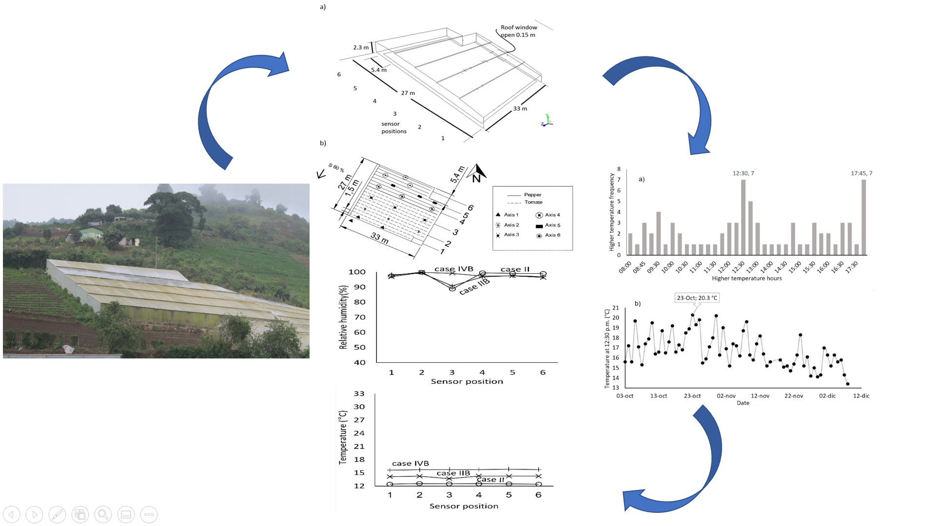
The greenhouse used in this study is located at Zarcero, in the province of Alajuela (10°14′19.2′′ N, 84°22′58.8′′ W) with an altitude of 1875 masl built on land with a more than 45% slope, which represents the local characteristics in the Alajuela region under tropical conditions for cultivation [20,21]. According to the Köppen–Geiger climate classification, the predominant climate in the region is classified as Aw. The average annual temperature ranges from 22.3 °C, and an average rainfall of 2069 mm has been recorded. The greenhouse used was built by hand and has an area of 891 m², covered with a low-density polyethylene and insect-proof screen on the side and roof opening (Figure 1a).

For data acquisition of climatic variables, a weather station (Vantage Pro2 Plus, Davis Instruments, Hayward, CA, USA) was installed 50 m northwest of the greenhouse location and 1.5 m high to record the environmental variables of solar radiation, RH, and temperature every 15 min (

Table 1. Range of measured and precision of climate sensors.

Sensor	Range of Work	Precision
Temperature	−40 to 65 °C	±0.5 °C
Relative Humidity	1 to 100%	±3% y ±4% over 90%
Radiation	0 to 1800 W m−2	±5%
Wind velocity	1 to 80 ms−1	±5 ms−1
Wind directions	16 points of compass	±5

). In the greenhouse, 17 Temperature (°C) and RH (%) sensors (HOBO U10/003, Onset Computer Corporation, Bourne, MA, USA) were installed 1.65 m from the floor, divided into three perpendicular blocks and six lines parallel to the slope to analyse the differences in the slope and cross-section every 5 min (Figure 1b).

The monitoring period was from 2 October 2014 to 8 December 2014, using the WeatherLink© for Vantage Pro2TM (Davis Instrument, CA, USA) and HOBO(HOBO Inc., Bourne, MA, USA) version 3.7.3 computer package.

The outdoor weather station was 1.5 m above the ground. The sensors in the indoor greenhouse were placed at 1.65 m to allow them to record the air temperature data without the influence of the crops. The shield of the sensors was appropriate to the climate station.

Data recording and storage were recorded every 15 min for the weather station and every 5 min on the OOBSet HOBO sensors. The monitoring period was from 2 October 2014 to 8 December 2014, using the WeatherLink© computing package for Vantage Pro2TM and HOBO W version 3.7.3. The six lines of the sensor (axes) were separated, each 5.6 m, in the other directions (33 m); the separation was 10 m from the centre of the greenhouse (Figure 1).

2.2. Sampling and Data Acquisition

For the analysis of temperature and RH behaviour, the information from the sensors was grouped by axes and blocks, shown in Figure 1 in two intervals: daytime from 6:00 a.m. to 5:45 p.m., and night-time from 6:00 p.m. to 5:45 a.m. from 2 October to 8 December 2014, to allow a comparison between axes and to analyze the differences in the slope and between blocks in the cross-section to the slope.

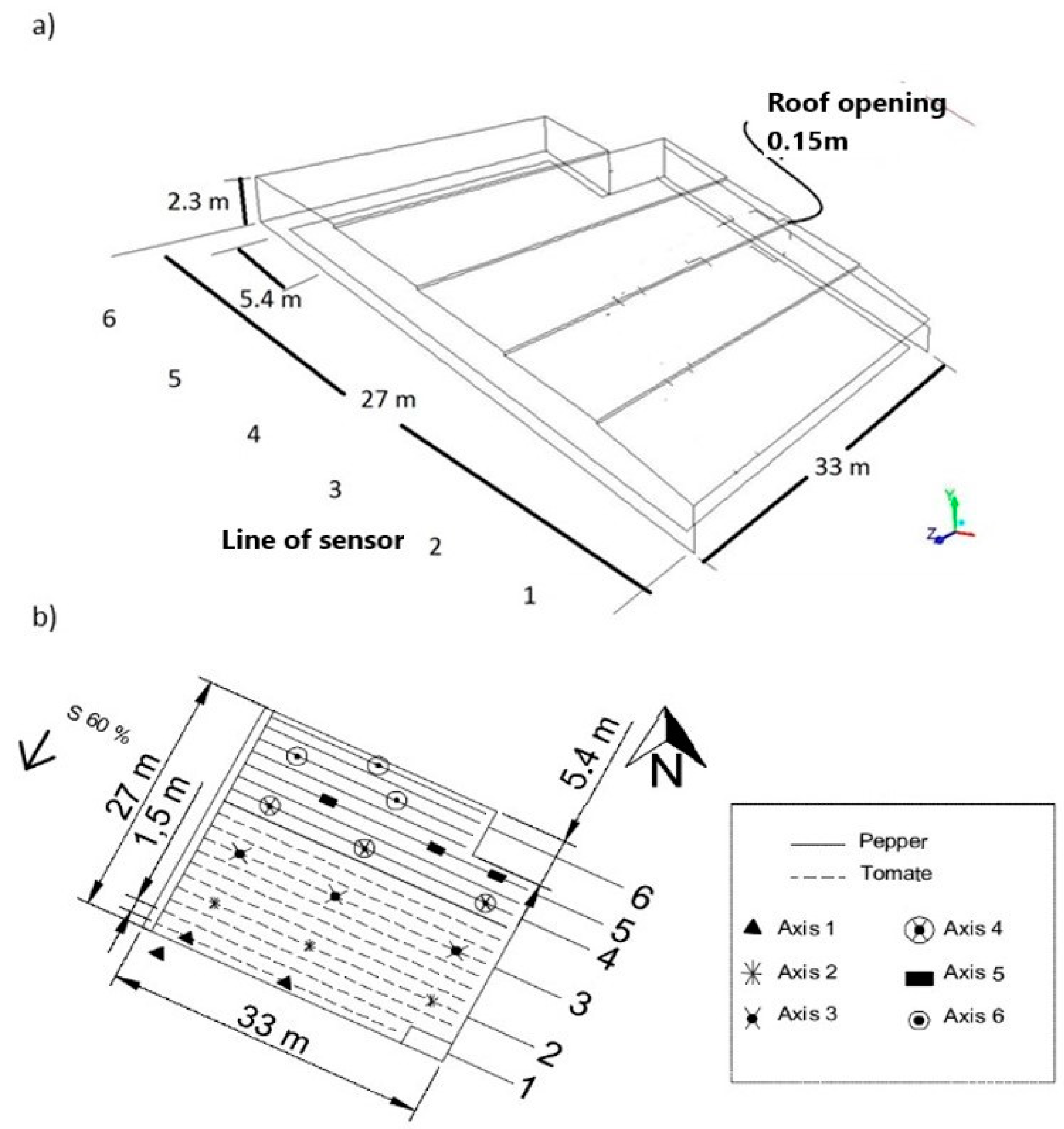
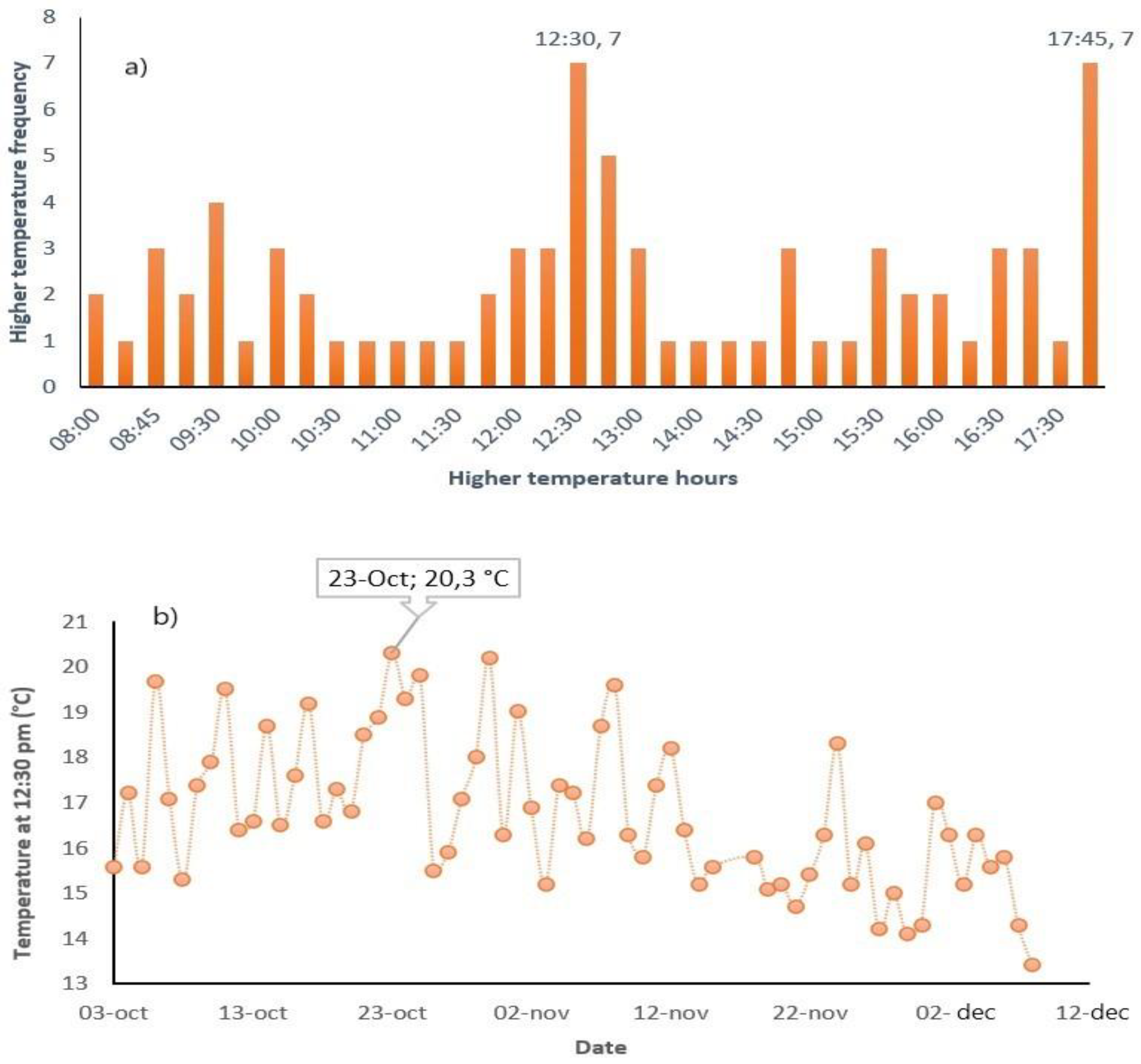
In the first case, the frequency of hours with higher temperatures in the time interval during the sensor monitoring period was considered (Figure 2a). The chosen time was 12:30 p.m. instead of 5:45 p.m., as the maximum temperatures at 5:45 p.m. were during December, the month where the daily temperatures are the lowest of the year. The results showed that the highest temperature (20.3 °C) was at 12:30 p.m. on 23 October (Figure 2b).

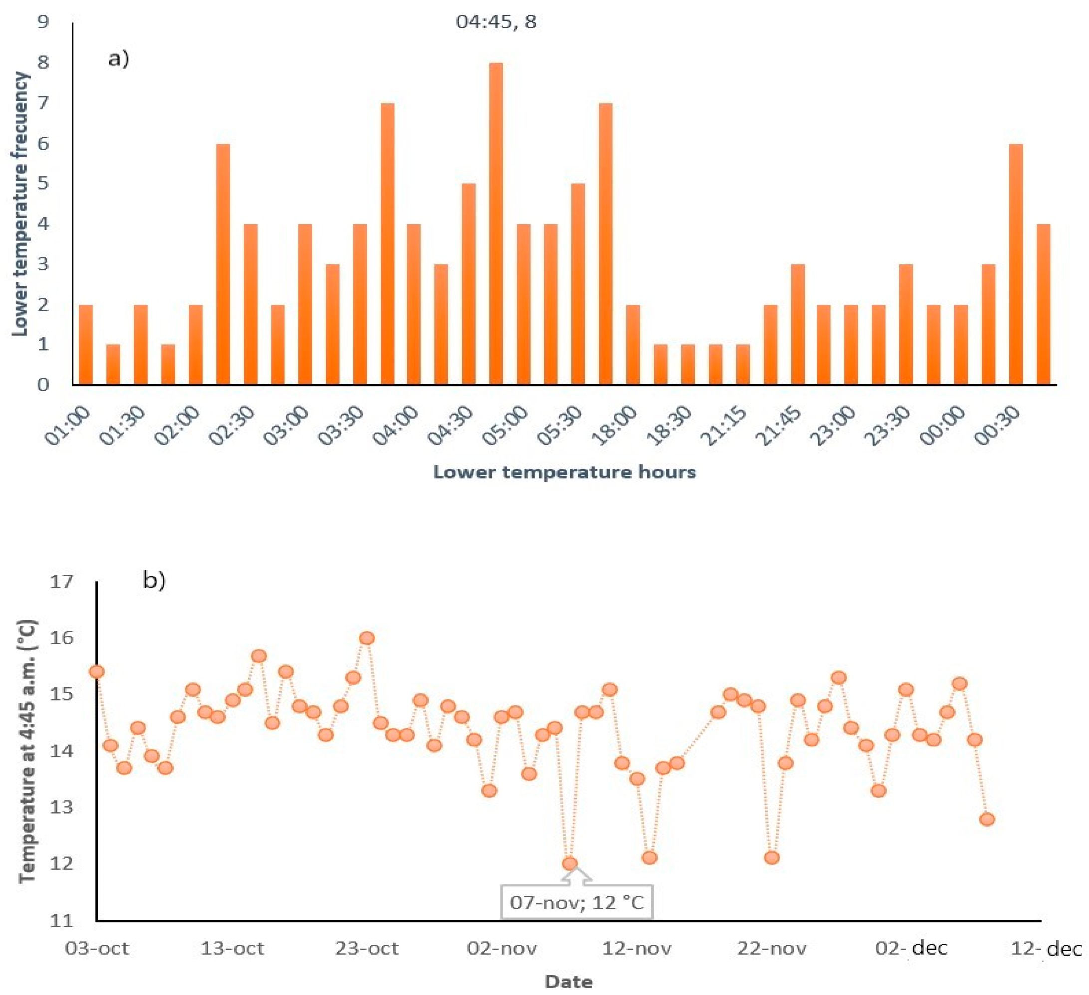
The frequency of hours with the lowest temperature in the night interval during the sensor monitoring period was considered for the second case. The highest frequency of minimum recorded data was at 4:45 h. The date with the lowest temperature occurred on 7 November at 4:45 a.m. (12.0 °C) (Figure 3).

To broaden the view of the environmental behaviour of the greenhouse, two random dates were selected so that the analysis included at least one day of each month registered. The days selected were 6 October and 6 December 2014. Each day was evaluated considering the two hours evaluated in cases I and II.

Table 2. Values of climatic variables considered in the case studies.

Case	Date	Time (h)	Temperature (°C)	RH (%)	Wind
					Velocity (m/s)	Predominant Direction
I	23 October	12:30	20.3	85	2.2	SW
II	07 November	04:45	12.0	97	0.4	SW
IIIA	06 October	12:30	19.7	87	1.8	SE
IIIB	06 October	04:45	14.4	95	0.9	W
IVA	06 December	12:30	15.8	95	0.9	SE
IVB	06 December	04:45	15.2	96	0.9	NW

shows the weather conditions recorded by the weather station of the six case studies (half-hourly average values used as an initial boundary condition of the computational model for each evaluated case).

To determine whether there are spatial variations in temperature and relative humidity in the greenhouse, an analysis of variance was performed using Tukey’s method and orthogonal contrasts, as well as the values of temperature and RH during the study days analysed in the direction of the slope (between axes) and the transverse direction (between blocks).

3. Results and Discussion

3.1. Statistical Analysis of Experimental Data

The analysis of variance for temperature and RH of the scenario is presented in

Table 3. Tukey’s method for the case I analyses the temperature and relative humidity variance between axes and blocks.

Temperature (°C)					RH (%)
Axis	Average	n	E.E.		Axis	Average	n	E.E.
1	30.59	2	1.01	a	1	50.06	1	5.74	a
2	30.71	3	0.82	a	2	49.55	3	3.31	a
3	31.53	3	0.82	a	3	49.72	2	4.06	a
4	32.48	3	0.82	a	4	42.13	2	4.06	a
5	32.55	3	0.82	a	5	43.53	3	3.31	a
6	31.8	3	0.82	a	6	47.36	3	3.31	a
Temperature (°C)					RH (%)
Block	Average	n	E.E.		Block	Average	n	E.E.
A	31.69	5	0.67	a	A	44.97	4	2.89	a
B	31.68	7	0.57	a	B	47.02	6	2.36	a
C	31.64	5	0.67	a	C	48.27	4	2.89	a

Means with a joint letter are not significantly different (p > 0.05).

. It is observed that there is no significant difference for both temperature and RH in the axes or blocks. The same happened for cases II, IIIA, IIIB, and IVB.

Table 4. Tukey’s method for the case IVA analyses the temperature and relative humidity variance between axes and blocks.

Temperature (°C)					RH (%)
Axis	Average	n	E.E.		Axis	Average	n	E.E.
1	22.04	2	0.55	a	1	68.56	1	4.41	a
2	23.11	3	0.45	ab	2	66.88	3	3.6	a
3	23.72	3	0.45	ab	3	65.85	2	4.41	a
4	24.12	3	0.45	ab	4	59.74	2	3.6	a
5	25.18	3	0.45	a	5	58.98	3	3.6	a
6	24.88	3	0.45	a	6	60.07	3	3.6	a
Temperature (°C)					RH (%)
Block	Average	n	E.E.		Block	Average	n	E.E.
A	23.88	5	0.58	a	A	59.35	4	3.24	a
B	24.01	7	0.49	a	B	63.37	6	2.45	a
C	23.92	5	0.58	a	C	64.97	4	2.9	a

Means with a joint letter are not significantly different (p > 0.05).

shows the results of the analysis of variance for the IVA case. It is highlighted that only for this case, there are significant differences between axis 1 and axis 5, and axis 1 with axis 6. On the other hand, the values of the RH mean between axes and blocks did not present statistically significant differences [20].

From the above results, it can be concluded that there is not always a statistically representative thermal difference in the direction of the slope in the greenhouse built on a hillside. In none of the cases analysed were statistically representative differences of RH obtained in the direction of the slope. Furthermore, in the transverse direction of the slope, a statistically representative difference was obtained for temperature or RH in no case.

3.2. Temperature and RH Variation between Axes and between Blocks (Day Time)

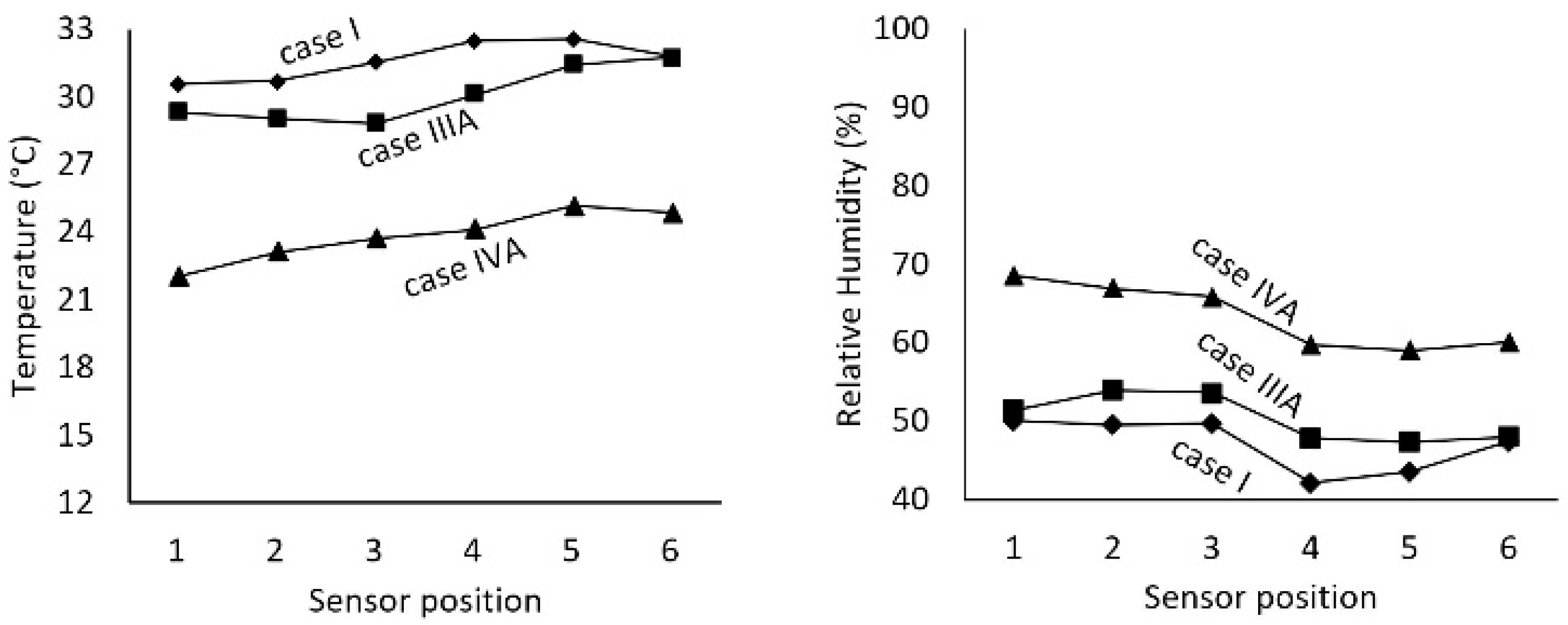
Temperature and RH recorded by sensors in an experimental greenhouse during the scenarios presented in Table 1 show that for the day, the temperature distribution in axes for case I, IIIA, and IVA (Figure 4) showed that in all cases, there was a tendency of temperature increase in the direction of the slope, thermal difference prevailing in consecutive axes between the 3, 4 and 5 with a value of 1 °C to 2 °C. In case I, the thermal difference was 1.96 °C between axis 1 and axis 5; for case IIIA, it was 2.92 °C between axis 3 and axis 6, and in the case, IVA was 3.14 °C between axis 1 and 5. The RH distribution (Figure 3) shows that in case I, the RH difference was 7.93% between axis 1 and axis 4; for case IIIA, it was 6.55% between axis 2 and axis 5, and in the case, IVA was 9.58% between axis 1 and axis 5. However, for cases I and IIIA, temperatures were above 30 °C, outside the maximum recommended threshold for tomato development [20,21].

The IVA case (December) presents a uniform temperature within the recommended range. Regarding RH, the IVA case increases 20% compared to the other cases, an increase caused by the appearance of cold fronts during the winter season.

3.3. Night-Time Period

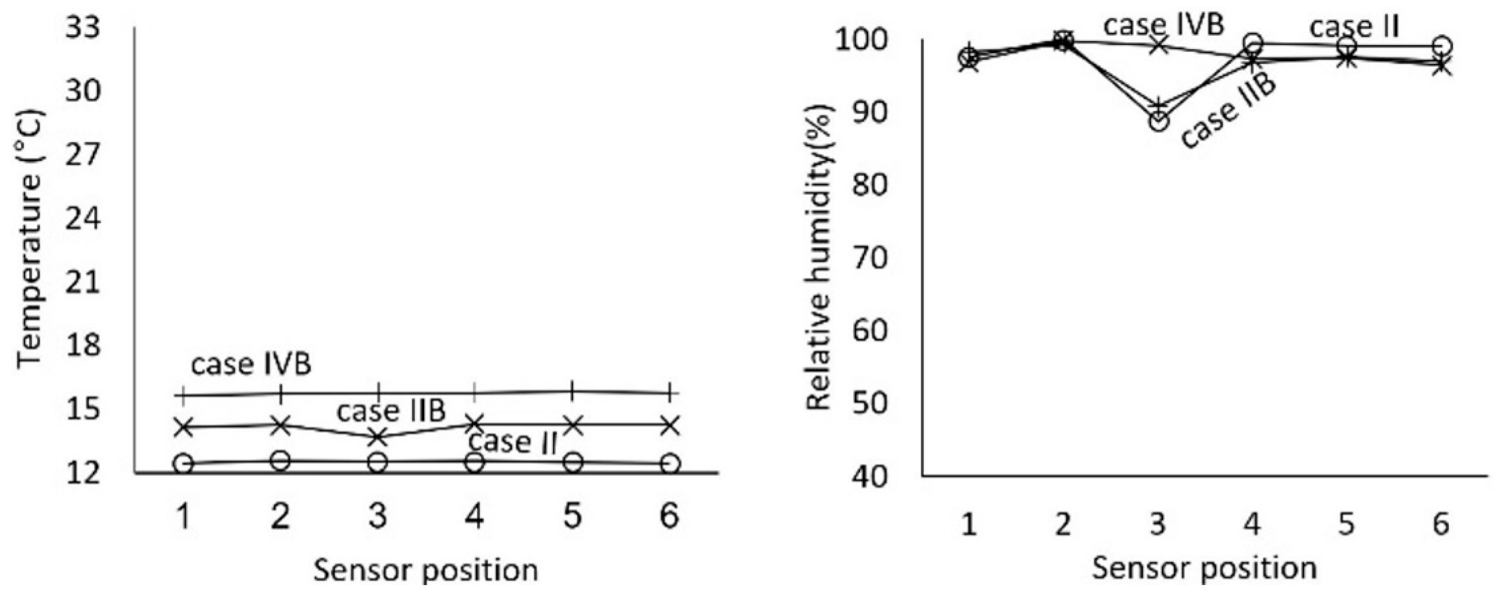
In case II, the thermal difference was 0.11 °C between axis 2 and 1. In case IIIB, it was 0.61 °C concerning axis 4, and in case IVB, the difference was 0.18 °C between axis 1 and 5. There is a higher temperature homogeneity than in the described cases of the diurnal interval (Figure 4). For RH (Figure 5), there is a tendency of an appreciable decrease in case II and IVB, of an appreciable decrease in axis 3, so in both cases, the moisture difference was lost from axis 2 to 3 with 11.25% 8.45%, respectively. For IIIB, a difference between axis 2 and axis 6 of 3.36% was obtained. However, the RH for all three cases exceeds the recommended maximum (50–70%), making it necessary to look for alternatives to reduce RH, avoid condensation inside the greenhouse and improve crop quality and yield.

The analysis by RH blocks in cases I, II, IIIA, IIIB, IVA, and IVB. There was an upward trend from block A to block C for cases I, IIIA, and IVA, with a difference between blocks of 3.3% for the case I, 3.79% for case IIIA, and 5.62% for IVA. While for cases II, IIIB and IVB, there was an increase from block A to B (Case I, 1.08 °C; Case IIIB, 0.99 °C; Case IVB, 1.41 °C) followed by a decrease in block C (Case I, 6.04%; Case IIIB, 0.92%; Case IVB, 4.02%).

Regarding the analysis by temperature blocks in case I, the most significant thermal difference was from block A to C (0.05 °C); in case II, it was from block A to B (0.15 °C); for case IIIA, it was from B to C (0.63 °C); in case of IIIB it was from A to C (0.37 °C); in case of IVA, it was from A to B (0.013 °C), and for case IVB it was from A to C (0.04).

3.4. Orthogonal Contrasts in the Slope Direction for Temperature and Relative Humidity

Orthogonal contrasts were performed to determine the effect of slope on temperature and RH, utilizing a statistical analysis grouping axes. If the contrasts are not orthogonal (p < 0.05), it implies covariance between them and is related to a certain degree. The results of the orthogonal contrasts are shown in

Table 5. Significance of orthogonal contrasts of temperature values.

Axis Grouping Contrast	1–2–3/4–5–6 (1)	1–2/5–6 (2)	1/6 (3)
Case I	0.0824	0.1076	0.3704
Case II	0.7833	0.6896	0.9441
Case IIIA	0.0067(p < 0.05)	0.007 (p < 0.05)	0.045 (p < 0.05)
Case IIIB	0.2476	0.7794	0.7708
Case IVA	0.0007 (p < 0.05)	0.0003 (p < 0.05)	0.0021 (p < 0.05)
Case IVB	0.2864	0.1777	0.3585

for temperature, which reflects that the IIIA and IVA cases obtained a significance greater than 0.05, so that for the IIIA case, contrast 1 (grouping axes 1, 2, and 3, and comparing them with axes 4, 5 and 6) obtained the most significant difference between groups, followed by contrast 2 (grouping axes 1, 2 and comparing them with axes 5 and 6) and finally contrast 3 (comparing axis 1 with axis 6). A higher significance value was obtained for the IVA case than in contrast 2, followed by contrast 1 and 3.

For RH,

Table 6. Significance of orthogonal contrasts of RH values.

Axis Grouping Contrast	1–2–3/4–5–6 (1)	1–2/5–6 (2)	1/6 (3)
Case I	0.1395	0.3141	0.694
Case II	0.2859	0.9424	0.8291
Case IIIA	0.1199	0.2156	0.5903
Case IIIB	0.0890	0.1552	0.7830
Case IVA	0.04 (p < 0.05)	0.0576	0.1672
CasoeIVB	0.5855	0.4823	0.6848

shows covariance in the case IVA in contrast 1, but not in contrast 2 and 3.

According to the orthogonal analysis between axes, it is observed that most of the cases present independence between the mean temperature values of the groupings. The cases that are not orthogonal present a higher covariance between a more significant number of grouped axes, as in contrast 1, and not for individually related axes, as in contrast 3. This tendency is also reflected in the temperature and RH distribution results, where there is a more significant temperature difference between axes 3, 4, and 5 during the day, especially in the daytime interval.

Likewise, there are more significant differences in the slope direction for both variables, not in the cross-section. There is a tendency for the temperature to rise as the altitude increases due to differences in densities and difference in altitude between axes and, in turn, a decrease in RH. In blocks, there is a slight upward trend in relative humidity in the daytime interval and a drop in block C in the night-time interval. In the case of temperature for both intervals, spatial uniformity is observed.

According to Lopez [22], the most significant differences in a flat greenhouse were 2.3 °C temperature and 5.3% relative humidity. The most significant differences were 3.14 °C and 11.25% between greenhouse extremes concerning the results obtained.

3.5. Behavior of Temperature and RH in the Days of Study in Relation to the Needs of the Crop

According to Tesi [23], the optimal intervals of RH are between 65% and 70% for pepper and between 55% and 60% for tomato. In the case of pepper, the suggested temperature range is between 22 °C to 28 °C during the day, and 16 °C to 18 °C at night. For tomatoes, it is between 22 °C to 26 °C during the day and between 13 °C to 16 °C during the night.

The temperature and RH distribution on October 6 and 23, November 7, and December 6 are shown in

Table 7. Temperature and RH recorded inside the greenhouse during the case studies.

Axis	Date	Day Time Period		Night-Time Period
		Tmax (°C)	RH (%)	Tmin (°C)	RH (%)
	6 October	31.04	45.60	14.04	97.42
1	23 October	30.81	46.24	13.08	96.13
	7 November	31.59	44.59	11.71	97.73
	6 December	22.06	69.01	14.94	98.27
	6 October	30.63	48.40	14.16	99.87
2	23 October	31.22	44.68	13.65	98.25
	7 November	33.01	39.18	12.18	100.00
	6 December	23.11	67.46	15.04	99.28
	6 October	30.24	48.71	14.16	98.78
3	23 October	31.84	40.16	13.89	96.15
	7 November	33.89	39.44	12.23	88.75
	6 December	23.75	66.14	15.09	90.86
	6 October	31.74	48.82	14.24	97.22
4	23 October	33.19	40.62	13.95	94.34
	7 November	35.40	31.20	12.22	99.94
	6 December	24.13	59.64	15.06	96.72
	6 October	33.26	41.92	14.23	97.49
5	23 October	33.39	39.71	13.87	95.10
	7 November	36.29	32.13	12.16	99.22
	6 December	25.17	59.37	15.10	97.64
	6 October	33.48	43.07	14.19	96.47
	23 October	32.77	43.07	13.88	94.34
6	7 November	37.44	32.59	12.12	99.40
	6 December	24.89	60.39	15.00	96.89

. During the day, the crops were not inside the optimum temperature range for approximately four hours, which could cause a higher incidence of pests and a decrease in crop yield. In the night period, the temperature conditions remained in the optimum range for the tomato. However, the RH remained in the optimum range for two hours before noon and between one and two hours in the afternoon. On December 6, the RH was outside the optimal range for the tomato, and at night the humidity increased to values above the maximum recommended for both crops, derived from the temperature drop.

According to the distribution of temperature and RH over the days analysed, it was observed that the times out of range are very high, and these affect crop yields, with the direct consequence of a decrease in the profitability of agricultural activity.

According to Leal and Costa [5], essential processes such as photosynthesis, respiration, and other plant processes depend on temperature, affecting plant growth and reproduction.

During high temperatures, the cells collapse due to the drought they suffer, so the stomata close automatically, limiting the loss of more water. By closing the stomata, CO₂ capture is reduced, causing a limitation of the photosynthesis process. Before a high temperature occurs, the plant stops its vegetative development. At low temperatures, proteins in plant cells precipitate and dehydrate.

In the case of RH, vapor pressure differences between leaf and air can increase evaporation losses, leading to wilting. Lack of humidity decreases pressure differences, and transpiration is intense. Low RH associated with high temperatures can cause leaf tip burn, and high RH stimulates the development of most germs and pathogenic organisms.

These aspects justify the need to generate tools that allow the correct design of protected environments according to the climate and define if it is necessary to resort to mechanical systems to correct the deficiencies that cannot be controlled utilizing the design with natural systems [24,25,26,27,28].

The presence of slopes in the soil influences the airflow; these conditions generate a loss of wind speed once the air enters the greenhouse causing it to be directed towards the roof windows in the opposite direction to the slope, with areas of low speed in the leeward side, as reported by Taloub et al. [29]; this effect is due to that during the day inside the greenhouse, there is a difference in temperature between the windward and leeward areas.

The behaviour of the greenhouse shows a temperature gain (areas with higher altitudes) for each of the scenarios studied during the day (12:30), where the air inside the greenhouse is heated by solar radiation, as demonstrated by [30]. This temperature increase is typical of structures on flat surfaces, where the thermal gradient is a function of the prevailing wind direction [31]. For this reason, it is necessary to study the thermal homogeneity of the greenhouses to reduce the effects caused when the maximum temperatures are higher than those recommended [32,33,34]. During the night (04:45), the thermal difference in the greenhouse was lower, given that the environmental heterogeneity depends on the level of solar radiation; these results are consistent with those reported by [31,34,35].

4. Future Analysis

One way to simulate the environment of a greenhouse to predict its thermal behaviour under natural ventilation conditions is by using the Computational Dynamic Fluid Computing (CFD) tool. Using computational models has allowed us to characterize and modify the variables that analytically affect greenhouse production [14]. In recent years, computational models have been used to simulate the thermal difference in different types of greenhouses [15,25,36,37], evaluating the effect of orientation [38], roofing material [20], airflow obstruction by vegetation, anti-insect proof mesh, and greenhouse length [26,38,39], looking for the increase in the renewal rate of air inside the greenhouse [27,28] and environmental comfort for the present crop.

5. Conclusions

The environmental analysis in the experimental greenhouse showed that there was not a stable stratification of the temperature, and RH in the direction of the slope was not found during the analysis period. The highest thermal difference within the greenhouse was presented in 3.14 °C in the slope direction and 0.63 °C in the cross-section direction. In the case of higher RH, it is 11.25% in the slope direction and 6.04% in the direction of the presented cross-section. Using the Tukey method and orthogonal contrasts, it was possible to demonstrate that 60.0% slope has no inference on the thermal difference in the greenhouse. For this reason, it is established that greenhouses on hillsides have a distribution very similar to that of greenhouses on a flat terrain. The design, height, length, and management are factors to be considered for the environmental comfort of the crops.

Most of the days analysed during the day were three consecutive hours outside the optimum temperature range for chili and tomato. In addition, during the entire night interval, they were outside the optimum RH for both crops, which could cause damage to the development and growth of the crops and increase the probability of growth of some pathogens. For this reason, it is established that greenhouses on hillsides have a distribution very similar to greenhouses on flat terrain, where the thermal gradient is a function of the prevailing wind direction. Therefore, it is necessary to study the thermal homogeneity of greenhouses to reduce the effects caused when maximum temperatures are higher than recommended, in order to seek future strategies to improve the design, height, length, and management, factors to be taken into account for the environmental comfort of the crops.

References

- Flores, J. Estudio Del Clima en Los Principales Modelos de Invernaderos en México (Malla Sombra, Multitunel y Baticenital), Mediante la Técnica Del CFD (Computational Fluid Dynamics). Ph.D. Thesis, University of Almería, Almería, Spain, 2010. [Google Scholar]
- McCartney, L.; Orsat, V.; Lefsrud, M.G. An experimental study of the cooling performance and airflow patterns in a model Natural Ventilation Augmented Cooling (NVAC) greenhouse. Biosyst. Eng. 2018, 174, 173–189. [Google Scholar] [CrossRef]
- Akrami, M.; Javadi, A.A.; Hassanein, M.J.; Farmani, R.; Dibaj, M.; Tabor, G.R.; Negm, A. Study of the effects of vent configuration on mono-span greenhouse ventilation using computational fluid dynamics. Sustainability 2020, 12, 986. [Google Scholar] [CrossRef] [Green Version]
- Rico-García, E.; Soto-Zarazua, G.M.; Alatorre-Jacome, O.; De La Torre-Gea, G.A.; Gomez-Melendez, D.G. Aerodynamic study of greenhouses using computational fluid dynamics. Int. J. Phys. Sci. 2011, 6, 6541–6547. [Google Scholar] [CrossRef]
- Leal, P.M.; Costa, E. Apostilla de Ingeniería de Confort en Cultivos Protegidos, 1st ed.; University of Campinas: São Paulo, Brasil, 2011. [Google Scholar]
- Villagran, E.; Leon, R.; Rodriguez, A.; Jaramillo, J. 3D numerical analysis of the natural ventilation behavior in a Colombian greenhouse established in warm climate conditions. Sustainability 2020, 12, 8101. [Google Scholar] [CrossRef]
- Bournet, P.E.; Boulard, T. Effect of ventilator configuration on the distributed climate of greenhouses: A review of experimental and CFD studies. Comput. Electron. Agric. 2010, 74, 195–217. [Google Scholar] [CrossRef]
- Aguilar-Rodríguez, C.E.; Flores-Velázquez, J.; Rojano, F.; Flores-Magdaleno, H.; Panta, E.R. Simulation of Water Vapor and Near Infrared Radiation to Predict Vapor Pressure Deficit in a Greenhouse Using CFD. Processes 2021, 9, 1587. [Google Scholar] [CrossRef]
- Soussi, M.; Chaibi, M.T.; Buchholz, M.; Saghrouni, Z. Comprehensive Review on Climate Control and Cooling Systems in Greenhouses under Hot and Arid Conditions. Agronomy 2022, 12, 626. [Google Scholar] [CrossRef]
- Sedat, B.; Adil, A. Effect of greenhouse cooling methods on the growth and yield of tomato in a Mediterranean climate. Int. J. Hortic. Agric. Food Sci. (IJHAF) 2018, 2, 199–207. [Google Scholar]
- Adams, S.R.; Cockshull, K.E.; Cave, C.R.J. Effects of temperature on the growth and development of tomato fruits. Ann. Bot. 2001, 88, 869–877. [Google Scholar] [CrossRef]
- Morales, D.; Rodriguez, P.; Dell’Amico, J.; Nicolas, J.; Torrecillas, A.; Sanchez-Blanco, M.J. High temperature preconditioning and thermal shock imposition affects water relations, gas exchange and root hydraulic conductivity in Tomato. Biol. Plant. 2003, 47, 6–12. [Google Scholar] [CrossRef]
- Peet, M.; Sato, S.; Clemente, C.; Pressman, E. Heat stress increases sensitivity of pollen, fruit and seed production in tomatoes (Lycopersicon esculentum Mill.) to non-optimal vapor pressure deficits. Acta Hortic. 2003, 618, 209–215. [Google Scholar] [CrossRef]
- Liu, X.; Li, H.; Li, Y.; Yue, X.; Tian, S.; Li, T. Effect of internal surface structure of the north wall on Chinese solar greenhouse thermal microclimate based on computational fluid dynamics. PLoS ONE 2020, 15, e0231316. [Google Scholar] [CrossRef] [PubMed] [Green Version]
- Bartzanas, T.; Boulard, T.; Kittas, C. Numerical simulation of the airflow and temperature distribution in a tunnel greenhouse equipped with insect-proof screen in the openings. Comput. Electron. Agric. 2002, 34, 207–221. [Google Scholar] [CrossRef]
- Benni, S.; Tassinari, P.; Bonora, F.; Barbaresi, A.; Torreggiani, D. Efficacy of greenhouse natural ventilation: Environmental monitoring and CFD simulations of a study case. Energy Build. 2016, 125, 276–286. [Google Scholar] [CrossRef]
- Reynafarje, X.; Villagrán, E.A.; Bojacá, C.R.; Gil, R.; Schrevens, E. Simulation and validation of the airflow inside a naturally ventilated greenhouse designed for tropical conditions. Acta Hortic. 2020, 1271, 55–62. [Google Scholar] [CrossRef]
- Villagrán, E.A.; Romero, E.J.B.; Bojacá, C.R. Transient CFD analysis of the natural ventilation of three types of greenhouses used for agricultural production in a tropical mountain climate. Biosyst. Eng. 2019, 188, 288–304. [Google Scholar] [CrossRef]
- Molina-Aiz, F.D.; Valera, D.L.; López, A. Airflow at the openings of a naturally ventilated Almería-type greenhouse with insect-proof screens. Acta Hortic. 2011, 893, 545–552. [Google Scholar] [CrossRef]
- Villagrán, E.; Bojacá, C.; Akrami, M. Contribution to the Sustainability of Agricultural Production in Greenhouses Built on Slope Soils: A Numerical Study of the Microclimatic Behavior of a Typical Colombian Structure. Sustainability 2021, 13, 4748. [Google Scholar] [CrossRef]
- Kobayashi, K.; Salam, M.U. Comparing Simulated and Measured Values Using Mean Squared Deviation and its Components. Agron. J. 2000, 92, 345. [Google Scholar] [CrossRef]
- Lopez, A. Validación de un Modelo Matemático Para Predecir Las Condiciones Climáticas Interna en un Invernadero Localizado en la Zona Norte de Cartago, Costa Rica. Bachelor Thesis, Universidad de Costa Rica, San Jose de Costa Rica, Costa Rica, 2012. [Google Scholar]
- Tesi, R. Medios de Protección Para la Horto Florofruticultura y el Viverismo, 3rd ed.; Mundiprensa: Madrid, Spain, 2001. [Google Scholar]
- Subin, M.C.; Lourence, J.S.; Karthikeyan, R.; Periasamy, C. Analysis of materials used for Greenhouse roof covering-structure using CFD. IOP Conf. Ser. Mater. Sci. Eng. 2018, 334, 012068. [Google Scholar] [CrossRef] [Green Version]
- Aguilar-Rodríguez, C.E.; Flores-Velázquez, J.; Rojano, F.; Ojeda-Bustamante, W.; Iñiguez-Covarrubias, M. Tomato (Solanum lycopersicum L.) crop cycle estimation in greenhouse, based on degree day heat (GDC) simulated in CFD. Tecnol. Cienc. Agua 2020, 11, 27–57. [Google Scholar] [CrossRef]
- Mesmoudi, K.; Meguallati, K.; Bournet, P.E. Effect of the greenhouse design on the thermal behavior and microclimate distribution in greenhouses installed under semi-arid climate. Heat Transfer–Asian Res. 2017, 46, 1294–1311. [Google Scholar] [CrossRef]
- Chu, C.R.; Lan, T.W.; Tasi, R.K.; Wu, T.R.; Yang, C.K. Wind-driven natural ventilation of greenhouses with vegetation. Biosyst. Eng. 2017, 164, 221–234. [Google Scholar] [CrossRef]
- Cemek, B.; Atiş, A.; Küçüktopçu, E. Evaluation of temperature distribution in different greenhouse models using computational fluid dynamics (CFD). Anadolu J. Agric. Sci. 2017, 32, 54. [Google Scholar] [CrossRef] [Green Version]
- Taloub, D.; Bouras, A.; Driss, Z. Effect of the Soil Inclination on Natural Convection in Half-Elliptical Greenhouses. J. Eng. Res. Afr. 2020, 50, 70–78. [Google Scholar] [CrossRef]
- Villagran, E.; Bojacá, C. Three-dimensional numerical simulation of the thermal and aerodynamic behavior of a roof structure built on a slope and used for horticultural production. Comun. Sci. 2021, 12, e3593. [Google Scholar]
- Villagran, E.; Bojacá, C. Analysis of the microclimatic behavior of a greenhouse used to produce carnation (Dianthus caryophyllus L.). Ornam. Hortic. 2020, 26, 109–204. [Google Scholar] [CrossRef]
- Ma, D.; Carpenter, N.; Maki, H.; Rehman, T.U.; Tuinstra, M.R.; Jin, J. Greenhouse environment modeling and simulation for microclimate control. Comput. Electron. Agric. 2019, 162, 134–142. [Google Scholar] [CrossRef]
- Saberian, A.; Sajadiye, S.M. The effect of dynamic solar heat load on the greenhouse microclimate using CFD simulation. Renew. Energy 2019, 138, 722–737. [Google Scholar] [CrossRef]
- Villagran, E.; Bojacá, C. Experimental evaluation of the thermal and hygrometric behavior of a Colombian greenhouse used for the production of roses (Rosa spp.). Ornam. Hortic. 2020, 26, 205–219. [Google Scholar] [CrossRef]
- Bojacá, C.R.; Gil, R.; Gómez, S.; Cooman, A.; Schrevens, E. Analysis of greenhouse air temperature distribution using geostatistical methods. Trans. ASABE 2009, 52, 957–968. [Google Scholar] [CrossRef]
- Villagrán, E.A.; Bojacá, C.R. CFD simulation of the increase of the roof ventilation area in a traditional Colombian greenhouse: Effect on air flow patterns and thermal behavior. Int. J. Heat Technol. 2019, 37, 881–892. [Google Scholar]
- Akrami, M.; Mutlum, C.D.; Javadi, A.A.; Salah, A.H.; Fath, H.; Dibaj, M.; Farmani, R.; Mohammed, R.H.; Negm, A. Analysis of inlet configurations on the microclimate conditions of a novel standalone agricultural greenhouse for Egypt using computational fluid dynamics. Sustainability 2021, 13, 1446. [Google Scholar] [CrossRef]
- Kuroyanagi, T. Investigating air leakage and wind pressure coefficients of single-span plastic greenhouses using computational fluid dynamics. Biosyst. Eng. 2017, 163, 15–27. [Google Scholar] [CrossRef]
- Jiao, W.; Liu, Q.; Gao, L.; Liu, K.; Shi, R.; Ta, N. Computational Fluid Dynamics-Based Simulation of Crop Canopy Temperature and Humidity in Double-Film Solar Greenhouse. J. Sens. 2020, 2020, 8874468. [Google Scholar] [CrossRef]
Figure 1.
(a) Dimensions of the experimental greenhouse and (b) Installation of the sensors.
Figure 2.
(a) Frequency analysis of the hours with higher temperatures in the daytime period. (b) Temperature values at 12:30 p.m. of the daytime period.
Figure 3.
(a) Frequency analysis of the hours with lower temperatures in the daytime period. (b) Temperature values at 04:45 am of the daytime period.
Figure 4.
Variation of temperature (°C) and RH (%) for daytime period.
Figure 5.
Variation of temperature (°C) and RH (%) for night-time period.