An Approach for Predicting the Effective Stress Field in Low-Permeability Reservoirs Based on Reservoir-Geomechanics Coupling

Abstract

Low-permeability reservoirs are important to the future growth of oil and gas reserves and production in China. Predicting the effective stress, σ_e, in reservoirs is vitally important due to its considerable impact on reservoir development through hydraulic fracturing. This paper presents methods for predicting the σ_e field in ultralow-permeability reservoirs through reservoir–geomechanics coupling, which involve the simulation and coupling of the tectonic stress σ and pore pressure P_p fields based on three-dimensional (3D) geological models. First, 3D geological models were constructed based on basic data for the oilfield where the reservoir of interest is located. Then, finite element and finite difference simulations were performed to construct the σ and P_p fields, respectively, in the reservoir. Different types of initial σ_e were coupled based on 3D geological models. Subsequently, a dynamic σ_e field in the reservoir was established based on oilfield production data in conjunction with the transformation, optimization, and coupling of specific grid property parameters obtained from different numerical methods. Finally, the proposed methods were tested on real-world data acquired from well area X in an oilfield in Shaanxi Province, China. The results show that the proposed methods can be used to establish the σ and P_p fields in a reservoir based on 3D geological models combined with different numerical methods, and subsequently predict the σ_e value in the reservoir.

1. Introduction

The rapid development of China’s national economy in recent years has led to an increasing dependence on oil resources. China’s current proven oil reserves are primarily located in complex reservoirs, including those with low permeabilities and special lithologies, those situated in complex fault blocks, and those bearing heavy crude oil [1,2]. China’s low-permeability oil and gas reservoirs, which are widely distributed in areas such as the Songliao, Ordos, and Sichuan Basins, and include large resource reserves, have broad prospects for exploration and development and are important to the future growth of energy reserves and production in the country [3,4].

Low-permeability reservoirs have low yields under natural conditions due to their poor physical properties [5,6,7] and often require large-scale hydraulic fracturing to reach a certain industrial production capacity. The formation and propagation of hydraulic fractures are controlled by the in situ stress. Predictions of the effective stress, σ_e, are crucial to efficient and rational reservoir development. For a low-permeability oilfield with a relatively homogenous reservoir medium, the direction along which hydraulic fractures extend (i.e., the direction of the maximum horizontal principal stress) is the direction of maximum seepage in its reservoirs.

Basic in situ stress data (primarily the tectonic stress σ and the pore pressure P_p) are essential to several aspects of oil and gas production, namely, reservoir engineering, exploration and drilling, and engineering scheme design [8]. An understanding of the in situ stress distribution pattern has important applications in areas such as the placement of development wells, the determination of the fracture distribution pattern, the control of the formation fracture pressure, the parametric design and control of directional wells, the estimation of the formation and impact of fractures in oil reservoir stimulation schemes, and sand control in oil wells [9,10]. The in situ stress also affects the direction of oil seepage and maximizing oil recovery [11].

From the aforementioned aspects, the in situ stress plays an important role in the low-permeability development. In detail, the effective stress controls the hydraulic fracturing and oil development, and is a concept that has been proposed for the stress that can deform porous media.

Sedimentary rock is a typical type porous media. Porous media are affected by external stress, i.e., external pressure or tectonic stress, and internal stress, i.e., internal pressure or pore pressure. Neither the external stress nor the internal stress can directly deform the porous media. They both deform the porous media through effective stress or skeleton stress. For the external and internal stress coupling, Terzaghi proposed a theory for the connection of the pore pressure (internal stress) and tectonic stress (external stress). According to Terzaghi’s σ_e theory, the in situ σ_e field during the development process is composed primarily of the σ withstood by the rock matrix and the pressure of the pore fluid (i.e., P_p). The relationship between injection and extraction continuously evolves as the development process advances, resulting in significant changes in the σ_e field. Predicting the changes in the σ_e field during the development process is pivotally important for subsequent steps involving the adjustment of the development scheme and the design of drilling, extraction, and fracturing schemes for new wells. Tectonic stress, or in situ stress, are usually simulated using FE methods and pore pressure are often simulated using the FD approach [6,7].

Some research has focused on directly solving reservoir–geomechanics coupling algorithms by developing coupling functions or models. Biot was the first to expand Terzaghi’s one-dimensional reservoir–stress coupling theory by proposing a three-dimensional (3D) in situ stress theoretical model [12,13]. Later, Geertsma introduced a theory of volume changes in porous rocks and discussed the effects of changes in the in situ stress on the elasticity of rocks and their pore volume [14,15,16]. Due to factors such as the popularization and application of hydraulic fracturing, in addition to the need to consider compaction-induced subsidence during the long-term extraction of oil and gas from reservoirs since the 1990s, researchers have considered changes in the in situ stress in the simulation of oil reservoirs and produced fruitful research results. A large number of reservoir–geomechanics coupling models have been successively developed. To solve the coupling models, the finite element (FE) method is more versatile compared to other methods (e.g., the finite difference (FD), discrete element, and boundary element methods).

The finite element method is the most common numerical simulation method for solving differential equations and partial differential equations. This method can effectively deal with different types of problems, and can also solve problems with highly complex set characteristics. Theoretically, the distribution of any physical quantity in multi-dimensional space can be described by the corresponding differential equation or partial differential equation, so the finite element method can effectively solve the distribution problem of any physical quantity in space. As a result of the continuous development of information technology, the finite element method has good applicability and accuracy for solving problems in various mechanical fields.

Initially, the finite element method was mainly used to solve the stress problems of structures in engineering mechanics. Later, the method was gradually extended to a series of other branches of physics, such as hydrodynamics, thermodynamics, and electromagnetism. The finite element method is also widely used in the field of geoscience, especially for the study of geomechanics. The finite element method can be used to study the local stress concentration phenomenon caused by the strength difference between the fault and the stratum. It can also be used to model geomechanical reservoirs via the finite element method, and for detailed analysis of the in situ stress, the influence of in situ stress on fluids, and the formation and deformation caused by in situ stress.

The finite element method provides a suitable solution and treatment means for reservoir discontinuity and anisotropy. The theoretical solution method is also relatively simple. It can be used to analyze the stress and strain mainly based on differential or partial differential equations. Moreover, this method can deal with highly heterogeneous strata and simulate complex boundary conditions and structural structures. Therefore, the magnitude, direction, and concentrated load distribution of in situ stress in the whole study area can be obtained using the finite element method. Therefore, the establishment of an in situ stress model based on the finite element method is widely used in in situ stress research.

Researchers have tried to establish many coupling models using the FE approach. These include the single- and dual-porosity reservoir–geomechanics coupling models developed by Teufel et al. [17,18] and Chen et al. [19]; the fully coupled FE models established by Cuisiat et al. [20]; the partially coupled FE models constructed by Settari et al. [21] and Tran et al. [22], which address the problem of poor convergence associated with full coupling; and the explicit integral coupling models proposed by Onaisi et al. [23,24] and Samier et al. [25] On this basis, Hatchell et al. [26], Herwanger et al. [27], and Onaisi et al. [28] developed four-dimensional dynamic in situ stress models that account for the time effect of production and injection processes. These models have been continually applied to new areas such as analyzing anisotropic formations and evaluating the sensitivity of permeability to stress. For the aforementioned models, researchers have only focused on building up the coupling approach through a single simulation approach, and have failed to combine different simulation approaches.

Another approach is to develop grid conversion-related algorithms to fulfill the requirements of reservoir–geomechanics coupling. This approach tries to combine different simulation methods and obtain the advantages of the different methods. The key parameters are then transferred from one model to another model to connect them. Park et al. developed a series of algorithms called PET2OSG to link the three-dimensional (3D) finite difference method (FDM)-based static model of Petrel with the 3D finite element method (FEM)-based fluid dynamic model of OpenGeoSys [29]. They also successfully employed these algorithms to simulate CO₂ storage in a saline aquifer [30]. FDM-based 3D grid models, especially the corner-point grid model, have been widely applied in oil and gas reservoirs to simulate the pressure, the oil saturation field, and well production [11,29,30,31,32,33,34]. Liu et al. developed a series of algorithms to simulate in situ stress using FEM based on a 3D corner-point grid model [11,31]. They also developed Petrel2ANSYS, which is an accessible software package for the simulation of crustal stress fields using grid conversion algorithms between FDM-based 3D grid models and FEM-based 3D grid models [32]. However, they only focused on the geomechanics aspects and simulated static in situ stress, and the dynamic models were neglected. Reservoir–geomechanics coupling algorithms were not employed, but the problem of different grid models was presented.

For fluid dynamic simulation, the finite volume and finite difference methods are often employed. The finite volume method is similar to the finite element method, and is mainly based on the law of physical conservation. This method is used to approximate the control domain of a discrete model through differential equations. However, since the finite volume method is mainly based on the numerical simulation method generated by computational fluid dynamics, almost all of the differential equations used in this method are Navier–Stokes equations [35]. The basic governing equations of the finite volume method mainly include three commonly used conservation equations: the mass conservation equation (continuity equation), the momentum conservation equation (motion equation), and the energy conservation equation [36]. After these equations are discretized, a point in the finite space is given to represent the sub-finite element volume by averaging in the finite control volume, which is usually the center point on the finite element surface or the center point of the volume. Subsequently, the control information contained in these points is only transmitted to the control points connected with them. This transmission mode is the biggest difference between this and the finite element method. In the finite element method, the transmission of control point information is controlled not only by adjacent elements, but also by other elements. Therefore, it transmits information with more points.

Due to the limitations of the finite volume method, the characterization and fitting are not accurate enough and are not suitable for mechanical transfer. However, because the matrix of this method is smaller, the solution speed is faster and the consumption of computing memory is less. At the same time, the finite volume method can also consider complex geometric model shapes. It can divide the model into multiple finite volume elements through a flexible mesh system, including hexahedral, tetrahedral, and polyhedral meshes. Based on the characteristics of the finite volume method, this calculation method is often used in the research of computational fluid dynamics to simulate the flow and heat transfer of fluid in engineering science [35]. The finite volume method is not a commonly used numerical simulation technology in geoscience, and some researchers have applied this method to the analysis of mixed interface movement in the process of salt and fresh water migration [37].

Compared with the finite element method, which uses differential equation approximation, the finite difference method characterizes the state at the element node by the approximate solution of the differential equation at that point. The finite difference method approximates the differential equation using the derivative of the governing equation. Through the finite difference method, a large solvable algebraic equation system is generated. By solving the equation system, the relevant information at each node is obtained [38]. The finite difference method can approximate the interpolation difference on a given set of points by the expansion of Taylor series and other methods. At the same time, the finite difference method requires a structured grid system for numerical simulation, such as a hexahedral grid [39]. In contrast to the finite element method, the nodes in the grid system are mainly the center points or corners of these grids, and the attributes of the grid reflect the average value of the grid attributes. In terms of this grid organization, the node distance of the grid can be changed, but in the case of dictation, it is difficult to apply this grid system, which has an uneven step size, due to the convergence of the solution [40]. The finite difference method has the advantages of fast calculation speed and reliable results. The finite difference method is widely used in discrete numerical simulation methods. However, this method cannot realize numerical simulation based on an unstructured grid and the spatial resolution of the model boundary is very inflexible, and is thus unable to achieve local refinement in boundary, fault, and other areas [40]. Therefore, the finite difference model cannot contain complex geometry.

In many cases of geoscience, the approximation of the domain boundary and interface with a rectangular grid element is accurate enough; for example, when simulating the flow of formation fluid, such as the groundwater flow in an aquifer [40]. Therefore, many studies use this numerical technique to simulate the migration of pollutants. In addition, this method is also suitable for seismic wave propagation models, such as references [35,38]. In addition to its application in earth science, the finite difference method is also generally applied to hydrodynamics applications, such as meteorological simulation.

The finite volume and finite difference methods are mainly applied to computational fluid dynamics, and are suitable for solving fluid saturation and pressure field problems. For the stress simulation, the finite element, discrete element, and boundary element methods are often used. Compared with the above three methods, because the boundary element method is mainly based on the integral form of the boundary differential equation, it cannot be effectively used in the absence of differential equations. Therefore, this method cannot effectively and accurately simulate the stress distribution for reservoirs having strong heterogeneity. The discrete element method is established based on the continuity characteristics of the object, but for the complex stress and strain elements of a reservoir, it is difficult to establish the corresponding stress model, which needs to be gradually improved. In contrast, the finite element method provides a better solution for reservoir discontinuity and anisotropy, and this method can deal with highly heterogeneous reservoirs and simulate complex boundary conditions. Through this method, the magnitude, direction, and concentrated load distribution of in situ stress can be obtained. Therefore, the establishment of in situ stress model based on the finite element method is widely used in in situ stress research.

Following the second approach, the existing 3D geological software packages, such as Petrel, developed by Schlumberger, can provide a detailed description of the underground reservoir information, but fail to simulate the in situ stress with the current FDM-based grid (the corner-point grid) models [33]. Moreover, the ECLIPSE software developed by Schlumberger can only perform reservoir pressure simulation using the corner-point grid [34]. FEM software such as ANSYS and ABAQUS are good toolkits for in situ stress modeling using 3D FEM-based grid models. They also fail to connect the FDM-based grid models due to different grid topology structures. There are certain gaps between FDM and FEM grid models. Although some studies have tried to connected the aforementioned grid models, they have only focused on the one-time conversion and linking of attributes. The application of the conversion and linking of attributes to reservoir–geomechanics coupling by employing different simulation methods and different software based on different grids has been rarely undertaken.

To fulfill the requirements of reservoir–geomechanics coupling by employing the aforementioned software based on different kinds of grid models, a series of algorithms have been designed. The designed algorithms can not only link the different grid models, but also transfer the vital information for different simulations’ requirements. In this study, firstly, an approach was designed to establish an initial σ_e field through the coupling of the reservoir and geomechanics fields based on the same 3D grid model, i.e., the corner-point based model. Secondly, on this basis, a multi-time coupling approach was designed to model a dynamic stress field through the coupling of the reservoir and geomechanics fields using the same 3D corner-point grid model. In this paper, the key algorithms, the transformations between the 3D corner-point (CP) and FE grid models used to simulate the stress field, the coupling of the grid parameters, and the transformations between the properties of the 3D CP and FE grids used to simulate the dynamic stress field are introduced in detail. The effectiveness of the methods developed in this study was tested on real-world data acquired from well area X in a certain oilfield. A 3D stress field model was constructed for the area, including the initial tectonic stress and pore pressure, along with the dynamic effective stress of different development times. In the final section of this paper, the conclusions are presented.

2. Establishment of an Initial σ_e Field through Reservoir–Geomechanics Coupling

According to Terzaghi’s σ_e theory, the in situ σ_e value consists of two parts: the σ that is primarily experienced by the rock matrix and the pressure of the fluid in the rock pores (i.e., P_p) (Equation (1)). Numerically, σ_e equals the difference between the σ experienced by the rock matrix and P_p. The σ_e value in a reservoir can be estimated by calculating σ and P_p. The P_p value in an oil reservoir can be simulated using the numerical FD simulation method, and the σ value can be determined in detail through FE simulations.

$$\overline{{\sigma }_e}=\overline{\sigma }-P_p$$

(1)

where $\overline{{\sigma }_e}$ is the effective stress field in the reservoir, $\overline{\sigma }$ is the tectonic stress field in the reservoir, and $P_p$ is the pore pressure field in the reservoir.

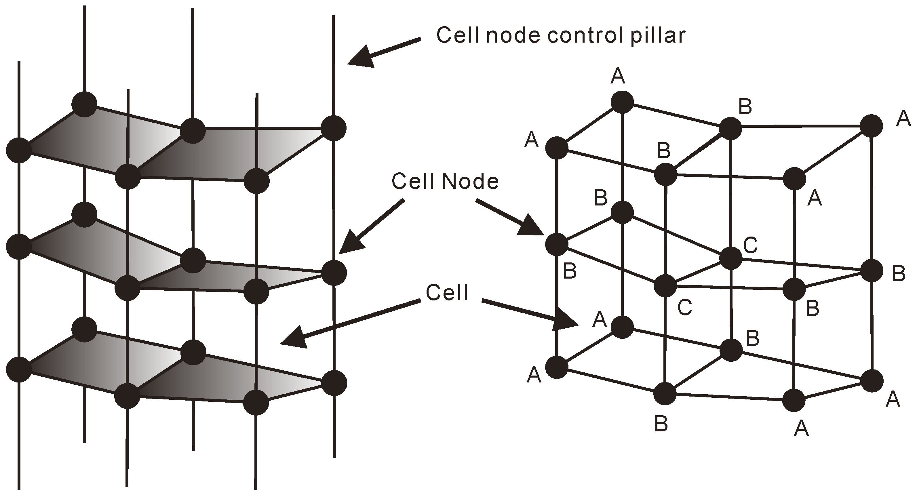
As a type of gridded model that describes spatial distributions, 3D geological models are effective at describing and characterizing the distribution patterns of the internal properties of geological bodies. Grid systems suitable for different numerical simulations and computations can be generated based on specific grid partitioning modes. As a common type of structured grid model, CP grid models are extensively used to simulate geological properties in three dimensions. The data organization mode and structure of CP grid models are highly compatible with the FD method.

To more flexibly capture the morphological characteristics of geological bodies, certain rules are set to govern the mode of indexing grid cells and nodes in 3D geological models based on CP grids and their topology. However, these rules have a certain impact on the transfer of properties (e.g., mechanical properties) in the FE method. Consequently, this type of grid system does not support numerical FE simulations. A 3D model based on a CP grid can be optimized into a grid model suitable for numerical FE simulations through the design of an algorithm that allows for transformations between CP and FE grids. In this way, FE simulations can be performed based on a CP-grid-based 3D model to depict the σ value. Therefore, one 3D geological model allows for both FD and FE simulations and is compatible with multiple software platforms. The simulations yield the P_p and σ fields, which are used to establish a σ_e field for the reservoir. For FD simulations, the models are compatible with the Schlumberger Petrel RE platform. For FE simulations, data analysis support is provided for common large-scale FE simulation software platforms (e.g., ANSYS and ABAQUS).

The procedure for establishing an initial 3D in situ σ_e field in the area of interest involves the following steps (Figure 1). There are three main processes: the data preparation process, the simulation process, and the coupling process.

The 3D modeling processes are the main data source. The models can be provided by other researchers, such as the geologists. First, a series of 3D geological property models are constructed for the area based on a CP grid in combination with basic oilfield data. These models are the essential data for the following analysis. In detail, the 3D property models mainly include two sets of models: (1) models required to simulate the initial σ value (i.e., a 3D Young’s modulus model, a 3D Poisson’s ratio model, a 3D rock density model, and an additional 3D rock cohesion model if the viscoelastic properties of the rock are considered); and (2) models used to establish the initial P_p field (i.e., a 3D porosity model, a 3D three-directional rock permeability model, a 3D oil saturation (OS) model, and models of other relevant properties (e.g., net-to-gross ratio (NGR)) used as the input for the numerical simulation of the oil reservoir.

For the simulation process, there are two steps. The first step: The data topology of the 3D Young’s, Poisson’s ratio, and rock density models based on corner-point grids, thereby enabling them to provide effective support for the numerical FE simulation method using grid conversion approaches integrated in in-house development software. Then, the FE method is employed to numerically simulate the 3D σ field in the area. The normal and shear stresses and the component of the principal stress in each direction are thus obtained. On this basis, a 3D initial σ field model for the area is constructed.

The second step: The FD method is used to establish an initial P_p model for the area based on models such as the 3D porosity and three-directional permeability models in conjunction with real-world oilfield production data. The grid models can directly support this simulation approach. Thus, grid conversion and modification do not need to operate. This completes the simulation process.

Finally, for the coupling process, Terzaghi’s σ_e theory is followed to construct a 3D σ_e model for the area, thereby characterizing the reservoir and geomechanics fields in a coupled manner. The initial σ field models are converted to support FE simulation. Here the models are converted back to corner-point-based models to support stress coupling.

Many shortcomings may exist due to data unreliability. The 3D models provided by other experts may not reflect the real distribution situation of the corresponding attributes, which may affect the results. For this work, we considered these models as being reliable and as the basic data source. We only focused on the target formation, and the upside and downside formations were considered to be impermeable to prove that the pore pressure is reliable. The oil only flows at the target reservoir.

The components of σ in different directions obtained during the simulation process can be combined with the distribution pattern of P_p to establish a fine 3D σ_e model for the area (Equation (2)) to support steps such as the adjustment of the development scheme for the oil and gas reservoir and the design of fracturing schemes. Alternatively, the mathematical means in the three directions (Equation (3)) can be used to describe the 3D stress model for the area in a homogenized manner.

$${\sigma }_{ei}={\sigma }_i-P_p,i=x,y,z$$

(2)

where ${\sigma }_{ei}$ represents the effective stresses in the reservoir in the x-, y-, and z-directions, respectively; ${\sigma }_i$ represents the tectonic stresses in the reservoir in the x-, y-, and z-directions, respectively; and $P_p$ is the pore pressure in the reservoir.

$$\{\begin{array}{l}\overline{{\sigma }_e}=\overline{\sigma }-P_p\\ \overline{\sigma }=\frac{1}{n}{\displaystyle \sum _{i=1}^n{\sigma }_i}\end{array} \mathrm{or} \overline{{\sigma }_e}=\frac{1}{n}{\displaystyle \sum _{i=1}^n{\sigma }_{ei}},i=x,y,z$$

(3)

where $\overline{{\sigma }_e}$ is the effective stress field in the reservoir; $\overline{\sigma }$ is the tectonic stress field in the reservoir; $P_p$ is the pore pressure in the reservoir; ${\sigma }_{ei}$ represents the effective stresses in the reservoir in the x-, y-, and z-directions, respectively; and ${\sigma }_i$ represents the tectonic stresses in the reservoir in the x-, y-, and z-directions, respectively.

3. Establishment of a Dynamic σ_e Field through Reservoir-Geomechanics Coupling

This process is similar to the initial effective stress modeling process. In general, the initial effective stress modeling process is considered as a one-time coupling for tectonic stress and pore pressure. The dynamic effective stress modeling process is considered as a multiple-time coupling for tectonic stress and pore pressure. For this process, several key attributes are needed to be transferred during the grid conversion time. The FE and FD methods can be used to establish a 3D σ_e model for the area of interest based on a CP grid model combined with Terzaghi’s σ_e theory. The initial σ_e field can no longer meet the urgent needs of development as this process continuously advances, and measures such as water injection are implemented. To characterize the in situ σ_e field in the area at different time points in more detail, a dynamic σ_e field is established for the area through dynamic coupling of the reservoir and geomechanics fields based on different time nodes of development. The main procedure for establishing a dynamic σ_e field through reservoir–geomechanics coupling involves the following steps (Figure 2). There are three processes included in this approach: the data preparation process, the simulation process, and the coupling process.

To start the simulations, the 3D models based on CP grid system are first imported. Then, the grid conversion and modification are performed to support FE simulations. Some other data required are also imported. Here the data preparation process is finished.

For the simulation process, first, the initially established 3D σ and P_p models are calculated using the aforementioned approach, which are the basic data for the following simulation. The simulated 3D σ field contains three-directional strain and volume strain properties, and the simulated P_p field reservoir pressure and oil saturation attributes. Here, judgements are used about whether the time steps are completed. If some time steps remain, the calculations are continued. Then, the coordinates are transferred using the FE simulation results, and the data and constraints of the initial 3D σ and P_p field models are then updated based on the current production conditions to calculate the characteristics of the σ field and P_p field in the subsequent time step. The boundary situations for the FE simulation are updated based on the results of the FD simulation results. The porosity and permeability models are updated using the FE simulation results.

For example, the distribution pattern of the σ field under the current production conditions can be determined through the correction of the grid at the boreholes for the Young’s modulus, Poisson’s ratio, and rock density, and the correction of the pressure boundary conditions using the P_p field calculation results. At the same time, the pore pressure field is also simulated using the FD method to obtain the pressure and oil saturation deviations. The boundary situations are updated using the σ field simulation results, and the three-directional strain and volume strain attributes. The porosity of the grid, which is essential in FD simulations, is updated based on the volume strain properties. Subsequently, the three-directional permeability of the grid model is updated based on the updated porosity. The FD simulation conditions are updated based on the OS and P_p properties in the previous time step. Then, a 3D σ and P_p field under the current conditions is simulated based on the updated property models. A new 3D σ and P_p model for the new time step for the area is thus established. For every time step, the processes are performed until all time steps are finished. In general, for every time step, there are new 3D σ and P_p models with different grid coordinates because of the deformation caused by the two stress couplings.

The final process is the coupling process. After the calculations for all the time steps are complete, the 3D σ and P_p fields are coupled to establish a final σ_e field model using Equations (1)–(3). A dynamic field stress field is thus constructed and characterized through the coupling of the reservoir and geomechanics fields with different time scales.

For the adjustment of the boundary conditions, each surface load and constraint can be set independently to adjust different conditions, including normal and abnormal compaction trends. Furthermore, the different loads do not have uniform values, but are set on each grid surface for the boundary cells. Considering the petrophysical/geomechanical properties with in-depth mechanical compaction domain and chemical compaction domain reservoirs, the only setting for this situation is the adjustment of the boundary load and constraints, and the internal rock mechanic parameter models are built with different values to reflect the difference. Moreover, when dealing with exhumed/uplifted basins, and the relevant depths are not the maximum burial depth, we can adjust the top load and bottom load for every boundary grid.

4. Key Techniques

4.1. Model Grid Transformation and Optimization

To establish an initial σ_e model for a reservoir, the σ_e value in each of the three directions must be determined, which can be achieved by establishing the initial σ field through FE simulations and the initial P_p field through FD simulations. The establishment of the initial stress field involves two numerical simulation methods, namely, the FD and FE methods. Numerical methods differ in terms of their grid partitioning and data organization modes. To unify the grid-based 3D geological property models, regular hexahedral grid elements are used as the basic cells based on the indexing mode of CP grids (Figure 3) [23,24]. Figure 3 shows the composition of a hexahedral CP grid. The locations of the grid nodes depend on their control columns. Each grid cell is composed of eight grid nodes. Nodes in this type of grid can be categorized into three types based on the indexing and storage modes: A, B, and C types (Figure 3). Type A nodes are constituents of individual grid cells; that is, they are not shared by different grid cells. Type B nodes are shared by two adjacent grid cells. Type C nodes are shared by four adjacent grid cells. According to the data organization mode for this type of grid, a type A node contains one grid node, a type B node contains two grid nodes with identical coordinates, and a type C node contains four grid nodes with identical coordinates. This type of grid indexing mode can effectively control the grid shape, thereby ensuring the accuracy of the 3D model.

Due to their different partitioning and indexing modes, hexahedral CP grid systems cannot be directly applied to the numerical FE simulation method. Based on lessons drawn from the grid transformation and optimization methods for complex models [11,32], a CP grid is transformed through its bottom-layer data, which enables the entire model to be calculated based on the numerical FE simulation method. This approach includes two main grid transformation steps, namely, CP-to-FE and FE-to-CP grid transformations.

The grid transformation techniques for complex models can be used to transform a CP grid model to an FE grid model while effectively recording the location information for the corresponding properties (Figure 4). Each cell of the FE grid transformed from the CP grid still contains eight grid nodes. However, this type of grid often transfers properties (e.g., mechanical properties) through the common nodes shared by adjacent cells. Therefore, the FE grid contains only one type of node. Based on the indexing and storage modes of the CP grid, the information at all the nodes is extracted, and all the duplicate nodes are removed. On this basis, a new indexing mode for the grid nodes is established. Then, the mapping relations between the grid nodes and the cells are reconstructed based on their original mapping relations. While the shape of the grid cells is preserved, the mapping relations between the FE grid nodes and the cells are established. Under this condition, all the cells of the grid model are correlated through common nodes, allowing for the transfer of properties (e.g., mechanical properties) and FE simulations.

In contrast to conventional methods, in terms of the FE-simulated grid properties, the three-directional strain and volume strain properties of the in situ stress in the 3D FE grid model, the shear and normal stresses, and the components of the principal stress in the three directions must be extracted during the FE-to-CP grid transformation process. The changes in the grid nodes are effectively recorded through the three-directional strain properties of the grid. During the FE-to-CP grid transformation process, the coordinate information for the grid nodes is updated to form a new CP grid system. The strain information results in changes in the node information for the CP grid model after the transformation process. However, the property information for the grid remains stored in the corresponding cells (Figure 5). In Figure 5, the grids before and after the FE simulations are shown in black and gray, respectively. The FE simulations may deform the grid cells. The data of the grid models describing σ and P_p are organically unified through the reconstruction of the indexing relationships between the grid nodes and cells, which is achieved through the reconstruction of the node indexes. The transformations between the CP and FE grids enable the initial σ_e field to be established through the coupling of the reservoir and geomechanics fields.

4.2. Coupling of the Property Parameters of the Dynamic Stress Field Grid

To effectively capture the dynamic changes in the stress field in a reservoir, the shape and internal properties of the cells of the 3D grid model describing the geological properties of the reservoir should vary with the external stress conditions at different time nodes or steps. The coordinates of the locations of the grid nodes obtained from the FE simulations can effectively record the changes in the shape of the grid cells.

During the simulation of a dynamic stress field, a one-way coupling method is applied in this study to the properties of the grid cells. Specifically, the corresponding stress and strain properties obtained from the FE simulations are used to update the cell properties of the 3D CP grid model (Touhidi-Baghini, 1998). Rocks are a type of porous medium. The deformation of a rock under external loading is mostly attributed to the changes in its pore spaces, while its matrix undergoes small deformations. Therefore, the porosity property of the cells of the grid model can be updated based on the volume strain data (Equation (4)). The three-directional rock permeability is another factor that significantly affects FD simulations. Based on the porosity–permeability relationship, the permeability property of the corresponding cells of the grid model is updated using the Carman–Kozeny equation (Equation (5)). As the calculation is based on the grid model for a low-permeability reservoir, the equation can be employed at the current scale. Some studies have discussed the deviation about this equation due to the variation in the porosity [41]. Moreover, other porosity–permeability equations can be employed instead of the current equation.

$${\varphi }_{new}^{\prime }=\varphi +{\epsilon }_v$$

(4)

$$k_{new}^{\prime }=k\cdot \frac{\left(1-{\varphi }^2\right){\varphi }_{new}^{\prime }{}^3}{\left(1-{\varphi }_{new}^{\prime }{}^2\right){\varphi }^3}$$

(5)

where ${\varphi }_{new}^{\prime }$ is the new porosity of the grid after the simulation (dimensionless), ϕ is the porosity of the grid before the simulation (dimensionless), ${\epsilon }_v$ is the volume strain of the grid cells (dimensionless), $k_{new}^{\prime }$ is the new permeability of the grid after the simulation (mD), and $k$ is the permeability of the grid before the simulation (mD).

5. Case Study

Well area X in a certain oilfield in Shaanxi Province, China, was selected for a case study. The area above the Change-6 oil reservoir in well area X consists of a typical landform commonly observed on the Loess Plateau, which is characterized by crisscrossing ravines and gullies interspersed with ridges and hills. The ground elevation generally ranges from 1350 to 1850 m, resulting in a large relative elevation. The Change-6 oil reservoir developed primarily in a delta-front subfacies environment. The delta-front sediments were deposited mainly in underwater distributary channels, underwater interdistributary bays, and underwater natural dike microfacies environments. The lithology of the reservoir is composed predominantly of fine-grained lithic feldspar sandstone. The pores in the reservoir rock, which mainly consist of small feldspar dissolution and intergranular pores with narrow throats, are primarily filled with hydromica, chlorite, ferrocalcite, and siliceous materials.

In general, the Chang-6 oil reservoir in well area X has poor physical properties, with porosity values ranging from 0.10 to 23.05%, an average porosity of approximately 3.29%, permeability values ranging from 0.010 to 40.879 mD, and an average permeability of 0.104 mD, suggesting that this reservoir is a typical ultralow-permeability reservoir. Lithologic in nature and driven by elastic dissolved gas, this reservoir is buried at a depth of 2650 m and contains oil, oil–water, and poor oil layers with average thicknesses of 2.2, 10.7, and 4.6 m, respectively. With an original formation pressure of 20 MPa and a pressure coefficient of 0.88, this oil reservoir is categorized as an abnormally low-pressure reservoir.

The reservoir rock in well area X has density values ranging from 1.44 to 2.73 g/cm³, and an average density of 2.55 g/cm³; Young’s modulus values ranging from 3.84 to 55.33 GPa, and an average Young’s modulus of 36.45 GPa; Poisson’s ratio values ranging from 0.29 to 0.46, and an average Poisson’s ratio of approximately 0.33; and a brittleness index ranging from 0.03 to 0.87, and an average brittleness index of 0.37. The crude oil contained in the reservoir has good properties. The formation crude oil has a viscosity of 1.46 mPa⋅s, a density of 0.752 g/cm³, and a gas–oil ratio of 77.8 m³/t. The formation water is of the CaCl₂, type with a total mineralization degree of 26.9 g/L. Toxic and harmful gases (e.g., H₂S) were not detected in the associated gas samples collected for analysis.

The exploration of the Chang-6 reservoir in well area X began in 2016. To date, 76 exploratory and appraisal wells and 23 test wells have been drilled into this reservoir. Of the test wells, 14 meet the commercial oil flow standard. On average, the test wells each have an oil yield of 9.1 m³/d and a water yield of 3.2 m³/d. The development of the oil reservoir in well area X started in 2017 when the drilling of a total of 23 development wells was completed. In 2018, 20 highly deviated wells (HDWs) with a production capacity of 25,000 t were planned. Another 38 HDWs with a production capacity of 36,000 t were planned the following year. To date, 51 HDWs have been drilled, with an average oil-layer thickness of 75.4 m encountered during the drilling process. Pilot runs of 28 of these 51 wells have been completed. During the pilot runs, these wells each yielded an average of 4.5 t of oil (containing 48.4% water) daily. Currently, these wells each produce 3.2 t of oil (containing 45.2% water) daily.

Using optimized variants of software programs designed by previous researchers [31,32,42,43], the method introduced in Section 2 was used to transform 3D CP-grid-based property models (e.g., 3D Young’s modulus, Poisson’s ratio, and brittleness index models) for the area. The transformed models were then solved through numerical FE simulations to establish a 3D grid model to describe the σ values in the area. This model was subsequently optimized to construct a CP-grid-based 3D σ model. Models such as 3D porosity, permeability, and OS models were directly solved through numerical FD simulations to construct a 3D P_p model for the area. Finally, based on Terzaghi’s σ_e theory, the 3D σ model and the 3D P_p model were organically coupled to construct a CP-grid-based initial σ_e field (Figure 6).

To validate the simulation results, 16 rock samples were extracted from four wells, and four rock core samples for each well, representing the x-direction, y-direction, z-direction, and 45-grade direction (the μ-direction). The tectonic stress values were measured with certain confining values as listed in

Table 1. The simulated and test tectonic stress values or the target area.

Well Name	Core Sample Direction	Confining Pressure	Kaiser Point (MPa)	Vertical Stress (MPa)	Maximum Horizontal Stress (MPa)	Minimum Horizontal Stress (MPa)	Simulated Vertical Stress (MPa)	Simulated Maximum Horizontal Stress (MPa)	Simulated Minimum Horizontal Stress (MPa)
Well 1	x	20	51.11	64.18	59.07	55.87	60.23	56.7	51.82
	y		50.98
	z		54.3
	μ		59.42
Well 2	x	20	53.71	63.38	58.61	53.64	59.24	56.33	49.81
	y		41.83
	z		49.01
	μ		58.62
Well 3	x	20	54.16	64.71	58.97	54.09	59.37	53.72	50.38
	y		57.31
	z		49.37
	μ		59.94
Well 4	x	25	60.74	64.97	59.99	55.66	60.13	55.42	51.71
	y		57.87
	z		56.41
	μ		65.72

. The simulated stress values were compared with the test values. The results show that simulated results are well fitted with the test values.

Based on the CP-grid-based initial σ_e field established through reservoir–geomechanics coupling in combination with real-world production data, the method introduced in Section 3 to establish a dynamic σ_e field was employed to derive stress field models for different production time points (for example, after five and 10 years) (Figure 7). The continuous advancement of the oilfield development process resulted in considerable changes in the P_p values in the area, which in turn significantly impacts the σ_e values in the reservoir. In the absence of reservoir stimulation measures (e.g., hydraulic fracturing), depletion development caused small changes to the σ values experienced by the reservoir rock, leading to minor changes in the σ_e values in the reservoir.

6. Conclusions

This paper presents methods for modeling the initial and dynamic σ_e fields through the coupling of the reservoir and geomechanics fields using 3D models based on corner-point grid models. The key techniques involved in the methods are described. In addition, the effectiveness of the methods was tested on real-world data acquired from well area X in a certain oilfield in Shaanxi Province, China. The conclusions of this study are summarized below:

• Based on the transformation and optimization algorithms of grid models, an approach for modeling the initial σ_e field in an area through the coupling of the reservoir and geomechanics fields was designed and implemented. In addition, 3D CP grid models were modified to support the simulation using the FE and FD methods in combination with improved grid transformation and optimization algorithms to construct 3D σ and P_p fields for the area. Then, a 3D σ_e model for the area was established through reservoir–geomechanics coupling using these models.
• An approach was designed to model the dynamic stress field through the coupling of the reservoir and geomechanics fields through one-way coupling of the grid properties in combination with grid transformation and optimization algorithms considering the time scale. The properties of the 3D grid models established to describe the σ and P_p fields in the area were coupled and updated using the FE and FD methods, respectively, to construct 3D σ and P_p fields for different time points, which were subsequently coupled to establish 3D σ_e models for the area for different time points. Furthermore, an in-house software platform was developed to conduct the reservoir–geomechanics coupling.
• Based on 3D geological model data and relevant production data for well area X in a certain oilfield in Shaanxi Province, China, the proposed methods for modeling the initial and dynamic stress fields through the coupling of the reservoir and stress fields were employed to construct a 3D initial σ_e field and 3D σ_e models for different production time points for well area X. The results were used to examine the feasibility of the proposed methods.