Article

Hybridized Particle Swarm—Gravitational Search Algorithm for Process Optimization

1
Department of Computer Science and Engineering, Koneru Lakshmaiah Education Foundation, Vaddeswaram 522 302, India
2
Department of Computer Science and Engineering, Vel Tech Multi Tech Dr. Rangarajan Dr. Sakunthala Engineering College, Chennai 600 062, India
3
Department of Machining, Assembly and Engineering Metrology, Faculty of Mechanical Engineering, VSB-Technical University of Ostrava, 17. Listopadu 2172/15, 708 00 Ostrava, Czech Republic
4
Department of Computer Science and Engineering, Sona College of Technology, Salem 636 005, India
5
Department of Aerospace Engineering and Applied Mechanics, Indian Institute of Engineering Science and Technology, Shibpur 711 103, India
6
Department of Mechanical Engineering, Vel Tech Rangarajan Dr. Sagunthala R&D Institute of Science and Technology, Avadi 600 062, India
*
Authors to whom correspondence should be addressed.
Processes 2022, 10(3), 616; https://doi.org/10.3390/pr10030616
Submission received: 26 January 2022 / Revised: 17 March 2022 / Accepted: 19 March 2022 / Published: 21 March 2022

Abstract

:
The optimization of industrial processes is a critical task for leveraging profitability and sustainability. To ensure the selection of optimum process parameter levels in any industrial process, numerous metaheuristic algorithms have been proposed so far. However, many algorithms are either computationally too expensive or become trapped in the pit of local optima. To counter these challenges, in this paper, a hybrid metaheuristic called PSO-GSA is employed that works by combining the iterative improvement capability of particle swarm optimization (PSO) and gravitational search algorithm (GSA). A binary PSO is also fused with GSA to develop a BPSO-GSA algorithm. Both the hybrid algorithms i.e., PSO-GSA and BPSO-GSA, are compared against traditional algorithms, such as tabu search (TS), genetic algorithm (GA), differential evolution (DE), GSA and PSO algorithms. Moreover, another popular hybrid algorithm DE-GA is also used for comparison. Since earlier works have already studied the performance of these algorithms on mathematical benchmark functions, in this paper, two real-world-applicable independent case studies on biodiesel production are considered. Based on the extensive comparisons, significantly better solutions are observed in the PSO-GSA algorithm as compared to the traditional algorithms. The outcomes of this work will be beneficial to similar studies that rely on polynomial models.

1. Introduction

In the last few decades, many researchers have proposed numerous optimization techniques to find the best values among the sets of alternatives. Many researchers have used metaheuristic techniques to find the optimal values. Metaheuristic techniques are mostly optimization techniques inspired by nature and natural phenomena. Some examples of nature-inspired metaheuristic techniques are the genetic algorithm (GA) [1], particle swarm optimization (PSO) [2], artificial bee colony (ABC) [3], bat algorithm (BA) [4], gravitational search algorithm (GSA) [5], ant colony optimization (ACO) [6], differential evolution (DE) [7], ant lion optimization (ALO) [8], multi-verse optimization (MVO) [9], salp swarm algorithm (SSA) [10], grey wolf optimization (GWO) [11], dragonfly algorithm (DA) [12], whale optimization algorithm (WOA) [13], firefly algorithm (FA) [14], etc. All population-based metaheuristic optimization algorithms have two main parts—exploration and exploitation. Some optimization techniques are very good at exploration, and some are very good at exploitation. So, an optimizer with good exploration and bad exploitation is often combined with an optimizer with bad exploration and good exploitation to form a hybrid optimizer. Thus, the hybrid optimizers are very good at both exploration and exploitation. Some hybrid metaheuristic techniques are GA-PSO [15], WOA-SA [16], CS-DE [17], PSO-CS [18], PSO-GSA [19], etc.
In this paper, as a case study, the industrial use case of biodiesel production is analyzed. The rationale behind this is that alternate fuel demand is at an all-time high. Biodiesel in this regard is a promising sector. However, to ensure the rapid adoption of biodiesel, it is necessary to improve the existing yields and bring down the associated costs. Though the biodiesel generation process is fairly standardized, the process parameters involved have a significant impact on the overall effectiveness of the process. Thus, as a test case for the hybrid algorithms, the biodiesel industry is focused on in this paper. Researchers have mostly relied on multi-criteria decision making (MCDM) methods for optimization in this industry. However, MCDMs methods need a decision matrix, that is made up of the responses to be optimized. Thus, the MCDM method is limited by the provided decision matrix that are often recorded on discrete points. MCDMs work by locating the best solution (in terms of some weighted measure of multiple conflicting alternatives) among the supplied discrete points. By level averaging of the process parameters, the best process parameter levels can also be identified. On the other hand, since metaheuristics directly use objective functions that can perform continuous search in the search space, they are likely to return better optimal values than MCDMs.
A few works on metaheuristics-based optimization of biodiesel production process are seen in the literature. Betiku et al. [20] performed the optimization of process parameters of biodiesel production from shea tree nut butter using the GA, neural network and response surface methodology. The objective of their work is to maximize the biodiesel yield. Garg and Jain [21] performed optimization of process parameters of biodiesel production from algal oil using RSM and ANN. They considered reaction time, catalyst amount, and methanol/oil ratio as process parameters and yield as a response parameter. Miraculas et al. [22] examined process parameter optimization for biodiesel production from mixed feedstock using an empirical model. Patil and Deng [23] optimized biodiesel production from edible and non-edible vegetable oils. Outili et al. [24] optimized biodiesel production from waste cooking oil. They considered temperature, catalyst amount, and methanol/oil ratio as independent variables and conversion, and energy and green chemistry balance as dependent variables to design the regression model. It is observed that for expressing responses as functions of process parameters, mostly RSM (polynomial regression) is used in the literature [20,22,23,24,25,26]. However, the use of neural networks has also gained traction in the last decade [21,27,28].
In this paper, two hybrid metaheuristic algorithms are developed by combining the iterative improvement capabilities of PSO and GSA. The hybrid algorithms are called PSO-GSA and BPSO-GSA and are compared against several traditional algorithms to demonstrate their efficacy. The BPSO is a genetic-algorithm-inspired binary version of the traditional PSO algorithm. Optimal process parameters of biodiesel production are studied by using these two hybrid algorithms. To build sufficient confidence in the derived conclusions, two independent case studies are considered. The performance of these two hybrid algorithms is compared with TS, GA, DE, GSA and PSO algorithms in terms of convergence, the solution quality as well as the computational time requirements. Another popular hybrid algorithm DE-GA is also used for comparisons. The rest of the paper is arranged as follows—the formulation of the metaheuristic algorithms is given in Section 2. Section 3 shows the experimental results of the optimal parameter evaluation of biodiesel production and compares the TS, GA, DE, GSA, PSO, DE-GA BPSOGSA and PSOGSA. At last, the definitive conclusions, recommendations and the future scope are discussed in Section 4.

2. Methods

2.1. Particle Swarm Optimization

Particle swarm optimization was proposed by Kennedy and Eberhart in 1995 [2]. PSO is inspired by the collective behavior of social insects and other animal societies. PSO is inspired by the flocking of birds or fish schooling. Examples of swarms are the following: bees swarm around their hive, an ant colony has ants as individual agents, a flock of birds is a swarm of birds, the immune system is a swarm of cells, and a crowd is a swarm of people. PSO models the social behavior of bird flocking or fish schooling. Each particle is a potential candidate solution to the optimization problem and has a position and velocity associated with it. Particles change their position by adjusting their velocity to seek food, avoid predators, and identify optimized environmental parameters. In PSO, each particle memorizes the best location identified by it. Particles communicate the information regarding the best location explored by them. The mathematical model of particle swarm optimization is given as follows.
First, the initial population and the velocity of the particles are generated randomly. The particle velocity is given as follows [2]:
v i t + 1 = w v i t + c 1 r 1 p b e s t , i t X i t + c 2 r 2 g b e s t t + 1 X i t
where v i t + 1 and v i t are the velocities of the i t h particle at the t + 1 t h and t t h iterations, respectively, w is the inertia of the particles, and c 1   and c 2 are the acceleration coefficients. r 1   and r 2 are random numbers in between [0, 1]. p b e s t , i t is the personal best of the i t h particle at the t t h iteration. g b e s t t + 1 is the global best of the i t h particle at the t + 1 t h iteration. X i t is the position vector of the i t h particle at the t t h iteration.
The position of the particle is updated, using the equation as follows:
X i t + 1 = X i t + v i t + 1
Here, X i t + 1 is the position vector of the i t h particle at the t + 1 t h iteration.
After updating the position of all the particles, fitness is calculated using the current position vector. If the current fitness function gives better objective values, the particles remember the current position; otherwise, the particles remember the older best personal values. If the current position gives better values than the previous global best values, then the global value is updated. Otherwise, the older values of global best remain the same. The pseudocode for the PSO algorithm is given in Appendix A, Algorithm A1.

2.2. Gravitational Search Algorithm

The gravitational search algorithm is inspired by the law of gravity and mass interactions [5]. In GSA, the search agents are considered objects, and their masses measure their performance. Due to the gravitational force, all objects attract each other, which causes global movement of all objects toward the object with heavier masses [5]. Through the gravitational force, the heavy masses (considered a good solution) move slowly compared to the lighter masses. This shows the exploitation of the algorithm. In GSA, each mass has four specifications—position, inertial mass, active gravitational mass and passive gravitational mass.
The positions of a set of masses are represented as [5]
X i = x i 1 , , x i d , , x i n   for   i = 1 , 2 , , N
where x i d presents the position of the i t h agent in the d t h dimension.
The gravitational force acting on mass i for the mass j is given as
F i j d t = G t M p i t × M a j t R i j t + ε x j d t x i d t
where M a j represent the active gravitational mass related to agent j , and M p i represents the passive gravitational mass related to agent i . G t is the gravitational constant at time t , ε represents the small constant, and R i j t is the Euclidean distance between the two masses, i and j .
The G and R are calculated as follows:
G t = G 0 × e α t T
R i j t = X i t , X j t 2
where α is a coefficient, G 0 shows the initial value of the gravitational constant, and t and T are the initial iteration and the maximum iteration, respectively.
To give a stochastic characteristic to the algorithm, the total force that acts on agent i in dimension d is a randomly weighted sum of d t h components of the forces exerted from other agents.
F i d t = N j = 1 , j i ran d j F i j d t
where rand j is the random number in between the interval [0, 1].
After calculating the forces and in order to move the solutions, the acceleration and velocities should be formulated as
a i d t = F i d t M i i t
v i d t + 1 = rand i × v i d t + a i d t
where M i i t is the inertial mass of agent i , and rand i is the random number in between [0, 1].
After calculating the acceleration and velocity, the position of the solutions can be updated as
x i d t + 1 = x i d t + v i d t + 1
where x i d t + 1 is the the agent at the t + 1 t h iteration, x i d t is the position of the t t h iteration and v i d t + 1 is the velocity at the t + 1 t h iteration.
The mass of the solution is the fitness value calculated by the fitness function. So, a heavier mass is the best fitness function value.
The normalization of masses is calculated as follows:
m i t = f i t i t w o r s t t b e s t t w o r s t t
M i t = m i t j = 1 N m j t
where f i t i t is the fitness values of the i t h agent at the t t h iteration, w o r s t t is the worst value at the t t h iteration and b e s t t is the best value at the t t h iteration. The pseudocode of GSA is presented in Appendix A, Algorithm A2.

2.3. Hybrid Particle Swarm Optimization and Gravitational Search Algorithm

The hybrid PSOGSA algorithm was initially proposed by Mirjalili and Hashim [29], and the BPSOGSA was proposed by Mirjalili et al. [30]. PSOGSA combines the social thinking ability of PSO with the exploration trait of GSA. PSOGSA is realized by using the pseudocode presented in Algorithm 1.
Algorithm 1: Pseudocode of PSOGSA
  Inputs: Population size (N), Max. iteration number (tmax)
  while (t < tmax)
     Evaluate the fitness for each agent
     Update the G and gbest of the population
     For  each search agent
       Calculate gravitational forces
       Calculate acceleration
       Update velocity
       Update position
     End
  End
  t = t + 1
  Return the gbest solution
BPSOGSA is realized by using the pseudocode presented in Algorithm 2.
Algorithm 2: Pseudocode of BPSOGSA
  Inputs: Population size (N), Max. iteration number (tmax)
  while (t < tmax)
     Evaluate the fitness for each agent
     Update the G and gbest of the population
     For   each search agent
       Calculate gravitational forces
       Calculate acceleration
       Update velocity
       Calculate probability of changing position vector’s element
       Update position vector’s element
     End
  End
  t = t + 1
  Return the gbest solution

3. Case Study 1: Process Optimization for Biodiesel Production

Optimization for biodiesel production from waste frying oil over montmorillonite clay K-30 was examined by Ayoub et al. [31]. They collected waste frying oil from a local restaurant in Bandar Sri Iskandar, Perak, Malaysia. They considered four process parameters (reaction temperature, reaction period, oil/methanol ratio, and amount of catalyst) for the biodiesel production yield. The central composite design (CCD) was selected for the design of experiments. Considering the CCD model, they performed 30 experiments. A second-order polynomial function [31] was modeled using the experimental data, which correlates the process parameters and response parameters.
R = 67.7038 3.2758 x 1 + 4.2341 x 2 + 4.7808 x 3 1.93 x 4 4.0325 x 3 x 4 4.4823 x 2 2
The range of process parameters was considered as, reaction temperature ( x 1 ) between 400 and 1400 °C, reaction period ( x 2 ) between 60 and 300 min, methanol/oil ratio ( x 3 ) between 1:6 and 1:18 and amount of catalyst ( x 4 ) between 1 and 5. However, Equation (13) is based on a coded form of the process parameters, wherein each process parameter is coded as −2 to +2 for the lower and upper bounds, respectively.
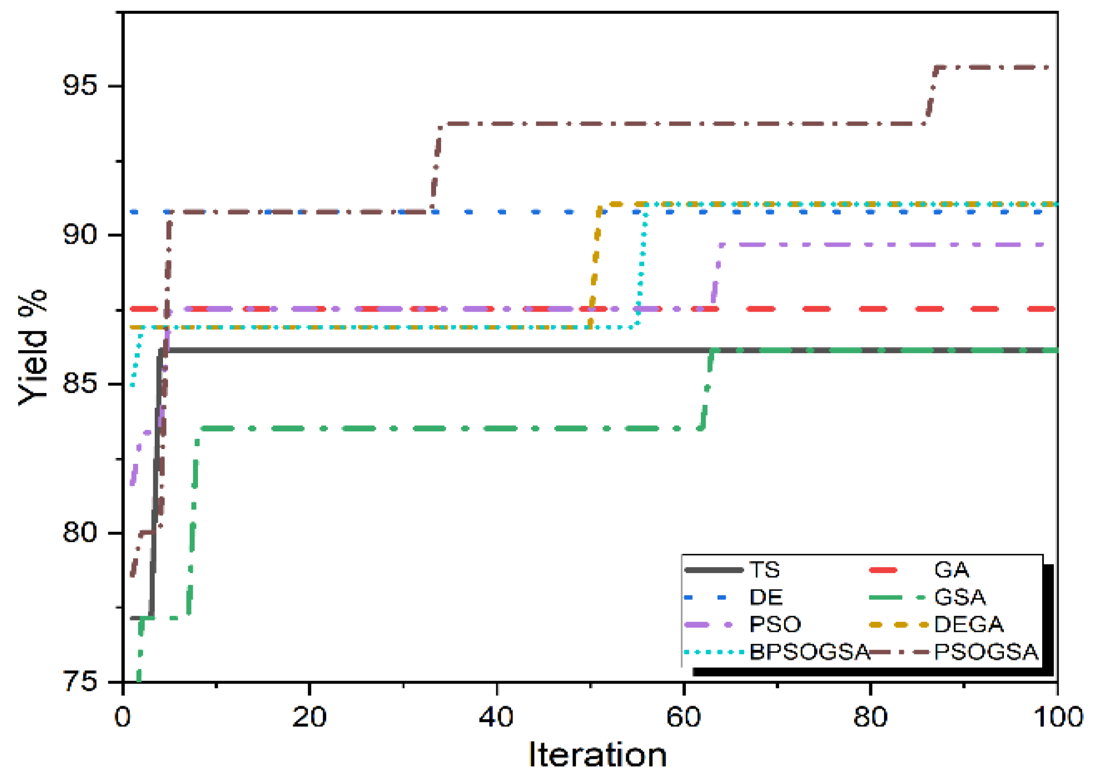
In this article, the optimal process parameters to maximize the palm oil yield are analyzed using TS, GA, DE, GSA, PSO, DEGA, BPSOGSA and PSOGSA optimizers. The optimization is performed considering 30 search agents and a maximum iteration of 100. The convergence curves of yield % for TS, GA, DE, GSA, PSO, DEGA, BPSOGSA and PSOGSA optimizers are shown in Figure 1.
From 
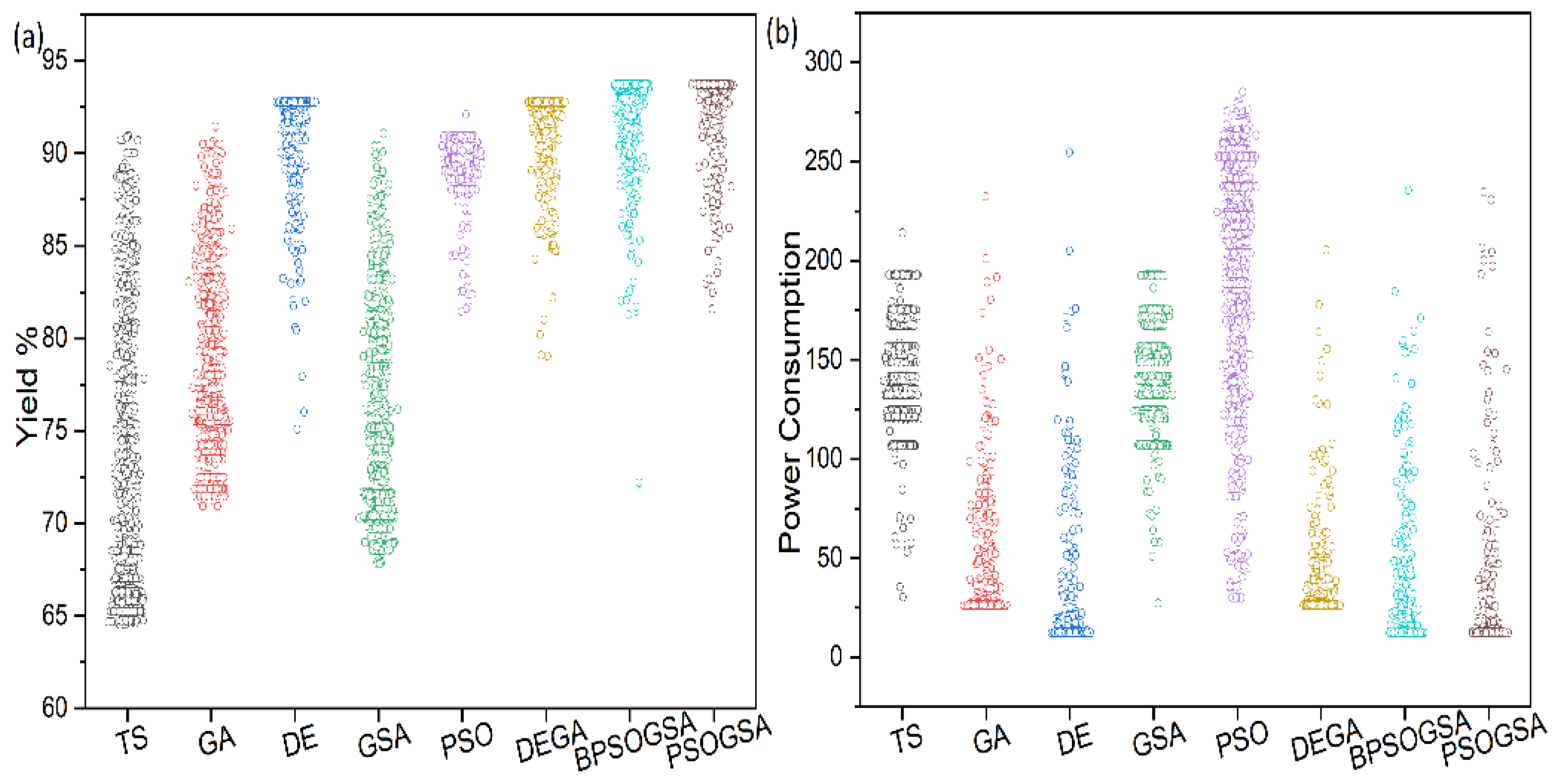
Figure 1, it is seen that for GA and DE, there is no improvement in its best value even after 100 iterations. TS and GSA require very few iterations to locate their personal best values, which appear to be the local optima. DEGA and BPSOGSA have similar performance in terms of convergence to their respective best value. PSOGSA, on the other hand, shows stepwise improvement in its best solution over the iterations. It converges at the best optimal value found so far by all the algorithms. The distribution of 3000 functional evaluation values for TS, GA, DE, GSA, PSO, DEGA, BPSOGSA and PSOGSA is presented in Figure 2. From these scatters, it is observed that GSA, PSO, BPSOGSA and PSOGSA have a maximum number of evaluated function values in the mid-range region. Further, PSOGSA appears to have reached the best-known function value very few times. DEGA shows a good overall distribution of the evaluated function values.
For unbiased comparisons, each algorithm is independently run for 10 times. The performance analysis (best value, worst value, mean value, median value, and standard deviation value) of TS, GA, DE, GSA, PSO, DEGA, BPSOGSA and PSOGSA optimizers is presented in Table 1. From Table 1, it is seen that the maximum best value of yield is obtained by the PSOGSA algorithm (i.e., 95.646). Among the eight algorithms, PSOGSA generates better results than TS, GA, DE, GSA, PSO, DEGA and BPSOGSA. In PSOGSA, the functional values lie between 91.055 and 95.646, with a mean value of 93.455 and median value of 93.750. However, the standard deviation is the minimum for DE (i.e., 0.238) and low for BPSOGSA (i.e., 0.287).
Optimal values of process parameters and response using TS, GA, DE, GSA, PSO, DEGA, BPSOGSA and PSOGSA are presented in Table 2. The obtained results are compared with the previously published results by Ayoub et al. [31]. The maximum yield values are improved by 11.75%, 11.64%, 15.98%, 11.98%, 14.41%, 16.14%, 16.14% and 22.00% using TS, GA, DE, GSA, PSO, DEGA, BPSOGSA and PSOGSA, respectively. The PSOGSA optimizer gives the greatest improvement (i.e., 22.00%) on the previous known yield value.

4. Case Study 2: Multi-Objective Process Optimization for Biodiesel Production

Mostafaei et al. [32] used the response surface methodology (RSM) to optimize the ultrasonic-assisted continuous biodiesel production from waste cooking oil. They used CCD to design 50 experimental runs, using a combination of five process parameters. The process parameters were irradiation distance ( x 1 ), UP amplitude ( x 2 ), prob diameter ( x 3 ), vibration pulse ( x 4 ) and flow rate ( x 5 ). The responses considered were yield ( R 1 ) and energy consumption ( R 2 ). It should be noted that the objective is to maximize yield ( R 1 ) and minimize energy consumption ( R 2 ). The true range of the process parameters was considered to be 30 to 90 mm for x 1 , 20% to 100% for x 2 , 14 to 42 mm for x 3 , 20% to 100% for x 4 and 40 to 80 mL/min for x 5 . However, the process parameters are coded as −2 to +2, and the following mathematical model for yield ( R 1 ) and energy consumption ( R 2 ) is used.
R 1 = 90.14 + 0.6275 x 1 + 0.8975 x 2 + 0.6125 x 3 + 0.6975 x 4 0.5325 x 5 0.428125 x 1 x 2 + 0.353125 x 1 x 4 0.296875 x 2 x 3 0.571875 x 2 x 4 + 0.509375 x 2 x 5 0.178125 x 3 x 4 + 0.665625 x 4 x 5 1.035625 x 2 2 0.985625 x 3 2 1.248125 x 4 2 + 0.214375 x 5 2
R 2 = 120.3575 10.2975 x 1 + 18.4825 x 2 + 29.3425 x 3 + 14.6175 x 4 0.032499 x 5 1.321875 x 1 x 2 2.509375 x 1 x 3 + 0.646875 x 1 x 5 + 3.921875 x 2 x 3 + 2.409375 x 2 x 4 1.021875 x 2 x 5 + 3.884375 x 3 x 4 + 0.590625 x 4 x 5 3.428125 x 1 2 + 0.809375 x 2 2 0.965625 x 3 2
In this case study, the maximization of yield % ( R 1 ) and minimization of power consumption ( R 2 ) using TS, GA, DE, GSA, PSO, DEGA, BPSOGSA and PSOGSA is carried out. The convergence curve of yield % and power consumption with the iterations is shown in Figure 3. The optimization is performed considering 30 search members and maximum iterations of 100. Figure 3a shows that despite the maximization of yield %, GSA and PSO did not show any improvement in the best value as the iterations progressed. On the other hand, the three remaining traditional algorithms, i.e., TS, GA and DE, converged to their respective best value in the 12th, 7th and 15th iterations. The hybrid algorithms, i.e., DEGA, BPSOGSA and PSOGSA, converged to their respective best values in the 13th, 9th and 8th iterations. Thus, for the yield % objective, all the functions recorded very fast convergence to their respective best values. Nevertheless, it is worth mentioning that, except BPSOGSA and PSOGSA, all the other algorithms converged to relatively poorer solutions. A similar trend is observed in Figure 3b, where convergence characteristics of the tested algorithm in the power consumption minimization scenario are reported. However, here, the DE, DEGA, BPSOGSA and PSOGSA all were able to locate the best-known optimum, which may be the global optimum.
Scatter of the 3000 function evaluation values for TS, GA, DE, GSA, PSO, DEGA, BPSOGSA and PSOGSA is presented in Figure 4. It is seen that the distribution pattern of DE, PSO, DEGA, BPSOGSA and PSOGSA is somewhat similar. Major accumulations of function evaluation values are seen to be clustered in the higher yield % zone. On the other hand, the other three algorithms, i.e., TS, GA and GSA, showed throughout the distribution of the function evaluation values. Similar observations are made from Figure 4b, where GA, DE, GSA, DEGA, BPSOGSA and PSOGSA showed good concentrations of solutions in the lower power consumption zone, indicating that the algorithms spent a relatively smaller number of function evaluations to locate the potential global optimal zone.
Table 3 presents the optimal process parameters and the achieved best value for yield % optimization by the eight algorithms. It is observed that both BPSOGSA and PSOGSA were able to achieve the maximum yield % (i.e., 93.715). All the algorithms were able to locate good solutions for yield % maximization. Similarly, from Table 4, it is seen that all the three hybrid algorithms, i.e., DEGA, BPSOGSA and PSOGSA, as well as DE were able to locate the best-known minimum power consumption value (i.e., 12.48).
The ability of the hybrid algorithms to tackle multi-objective optimization problems is also assessed by considering a weighted sum multi-objective optimization wherein yield % and power consumption are simultaneously optimized. The composite objective function Z is described as
Min   Z = 0.5 R 2 R 2 min 0.5 R 1 R 1 max
where R 1 max and R 2 min are the best-known values of yield % and power consumption single-objective optimization.
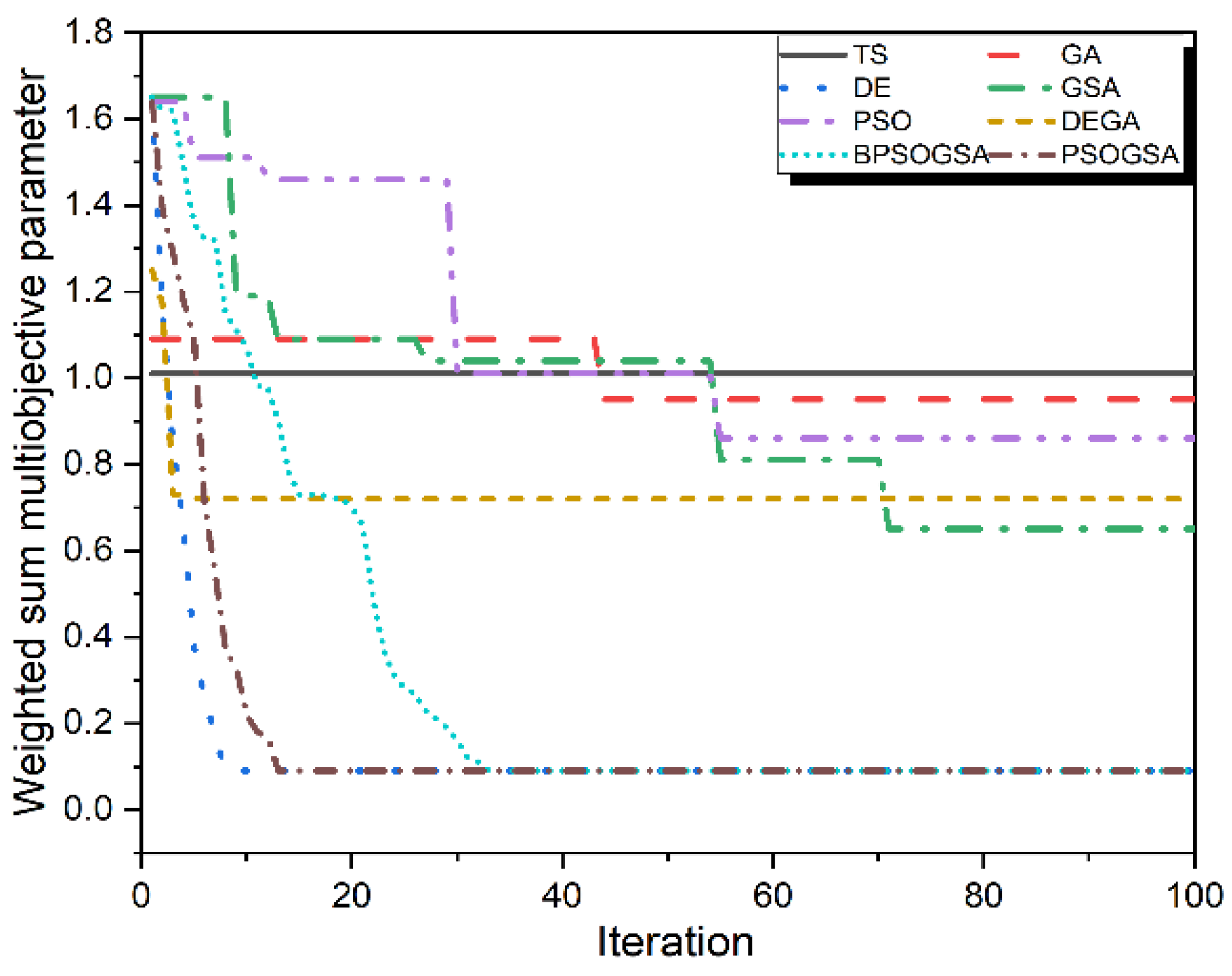
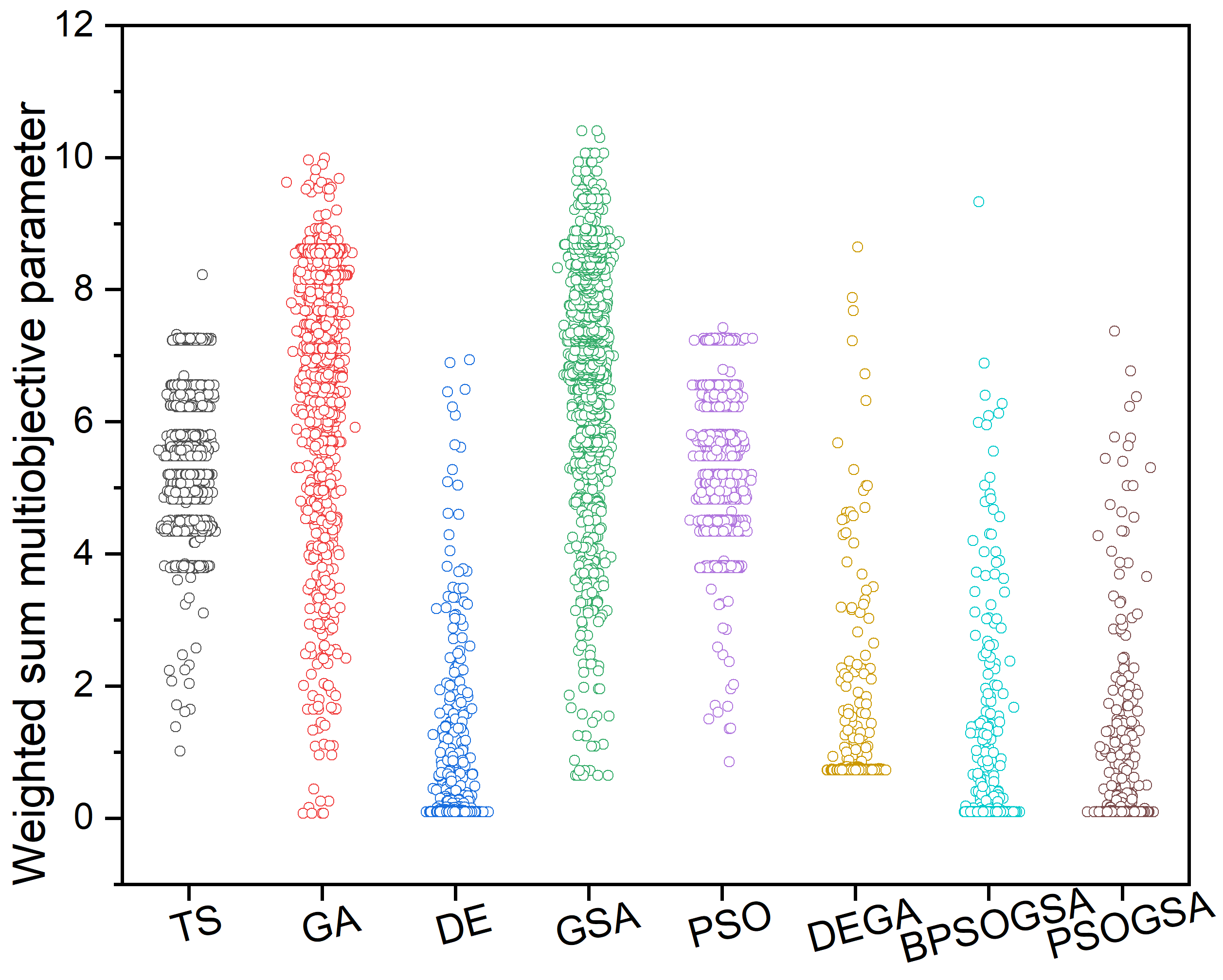
The convergence of multi-objective function with respect to iteration and distribution scatter of 3000 function evaluations for TS, GA, DE, GSA, PSO, DEGA, BPSOGSA and PSOGSA is presented in Figure 5 and Figure 6, respectively.
The performance analysis of the eight optimizers in the weighted sum multi-objective environment is given in Table 5. In multi-objective optimization, the minimum value of the function is obtained using PSOGSA, whereas for DEGA and BPSOGSA, the obtained solution is almost on par with that of PSOGSA.
The optimal process parameters and responses are presented in Table 6. The obtained results are compared with the previously published results by Mostafaei et al. [32]. The optimal result is improved about 72.12%, 73.77%, 80.03%, 82.20%, 76.45%, 97.49%, 97.49% and 97.52% using TS, GA, DE, GSA, PSO, DEGA, BPSOGSA and PSOGSA, respectively. However, it is important to state here that the derived multi-objective results are dependent on the considered weightage of the objectives. The composite objective function Z is a compromise solution that takes into account both yield ( R 1 ) and energy consumption ( R 2 ). This is why in the best solution derived by PSOGSA, the R 1 dropped by about 15.7% whereas the R 2 improved by approximately 88%. The average computational time for each independent run of TS, GA, DE, GSA, PSO, DEGA, BPSOGSA and PSOGSA is 2.010, 2.351, 2.411, 3.832, 2.407, 3.973, 4.771 and 4.684 s, respectively.

5. Conclusions

To improve the performance and capabilities of industrial processes, it is crucial to optimize them. Most industrial processes are combinatorial optimization problems, where the performance or responses can be significantly improved by assigning optimized values to each process parameter. In this study, based on the two independent case studies on biodiesel production optimization, the following conclusions regarding the hybrid algorithms can be drawn.
  • For case study 1, the tested algorithms can be ranked as PSOGSA > DEGA > BPSOGSA > DE > PSO > GSA > TS > GA based on best solution and mean solution. For case study 2, considering all the three scenarios (i.e., yield % maximization, power consumption minimization and weighted sum multi-objective minimization), the ranking is PSOGSA > BPSOGSA > DEGA > DE > GSA > GA > PSO > TS. Thus, in terms of quality of the optimum obtained, PSOGSA, BPSOGSA and DEGA are the top three algorithms. However, in general, PSOGSA is found to be roughly 1–2% better than BPSOGSA and DEGA for the tested case studies.
  • Based on variance in the optimum, the algorithms can be ranked from least variance to most variance as DEGA > DE > BPSOGSA > PSO > TS > GSA > PSOGSA > GA for case study 1. For case study 2, the ranking is DE > PSOGSA > TS > BPSOGSA > GSA > GA > PSO > DEGA. Using an average ranking methodology and considering both case studies 1 and 2, the top three algorithms (i.e., lesser variance) are DE, BPSOGSA and TS.
  • In terms of computational time, the hybrid algorithms are slower than their traditional counterparts. The algorithms can be ranked from fastest to slowest as TS > GA > PSO > DE > GSA > DEGA > PSOGSA > BPSOGSA. With respect to TS, the GA, DE, GSA, PSO, DEGA, BPSOGSA and PSOGSA are found to be 17%, 20%, 20%, 91%, 98%, 133% and 137% slower, respectively.
  • With regards to the previous best known solution from the literature, the traditional algorithms improved the solution by an average of 13.15%, whereas the hybrid algorithm improved it by 18.09% for case study 1. Similarly, for case study 2, the improvements were seen to be 76.91% and 97.5% for traditional and hybrid algorithms, respectively.
Polynomial regression models are quite common in industrial process optimization research studies and applications. The outcomes of this study will be beneficial to any similar study that relies on second-order models. This study can be further improved by considering the probabilistic and non-probabilistic uncertainties of process parameters. Hybridization of the metaheuristics with MCDMs for multi-objective optimization is also likely to lead toward some interesting research.

Author Contributions

Conceptualization, R.S., N.G., R.Č., R.C.N. and K.K.; data curation, S.P.; formal analysis, S.P. and K.K.; methodology, R.S., N.G., R.Č. and R.C.N.; project administration, R.Č.; resources, R.S., N.G., R.Č. and R.C.N.; software, R.S., N.G. and R.C.N.; supervision, R.Č.; validation, S.P. and K.K.; visualization, S.P. and K.K.; writing—original draft, R.S., N.G., R.C.N. and S.P.; writing—review and editing, R.Č. and K.K. All authors have read and agreed to the published version of the manuscript.

Funding

This research received no external funding.

Institutional Review Board Statement

Not applicable.

Informed Consent Statement

Not applicable.

Data Availability Statement

The data presented in this study are available through email upon request to the corresponding author.

Conflicts of Interest

The authors declare no conflict of interest.

Appendix A

Algorithm A1: Pseudocode of PSO
  Inputs:   Population size (N), tmax (Max. iteration number)
  Initialize the random population (N), and initial random velocity (v)
  Evaluate the objective function values of N.
  Assign Pbest and fpbest
  Select the gbest and fgbest
  while (t < tmax)
     for t = 1   to N
       Determine the velocity ( v i ) of ith particle
       Determine the position ( X i ) of ith particle
       Bound  X i
       Evaluate the objective values of ith particle
           if  current fitness values are better than the older one
             then  update Pbest and fpbest
           End
           if  current fitness value is better among the entire population
            then   update gbest and fgbest
           End
     End
     t = t + 1
  End
  Return the best solution
Algorithm A2: Pseudocode of GSA
  Inputs: Population size (N), Max. iteration number (tmax)
  while (t < tmax)
     Evaluate the fitness for each agent
     Update the G, best and worst of the population
     Calculate M and a for each agent
     Update velocity and position
  End
  t = t + 1
  Return the best solution

References

  1. Yong-Jie, M.; Wen-Xia, Y. Research progress of genetic algorithm. Appl. Res. Comput. 2012, 29, 1201–1206. [Google Scholar]
  2. Eberhart, R.; Kennedy, J. Particle swarm optimization. In Proceedings of the IEEE International Conference on Neural Networks, Perth, WA, Australia, 27 November–1 December 1995; Volume 4, pp. 1942–1948. [Google Scholar]
  3. Karaboga, D. Artificial bee colony algorithm. Scholarpedia 2010, 5, 6915. [Google Scholar] [CrossRef]
  4. Yang, X.S.; He, X. Bat algorithm: Literature review and applications. Int. J. Bio-Inspired Comput. 2013, 5, 141–149. [Google Scholar] [CrossRef] [Green Version]
  5. Rashedi, E.; Nezamabadi-pour, H.; Saryazdi, S. GSA: A Gravitational Search Algorithm. Inf. Sci. 2009, 179, 2232–2248. [Google Scholar] [CrossRef]
  6. Dorigo, M.; Blum, C. Ant colony optimization theory: A survey. Theor. Comput. Sci. 2005, 344, 243–278. [Google Scholar] [CrossRef]
  7. Price, K.V. Differential Evolution. In Handbook of Optimization; Springer: Berlin/Heidelberg, Germany, 2013; pp. 187–214. [Google Scholar] [CrossRef]
  8. Mirjalili, S. The ant lion optimizer. Adv. Eng. Softw. 2015, 83, 80–98. [Google Scholar] [CrossRef]
  9. Mirjalili, S.; Mirjalili, S.M.; Hatamlou, A. Multi-Verse Optimizer: A nature-inspired algorithm for global optimization. Neural Comput. Appl. 2016, 27, 495–513. [Google Scholar] [CrossRef]
  10. Mirjalili, S.; Gandomi, A.H.; Mirjalili, S.Z.; Saremi, S.; Faris, H.; Mirjalili, S.M. Salp Swarm Algorithm: A bio-inspired optimizer for engineering design problems. Adv. Eng. Softw. 2017, 114, 163–191. [Google Scholar] [CrossRef]
  11. Faris, H.; Aljarah, I.; Al-Betar, M.A.; Mirjalili, S. Grey wolf optimizer: A review of recent variants and applications. Neural Comput. Appl. 2018, 30, 413–435. [Google Scholar] [CrossRef]
  12. Mirjalili, S. Dragonfly algorithm: A new meta-heuristic optimization technique for solving single-objective, discrete, and multi-objective problems. Neural Comput. Appl. 2016, 27, 1053–1073. [Google Scholar] [CrossRef]
  13. Mirjalili, S.; Lewis, A. The Whale Optimization Algorithm. Adv. Eng. Softw. 2016, 95, 51–67. [Google Scholar] [CrossRef]
  14. Yang, X.S.; He, X. Firefly algorithm: Recent advances and applications. Int. J. Swarm Intell. 2013, 1, 36–50. [Google Scholar] [CrossRef] [Green Version]
  15. Kuo, R.J.; Lin, L.M. Application of a hybrid of genetic algorithm and particle swarm optimization algorithm for order clustering. Decis. Support Syst. 2010, 49, 451–462. [Google Scholar] [CrossRef]
  16. Mafarja, M.M.; Mirjalili, S. Hybrid Whale Optimization Algorithm with simulated annealing for feature selection. Neurocomputing 2017, 260, 302–312. [Google Scholar] [CrossRef]
  17. Zhang, Z.; Ding, S.; Jia, W. A hybrid optimization algorithm based on cuckoo search and differential evolution for solving constrained engineering problems. Eng. Appl. Artif. Intell. 2019, 85, 254–268. [Google Scholar] [CrossRef]
  18. Guo, J.; Sun, Z.; Tang, H.; Jia, X.; Wang, S.; Yan, X.; Ye, G.; Wu, G. Hybrid Optimization Algorithm of Particle Swarm Optimization and Cuckoo Search for Preventive Maintenance Period Optimization. Discret. Dyn. Nat. Soc. 2016, 2016, 1516271. [Google Scholar] [CrossRef] [Green Version]
  19. Radosavljević, J.; Klimenta, D.; Jevtić, M.; Arsić, N. Optimal Power Flow Using a Hybrid Optimization Algorithm of Particle Swarm Optimization and Gravitational Search Algorithm. Electr. Power Compon. Syst. 2015, 43, 1958–1970. [Google Scholar] [CrossRef]
  20. Betiku, E.; Okunsolawo, S.S.; Ajala, S.O.; Odedele, O.S. Performance evaluation of artificial neural network coupled with generic algorithm and response surface methodology in modeling and optimization of biodiesel production process parameters from shea tree (Vitellaria paradoxa) nut butter. Renew. Energy 2015, 76, 408–417. [Google Scholar] [CrossRef]
  21. Garg, A.; Jain, S. Process parameter optimization of biodiesel production from algal oil by response surface methodology and artificial neural networks. Fuel 2020, 277, 118254. [Google Scholar] [CrossRef]
  22. Miraculas, G.A.; Bose, N.; Raj, R.E. Process parameter optimization for biodiesel production from mixed feedstock using empirical model. Sustain. Energy Technol. Assess. 2018, 28, 54–59. [Google Scholar] [CrossRef]
  23. Patil, P.D.; Deng, S. Optimization of biodiesel production from edible and non-edible vegetable oils. Fuel 2009, 88, 1302–1306. [Google Scholar] [CrossRef]
  24. Outili, N.; Kerras, H.; Nekkab, C.; Merouani, R.; Meniai, A.H. Biodiesel production optimization from waste cooking oil using green chemistry metrics. Renew. Energy 2020, 145, 2575–2586. [Google Scholar] [CrossRef]
  25. Ghadai, R.K.; Kalita, K.; Mondal, S.C.; Swain, B.P. Genetically optimized diamond-like carbon thin film coatings. Mater. Manuf. Process. 2019, 34, 1476–1487. [Google Scholar] [CrossRef]
  26. Singh, A.; Ghadai, R.K.; Kalita, K.; Chatterjee, P.; Pamučar, D. EDM process parameter optimization for efficient machining of Inconel-718. Facta Univ. Ser. Mech. Eng. 2020, 18, 473–490. [Google Scholar] [CrossRef]
  27. Mahmood, M.A.; Popescu, A.C.; Oane, M.; Channa, A.; Mihai, S.; Ristoscu, C.; Mihailescu, I.N. Bridging the analytical and artificial neural network models for keyhole formation with experimental verification in laser melting deposition: A novel approach. Results Phys. 2021, 26, 104440. [Google Scholar] [CrossRef]
  28. Mahmood, M.A.; Visan, A.I.; Ristoscu, C.; Mihailescu, I.N. Artificial neural network algorithms for 3D printing. Materials 2021, 14, 163. [Google Scholar] [CrossRef]
  29. Mirjalili, S.; Hashim, S.Z.M. A new hybrid PSOGSA algorithm for function optimization. In Proceedings of the 2010 International Conference on Computer and Information Application, Tianjin, China, 3–5 December 2010; pp. 374–377. [Google Scholar]
  30. Mirjalili, S.; Wang, G.G.; Coelho, L.D.S. Binary optimization using hybrid particle swarm optimization and gravitational search algorithm. Neural Comput. Appl. 2014, 25, 1423–1435. [Google Scholar] [CrossRef]
  31. Ayoub, M.; Ullah, S.; Inayat, A.; Bhat, A.H.; Hailegiorgis, S.M. Process Optimization for Biodiesel Production from Waste Frying Oil over Montmorillonite Clay K-30. Procedia Eng. 2016, 148, 742–749. [Google Scholar] [CrossRef] [Green Version]
  32. Mostafaei, M.; Ghobadian, B.; Barzegar, M.; Banakar, A. Optimization of ultrasonic assisted continuous production of biodiesel using response surface methodology. Ultrason. Sonochem. 2015, 27, 54–61. [Google Scholar] [CrossRef]
Figure 1. Convergence curve of GSA, PSO, BPSOGSA and PSOGSA.
Processes 10 00616 g001
Figure 2. Total function evaluations during a typical optimization run.
Processes 10 00616 g002
Figure 3. Convergence curve of various metaheuristics while optimizing (a) yield % (b) power consumption.
Processes 10 00616 g003
Figure 4. Distribution of total evaluated functions for various metaheuristics while optimizing (a) yield %, (b) power consumption.
Processes 10 00616 g004
Figure 5. Convergence curve of algorithms for multi-objective optimization.
Processes 10 00616 g005
Figure 6. Scatter of total evaluated functions of algorithms for multi-objective optimization.
Processes 10 00616 g006
Table 1. Performance of GSA, PSO, BPSOGSA and PSOGSA.
OptimizerBestWorstMeanMedianStandard Deviation
TS87.61483.68785.67586.0171.354
GA87.52982.05785.02285.6132.188
DE90.93090.18890.53990.5120.238
GSA87.79683.52086.13886.1431.441
PSO89.69787.51488.14787.5290.833
DEGA91.05590.78690.89090.7860.130
BPSOGSA91.05590.08290.72490.7860.287
PSOGSA95.64691.05593.45593.7501.520
Table 2. Optimal process parameter and responses.
OptimizerReaction TimeReaction TempCatalyst AmountRatio O/MYield %Improvement %
Ayoub et al. [31]180.0090.003.001:1278.4-
TS75.00101.004.871:1187.61411.75%
GA75.00101.004.871:1087.52911.64%
DE97.20109.254.461:890.93015.98%
GSA148.80103.754.881:987.79611.98%
PSO262.80108.754.861:789.69714.41%
DEGA196.80120.004.791:691.05516.14%
BPSOGSA196.80120.004.791:691.05516.14%
PSOGSA66.60125.004.791:795.64622.00%
Table 3. Optimal process parameter for optimization of yield %.
Optimizer x 1 x 2 x 3 x 4 x 5 Response
TS77.2579.431.3657.843.290.938
GA84.658.423.3859.24491.731
DE906429.3380.88092.768
GSA8771.626.3272.847.791.07
PSO86.5543.432.4173.847.792.08
DEGA906429.3380.88092.768
BPSOGSA9048.830.6662.64093.715
PSOGSA9048.830.6662.64093.715
Table 4. Optimal process parameter for optimization of power consumption.
Optimizer x 1 x 2 x 3 x 4 x 5 Response
TS86.722.617.8530.462.130.223
GA302014208026.34
DE902014204012.48
GSA76.6525.414.1422.442.927.225
PSO85.6529.417.0842.244.229.982
DEGA902014204012.48
BPSOGSA902014204012.48
PSOGSA902014204012.48
Table 5. Performance of metaheuristics in multi-objective optimization.
OptimizerBestWorstMeanMedianStandard
Deviation
TS1.0121.6441.4541.6440.290
GA0.9521.6441.3581.4470.304
DE0.7251.2501.0931.2500.241
GSA0.6461.2501.0081.2500.296
PSO0.8551.6441.0920.8550.316
DEGA0.0911.4590.7750.7750.684
BPSOGSA0.0910.7250.2810.0910.291
PSOGSA0.0900.7250.2170.0910.254
Table 6. Optimal process parameter for multi-objective optimization.
Optimizer x 1 x 2 x 3 x 4 x 5 Z R 1 R 2 %   Improvement   in   Z
Mostafaei et al. [32]75562862503.63091.6102.8-
TS8420.214.4978.8761.01281.17936.25672.12%
GA88.85616.2446.843.30.95288.04435.45173.77%
DE30201420800.72561.99826.3480.03%
GSA86.227.617.5726.444.70.64681.01826.94082.20%
PSO85.573.414.6322.441.90.85583.01332.49776.45%
DEGA90201421.6400.09177.15512.54897.49%
BPSOGSA90201420400.09176.63812.48097.49%
PSOGSA90201421.6400.09077.15512.54897.52%
Publisher’s Note: MDPI stays neutral with regard to jurisdictional claims in published maps and institutional affiliations.

