Article

A Multicriteria Decision Trading System Based on Prospect Theory: A Risk Return Analysis of the TODIM Method

1
Postgraduate Program in Operations Research, Instituto Tecnológico de Aeronáutica (CEP 12228-900), Universidade Federal de São Paulo, São Paulo 04021-001, Brazil
2
Departamento de Tecnologia, Universidade Federal de São João Del-Rei, São João Del-Rei 36307-352, Brazil
3
Departamento de Engenharia Eletrônica, Universidade Federal de Minas Gerais, Belo Horizonte 31270-901, Brazil
4
Instituto Tecnológico de Aeronáutica, São Paulo 12228-900, Brazil
*
Author to whom correspondence should be addressed.
Processes 2022, 10(3), 609; https://doi.org/10.3390/pr10030609
Submission received: 31 January 2022 / Revised: 16 February 2022 / Accepted: 22 February 2022 / Published: 21 March 2022

Abstract

:
This paper proposes a trading system (TS) based on a multicriteria decision aid (MCDA) process known as TODIM, (Multicriteria Interactive Decision Making) a Portuguese acronym for interactive and multicriteria decision-making. MCDA has been employed to solve financial questions because of its ability to deal with a complex environment populated with different sorts of criteria and alternatives, such as financial markets. The aim is to propose a general and adaptive tool for supporting the trading strategies of investors and market practitioners in such an environment. The reason for selecting TODIM among the different MCDA methods is that it is based on prospect theory, which assumes that the risk profile of the investor varies according to different situations, considering the risk of loss or gain. A list of simulations using some of the most prominent Brazilian stocks is performed, and the results are compared with the Buy-and-Hold benchmark and a TS based on an ensemble method for selecting trading rules. The results show that, compared to Buy-and-Hold, a TODIM-based TS provides the same level of return with a lower level of risk exposure. The consequence is superior risk adjustment parameters. As a result, we have a model with similar results in profit, but with superior results in relation to risk-based performance, which makes the method advantageous in relation to similar ones.

1. Introduction

Many theories from traditional finance are rooted in the rationality premise, constraining market agents as maximizers with consistent beliefs. For instance, the efficient market hypothesis (EMH) assumes that every investor is entirely rational and that speculative asset prices always reflect all information available [1]. A few other examples that have flourished in this ground are: arbitrage theory [2], the portfolio selection framework [3], the capital asset pricing model [4]; and option-pricing theory [5]. For an historical perspective on this subject the reader is referred to the work of [6]. Nevertheless, several anomalies, or market inefficiencies, have been reported ever since: long-run reversals, seasonal patterns, speculative bubbles, etc. Even in the seminal work of [1] slight serial dependencies in returns were reported, even though understated.
Several studies (e.g., [7,8,9,10]) have criticized or relaxed the tenets that every agent in the market is a rational optimizer, and argue that decision-makers that maximize linear expected utility—a premise of the neoclassical microeconomic theory [11]—are unrealistic in real-world circumstances. Indeed, human behavior is guided by simplified procedures or heuristics [8]. The main argument is that in a real-world situation, due to the limited capacity of investors, agents are unable to obtain and optimally analyze all relevant information; they thus face cruel difficulties in solving complex problems and issues. In addition, investors face difficulties in compiling a comprehensive list of alternative courses of action and determining and assigning values and probabilities to each of many possible courses of action. Because of these aspects they are forced to rely on heuristics which in some circumstances result in good decisions and performance, but not in all situations.
Behavioral finance [12] has emerged as a compelling theory seeking to bridge the gap between traditional finance on the one hand and psychology and sociology on the other to explain how and why markets, and ultimately agents, behave as they do. This theory is intended to shed light on the investment decision-making process of real people, based on cognitive psychology and biases related to investors beliefs [10,13,14]. A recent survey in [15] studied 25 profiling characteristics associated with risk-aversion in a sample of a national population in the UK, including some characteristics not previously investigated in the literature. A noticeable loss aversion is reported, correlated with many of the investigated characteristics and substantially different for the subset of graduate students, a social group normally used in other research. In a natural experiment, the entry of domestic individual investors in the B-share market in China, from 2001 onward, was investigated in [16], showing that this type of investors is more prone to framing bias than the institutional decision-makers. Evidence of investors using the historical returns distribution of stocks as a proxy of future pricing instead of trying to predict the actual future value are laid out in [17]. The influence of cultural aspects concerning this hypothesis is further investigated in [18] for emerging markets.
To operate in financial markets, an alternative to discretionary trading is based on the trading system (TS), in which investments are made objectively using so-called technical trading rules (TTRs) [19] or quantitative trading [20] to support the decision-making process. In short, a trading system aggregates some input signals and, based on a set of parameters and algorithms, creates buy/sell recommendations of a given security as outputs [21].
Even in this more systematic scenario, there are many variables to consider. As data size and number of attributes are increasing in finance-related applications, the need to extract value from data grows proportionally. This relevance is shown by [22] in a survey of numerous studies in computational intelligence for financial markets. An introduction to this theme is presented by [23], emphasizing the pitfalls of overfitting when using noisy data. These machine learning (ML) studies rely on multiple factors and leverage complex algorithms to gain insight into particular finance problems. Moreover, many studies report the challenges associated with the endless changes in markets as well the complexity of the time series. In this respect, multicriteria decision aid methods, which are based on simpler algorithms compared to the ML field, may offer useful results in a more interpretable fashion [24].
In this paper, we proposed a new TS merging technical and behavioral aspects. It uses the historic time series of securities as inputs. A pool of classic technical indicators (TI) and TTRs, comprising distinct methods and parameters sets, were employed for back-tested analysis. A group of risk-adjusted and profit-based metrics was considered to evaluate the performance. Periodically, the proposed TS used MCDA (Multiple-criteria decision-making) to reevaluate the trading model, adapting to the input, market condition and desired performance.
The innovative aspect here is the usage of TODIM [25], a Portuguese acronym for interactive and multicriteria decision-making, which is an MCDA rooted in behavioral finance, based on prospect theory [7]. The idea is to incorporate behavioral aspects in the adaptation stage of the TS, aiming towards risk reduction while keeping a profitable portfolio. The proposed TS was tested in eight stocks from Brazil, exhibiting different dynamics and having strong relevance for the market. The results were compared against a purely technical Ensemble TS, proposed by [21], and also the benchmark Buy-and-Hold. Moreover, simulations were carried out to investigate the effects of the parameters of the TODIM algorithm related to the risk aversion behavior, and are also reported in this manuscript.
This paper is organized as follows: Section 1 lays out fundamental concepts; the proposed approach and the experimental framework is detailed in Section 2, leading to the results in Section 3, which are discussed in Section 4; conclusions and future lines of work are given in Section 5.

1.1. Background

This section presents some of the theoretical background of this paper. Firstly, we review the literature on applications of MCDA to finance. Secondly, we briefly explain prospect theory; and finally, we review an MCDA method that is based on prospect theory known as TODIM and its application to finance.

1.1.1. Multicriteria Decision Aid

Multicriteria decision aid (MCDA) is an area of operational research that seeks to select the optimal alternative from a finite set of solutions by taking several attributes (multiple criteria) and their relationship into account [26]. Roughly speaking, MCDA has been used with four different aims [27]: (1) to select, classify and sort alternatives in the presence of conflicting criteria; (2) to learn through the decision-making process; (3) to find out an alternative or a set of alternatives that present themselves as a set of solutions to the problem; and (4) to clarify the decision.
Different authors have proposed the use of MCDA to solve financial problems. For instance, [28] reviews the literature of MCDA applications in finance. His work argues that there are three different areas of interest for the application of MCDA to finance: capital budgeting, corporate financing and financial investment, which is the purpose of this work. According to these authors, the main reason for applying MCDA to finance is that traditional financial theory has been challenged for largely using a single-criterion approach.
As data size and the number of attributes are increasing in finance-related applications, the need to extract value from data by using multiple data attributes has increased as well. The authors of [22] contend that this is crucial for extracting value from data by using multiple data attributes from a different perspective and by surveying numerous studies in computational intelligence for financial markets. These computational intelligence studies rely on multiple factors and highlight the importance of complex algorithms to gain insight into particular financial problems.
In this paper, we propose an emerging technique for MCDA known as TODIM [25]. To the best of our knowledge, this is the first paper that proposes the use of TODIM as a tool of MCDA to solve TS questions.
The reasons for using TODIM are the following. The first reason is that TODIM may be considered simpler, easier to apply and more readily comprehensible for practitioners than other MCDA methods, such as evolutionary algorithms [29]. The second reason is that this method is based on prospect theory, which has been proposed as applied to model agents’ behavior when facing different risk scenarios [30]. Finally, the last reason is that research on applications of TODIM and prospect theory have been carried out in the recent literature [29,31].

1.1.2. Prospect Theory

Briefly, prospect theory, as proposed by [7], aims at modeling the human decision-making process under risk. This theory incorporates three significant aspects to model the agent’s utility function. The first aspect is the reference dependence, i.e., agents compare their outcomes to some reference point. This means that different situations cause different agents’ reactions in the face of gains and/or losses. Further, the agent’s utility function is usually concave at the level of wealth, i.e., the utility increases as they get wealthier, but at a decreasing rate. Hence, the utility function parameters have to change the agents’ focus from levels of wealth to changes in wealth [14]. They argue that changes are the way humans experience life.
The second aspect is the concept of diminishing sensitivity. These authors argue that there is an enormous amount of wisdom about human nature captured in the S-shaped curve presented in Figure 1. The upper portion, for gains, is similar to the risk-averse utility function. However, it should be noticed that the lower portion also captures diminishing sensitivity. This is different from the standard model. The reason is that by starting from a given level, losses are captured by moving down the utility of the wealth line, meaning that each loss becomes increasingly painful. The fact that agents have diminishing sensitivity to both gains and losses has another implication. On the one hand, agents are risk-averse for gains, but on the other hand, they are risk-seeking for losses.
Finally, the third aspect is that agents are much more sensitive to losses than to gains. By examining the value function in Figure 1 at the origin, where both curves begin, it should be noticed that the loss part of the value function is steeper than the gain part: it decreases more quickly than the gain increases. Roughly speaking, losses hurt about twice as much as gains make one feel good.
Therefore, in summary, the authors of prospect theory argue that agents experience life in terms of changes. The value function is concave for gains and convex for losses. Furthermore, agents’ utility is asymmetric, because losses sting more than equivalently sized gains feel good. For an in-depth discussion of this theory, see, for instance, [7,8].

1.1.3. TODIM

Based on prospect theory, TODIM seeks to quantify the evaluation of outcomes (which are called alternatives) in three different situations (gains, indifference and loss). In summary, TODIM compares different pairs of alternatives aiming at building an outranking of them.
This method is similar to the previous MCDA method known as PROMETTHEE II [32]. However, there are two main differences between both TODIM and PROMETTHEE II. The first difference is that TODIM splits off the equation of the partial dominance matrix into a conditional equation to replicate the main concepts behind prospect theory (see Equation (1). These conditions serve to represent the situations of gains, indifference and loss, respectively.
The second difference is that TODIM incorporates a mitigation factor, θ, to the condition of losses (See Equation (1). The reason is that θ is intended to represent the different sensitivity of losses and gains as proposed by prospect theory.
TODIM works as follows. Let us suppose a matrix X = (xij) n × m in which xij indicates an alternative Ai, i = {1, 2, ⋯, n}, evaluated by a criterion Cj, j = {1, 2, ⋯, m}. Associated with each criterion Cj, there is a corresponding weight, wj, thereby forming a vector w = [w1, w2, ⋯, wj, ⋯, wm]T of the same length as vector C. In the sequence, let wcr = wc/wr be defined as the relative weight of the criterion Cc with respect to the reference criterion Cr, and wr = max {wc||c = 1, 2, ⋯, m}.
In the next step, this matrix is normalized, resulting in a transformed matrix called the matrix of partial desirabilities, P = (pij) n × m. Based on this matrix, TODIM outranks the alternatives by using the preferences expressed as the criteria weights. There are different approaches for determining these parameters [33]. In the present manuscript, however, these weights are employed as a set of parameters to be explored in our simulations. Moreover, an improved version of the original TODIM [25] has been employed in the literature (see the discussion presented by [29]). Finally, the steps performed in this method are reported in Algorithm 1. The equations used are detailed in the next sections.
Algorithm 1: The TODIM method
Input: Vector of weights, w; set of alternatives A; vector of criteria C; mitigation factor θ
Result: Ranked alternatives
Initialization: construct a matrix X; calculate P by normalization of X for all pairs (Ai,Aj), (i,j = 1, 2, ⋯, n) do
Processes 10 00609 i001
end
end
Calculate δ(Ai,Aj), using Equation (2). Calculate ξi, i ∈ {1, 2, ⋯, n} using Equation
  (3). Rank the alternatives according to ξi, i ∈ {1, 2, ⋯, n}

The Partial Dominance Matrix

Φ c   ( A i , A j ) = { w c r ( p i c p j c ) c = 1 m w c r ,   i f   p i c p j c > 0       0 ,   i f   p i c p j c = 0       1 θ w c r ( p j c p i c ) c = 1 m w c r ,   o t h e w i s e      
where Φc (Ai,Aj) indicates the partial dominance matrix given by the criterion c. In other words, the factor Φc (Ai,Aj) represents the contribution of the criterion c to the function δ (Ai,Aj) when comparing alternative i to alternative j.

The Final Dominance Matrix

The Final Dominance Matrix is given by:
δ ( A i , A j ) = c 1 m Φ c ( A i , A j ) ,   ( i , j )  

The Normalized Dominance Matrix

The Normalized Dominance Matrix is given by:
ξ i = δ ( A i , A j ) m i n δ ( A i , A j ) m a x δ ( A i , A j ) m i n δ ( A i , A j )
The alternative with the maximum value ξi, i ∈ {1, 2, ⋯, n} is the most desirable one. Therefore, the decision-maker might select it or rank all alternatives following ξi. The global value of each alternative is the result of its dominance over the others in the set. To calculate this global value, the method is based on the projections of differences in the result of the pairwise comparison of the alternatives, considering the performance of each one in the criterion referring to the reference criterion [34]. By incorporating prospect theory, the method uses an attenuation factor (θ) that allows the method to consider that the alternatives with losses have a greater absolute value compared to equal gain levels in the calculation of overall performance. Different values of θ represent different forms of the value function of prospect theory in the negative quadrant. When θ < 1, this indicates the preference behavior of a risk-averse individual, while when θ > 1 the behavior indicates an individual with more attenuated preferences concerning risk [35]. Thus, the method can incorporate in its mathematical basis the real behavior of a person in decision-making involving risks.

2. Proposed Approach

In an overview, the proposed TS aggregates many trading strategies from the literature on technical analysis (TA). Given a few risk and profit metrics (criteria), the TODIM method is used to select the best among the many trading strategies (alternatives) within a given time frame.
The trading system constantly adapts to the new incoming data, the time series of a given security. Since the relation between risk and reward varies over time according to the adaptive market hypothesis (AMH), the idea is that the continuous application of TODIM confers some adaptation capability on the proposed TS, leveraging profit and hedging risks. Similarly, an ensemble approach has been proposed by [21], comparing classical and more modern TTRs.
The proposed TS consists of two alternating stages. In the first, the same input is supplied to a set of TTRs comprising a portion of the historic time series of a given security, which is labeled as training or in-sample data. This study focuses on classical TTRs, both trend-following and range-breakout types. For a given TTR, several parameters are considered. Each TTR tries to exploit TTRs operating in parallel, simulating buy/sell decisions in a smaller portion of the in-sample data. The performance of the entire set of TTRs is evaluated according to eight performance metrics. As described in C, there are many ways to assess the performance of an investment, so that it is natural to consider distinct criteria. Then, the TODIM method is applied to outrank the TTRs and the one that guarantees the first position is selected.
In the second stage, out-of-sample or validation data is fed for the synthetic operation of the chosen TTR, emulating the result that would occur in real time. The performance of this simulated operation of the TTR within a given time frame is evaluated according to several metrics.
The validation data is concatenated with the previous training data, forming a new set of training data for the next iteration. After the initial iterations, some of the older data is discarded, keeping constant the training data size. This procedure is commonly known as walking forward.
An interesting feature of the proposed TS is an automated decision-making process for choosing a single trading strategy from a pool to operate in the market during a specific given time frame. This pool can represent an ecology of strategies competing among themselves and prioritizing some ratio of risk/reward. Prospect-theory-based models, such as TODIM, may include some of the asymmetry of the risk aversion regarding losses and gains observed by behavioral economics in the complex scenario of deciding the best trading strategy. Therefore, according to the market condition the individual failures can be minimized by changing the trading strategy, which can be very interesting from the risk-adjustment standpoint [36].
The TODIM method is non-compensatory, i.e., advantages of one attribute/criterion cannot be traded off against disadvantages of another, meaning that each attribute/criterion must stand on its own. This idea corresponds with some premises of the AMH that trading strategies are competing against each other. In TODIM, rank reversal is minimized—another advantage—because of the normalization procedure embedded in the method. Therefore, if similar market conditions reappear, a winning strategy from the past may be more likely to be selected (or to have a higher rank). This MCDA rooted in behavioral finance is the major contribution of the proposed method.
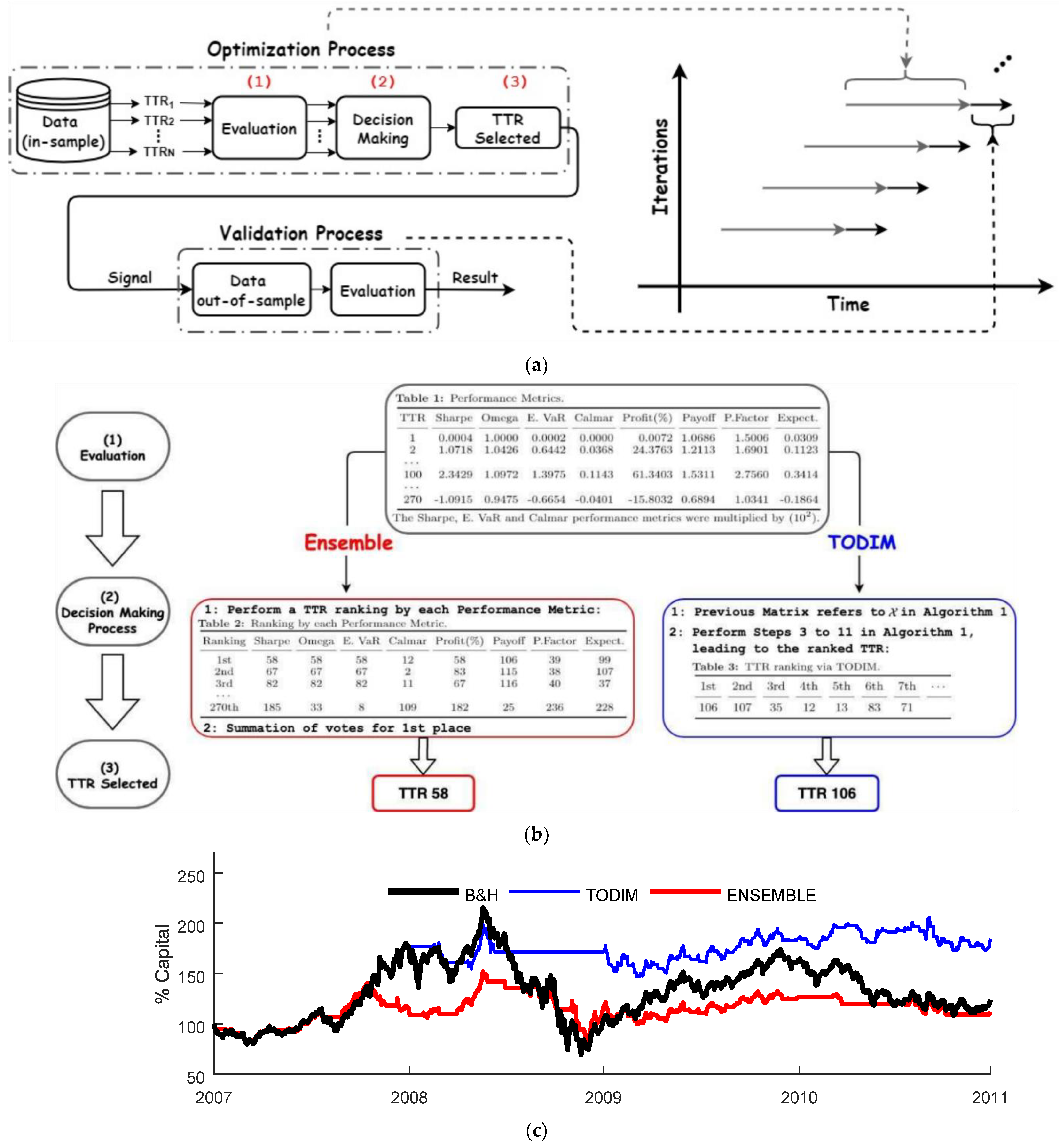
Figure 2 illustrates the key ingredients for the trading system simulation based on the walk forward method. On the left of Figure 2a, a schematic of the key steps for one iteration is presented. On the right of this figure, some iterations of the walk forward method are presented. The grey and black arrows refer to the in-sample (training) and out-of-sample (validation) dataset, respectively. Some details regarding the optimization process are provided in Figure 2b. In this Figure one can observe that, although the two methods are based on the same matrix (computed by the performance metrics evaluated for each TTR), the two multicriteria approaches might choose different TTRs at each iteration. Finally, the resulting capital curves for the first iterations of the simulated TS based on these two approaches are depicted in Figure 2c.

Experimental Framework

This investigation intends to follow neither the EMH nor the AMH in full, but rather to provide a more systematic, yet simple, framework that can be used by investors and practitioners. In this sense, these experiments are intended to analyze the benefits of using a decision-making process based on prospect theory, which is more closely related to behavioral economics, rather than a standard process less rooted in economic and financial theories. The proposed approach is compared to another TS using a distinct MCDA method, which was inspired by the ensembles method and was presented in [21]. As usual, the benchmark strategy of B&H is also compared.
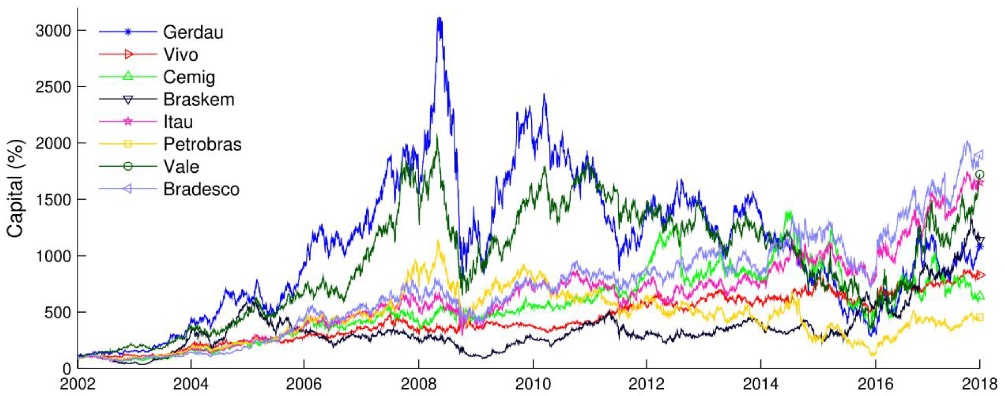
The dataset comprises the recent time series of eight major stocks from Brazil’s main stock market. The set is detailed in Appendix A.
The beginning of new presidential mandates in Brazil were used as time-stamps to divide the entire dataset into three periods: 2007–2010, 2011–2014 and 2015–2017. Moreover, an analysis of the entire dataset was performed. Therefore, there were four time frames under analysis. Only long positions were considered in the results presented; when the TS emits a sell signal, the trader does not invest the capital elsewhere.
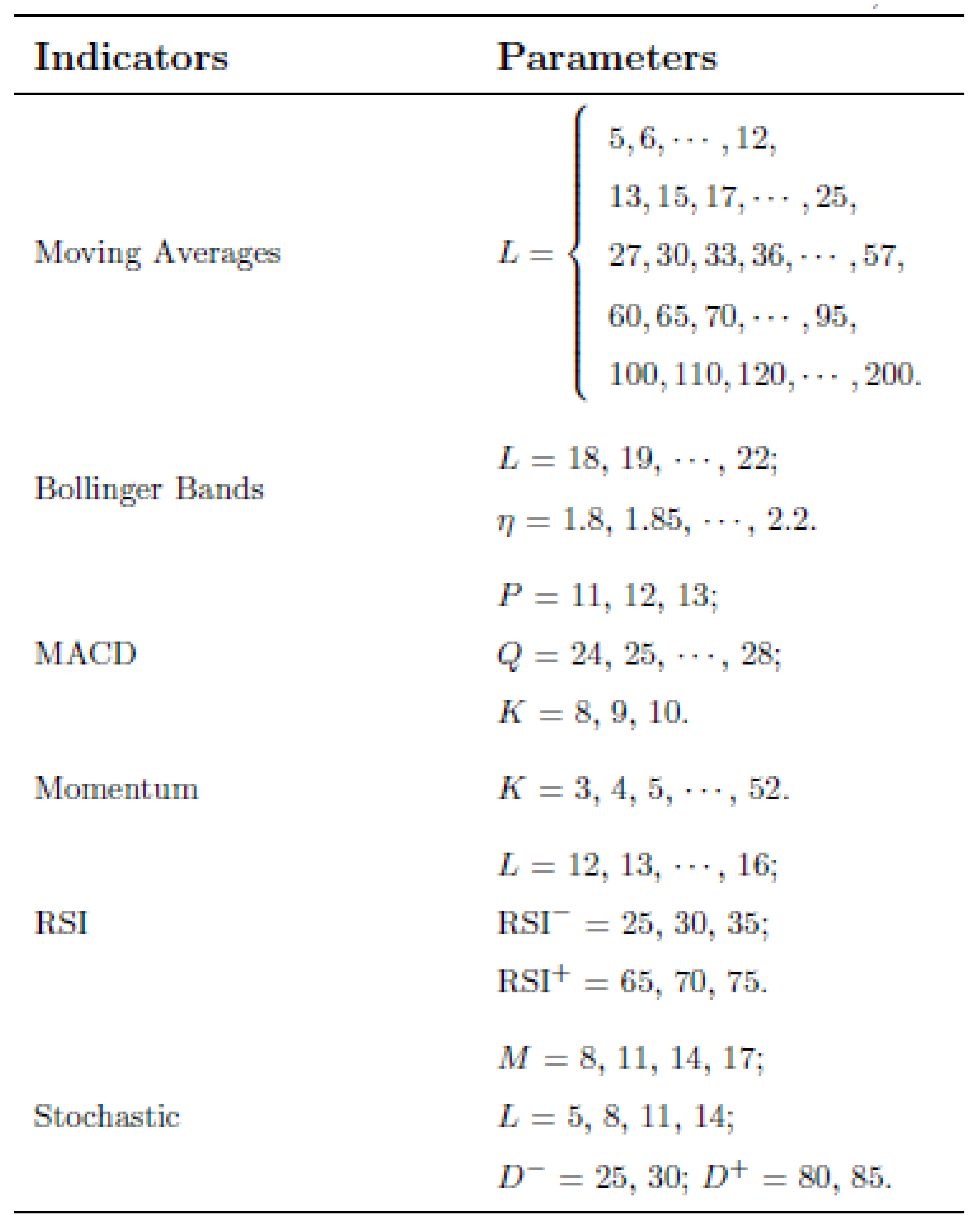
In this paper, widely used TTRs were considered, as described in Appendix B. The reason is that the emphasis is placed on the MCDA’s capacity to choose the best TTRs from a given pool of choices, instead of discussing the overall quality of the TTRs themselves.
Forecasting the power of the proposed TS and the ensemble-based TS was tested following the methodology proposed by [37] (Section 3.2). Such a test checks whether the mean returns of the proposed TS are different, with statistical relevance, from the mean return of the B&H method. The matter of risk adjustment was investigated considering the performance metrics described in Appendix C. The idea is that the returns perceived cannot be fairly measured without considering the attendant risks. In other words, if two trading strategies provide similar returns, the strategy that exposed the invested capital to lower risk is preferable. These results are presented in Section 3.1.
TODIM relies on prospect theory, which conjectures that individuals respond asymmetrically to gains and losses. This asymmetry can be quantitatively embedded in TODIM with an attenuation factor, parameter θ in Equation (1). Moreover, simulations were conducted changing the weighting factors. As this tuning may depend on the investor profile, different levels of this parameter were used in this study, as detailed in Section 3.1.1.

3. Results

This section presents experimental results comparing the proposed TS, the ensemble TS from [21] and the benchmark B&H strategy. A sensitivity analysis is also conducted for the proposed TS.

3.1. Performance Metrics

This section assumes equal weighting factors for the decision criteria (performance and risk metrics), i.e., ωrc = 0.125. Moreover, the mitigation factor is kept constant θ = 0.5.

3.1.1. Comparing the TS to the B&H Strategy

Firstly, ∆, the difference between the average return for a given TS (ṜTS) and the B&H strategy (ṜBH), is computed according to ∆ = ṜTS − ṜBH.
Table 1 reports the values of t-statistics and their respective p-values for both TS’s, considering the four time frames investigated. The returns of the proposed TS were not statistically different from those observed for the B&H strategy, except for VIVT4 during the period of 2007–2017. In a few exceptions, the returns of the ensemble TS were inferior to those observed for the B&H: BBDC4 (2007–2017), ITUB4 (2007–2017) and VIVT4 (2007–2017).
Secondly, four risk metrics were computed for all strategies. The results are compiled in Table 2. The pairwise comparison indicates that the proposed TS presented better performance than B&H for every time frame and stock, considering metrics Std. Dev., LPM and VaR. Regarding Max. DD., the proposed TS outperformed the B&H for the majority of the stocks: BRKM5, GGBR4, ITUB4, PETR4 and VALE3. For the remaining stocks, the results were mixed.
Pairwise comparison between the TSs indicates that the one based on TODIM consistently produced fewer risks. The following numbers in parentheses after each metric indicate the occurrences of a TS surpassing the other (TODIM, Ensemble): Std. Dev. (22–10); LPM (24–8); and Max. DD (24–8); and VaR (22–10). Therefore, considering 128 possible evaluations and combining distinct stocks, metrics and timeframes, the proposed TS outperformed the ensemble proposed in [21] in 71.87% of the total.

3.1.2. Comparing the TODIM TS to the Ensemble TS

In this section, the overall performance is measured by the eight proposed metrics, following the approach of [21] (Section VI). Table 3 and Table 4 report these results. Regarding the TS, the comparison for risk-adjusted metrics follows (TODIM-Ensemble): Sharpe (21-11), Omega (21-11), E. VaR (21-11) and Calmar (21-11).
Therefore, the modification proposed in the MCDA resulted in a performance that surpassed the ensemble of TTRs 65.6% of the time. Analyzing the profit-based metrics, the results are: Profit (24-8), Payoff (22-9), P. Factor (238) and Expect (23-8). The improvement of the proposed TS was larger, yielding higher metrics in 73.6% of the occasions. Combining all the metrics, the proposed TS had better performance metrics in 69.5% of the simulations.
The performance indicators (Profit, Payoff and Expect) were calculated considering a profit in relation to a loss, and the ratios of Sharpe, Omega, Calmar and E.Var were adjusted for risk. The P. Factor index is also a performance indicator, and performance is considered good when the value is greater than 1. For all the performance indicators, higher values indicate better investment performance.

3.2. Sensibility Analysis

Up to this point, the parametrization of TODIM has been kept fixed. However, it is possible to adjust θ, which measures the asymmetry in the S-shaped utility function, and ωrc, which weighs the importance of alternatives (performance metrics). This section investigates the variability of the results by the proposed TS according to changes in those parameters.
Firstly, for fixed weighting factors, the mitigation factor changed, θ = {0.1, 0.25, 0.5, 0.75, 0.9}. Table 5 and Table 6 summarize the investigation of sensitivity to θ for the time series of PETR4. Similar results were found for other iterations as well as for the other securities, but are omitted here for the sake of brevity.
Table 4 reports the first 10 TTR indexes ranked via TODIM at the first iteration of the simulation, when the mitigation factor is allowed to change. Table 5 presents the chosen TTR, i.e., the top of the ranking, for all iterations. Figure 3 depicts the empirical S-shaped curve for the Sharpe Index for a subset of values for parameter θ, given by the dominance Φc (AiAj) of Alternative Ai over Alternative Aj (Pi > Pj refers to a gain, whereas Pi < Pj indicates a loss).
Then, the mitigation factor was fixed θ = 0.5 and 100 realizations for the proposed TS were designed considering that the weighting factors were picked randomly according to a uniform distribution within the interval (0,1).
Figure 4 shows the distribution of results according to changes in the weighting factors. All performance metrics (each subfigure corresponds to a metric) are considered and each boxplot represents the simulations of security, considering the entire database. For the sake of brevity the analysis of the other time frames is omitted. The results for the ensemble-based TS are depicted as blue circles for comparison.

4. Discussion

In terms of pure profitability, none of the decision-making processes were able to stand out (Section 3.1.1). Nevertheless, the results are quite different when the returns are observed from the viewpoint of risk adjustment and performance metrics. The results show that the main contribution of this work is the proposal of a trading strategy, known as TODIM TS, that provides an identical level of returns with less risk exposition compared to the Buy-and-Hold strategy and ensemble TS. Consequently, the risk-adjustment parameters outperformed both benchmarks.
As described in Section 3.1.2, the proposed modification produces a noticeable improvement in performance in terms of risk. In approximately 70% of the scenarios investigated, the TTRs selected by TODIM outperformed those chosen by the ensemble method. This result corroborates the idea that an MCDA based on prospect theory, such as TODIM, can reflect decisions with greater risk aversion.
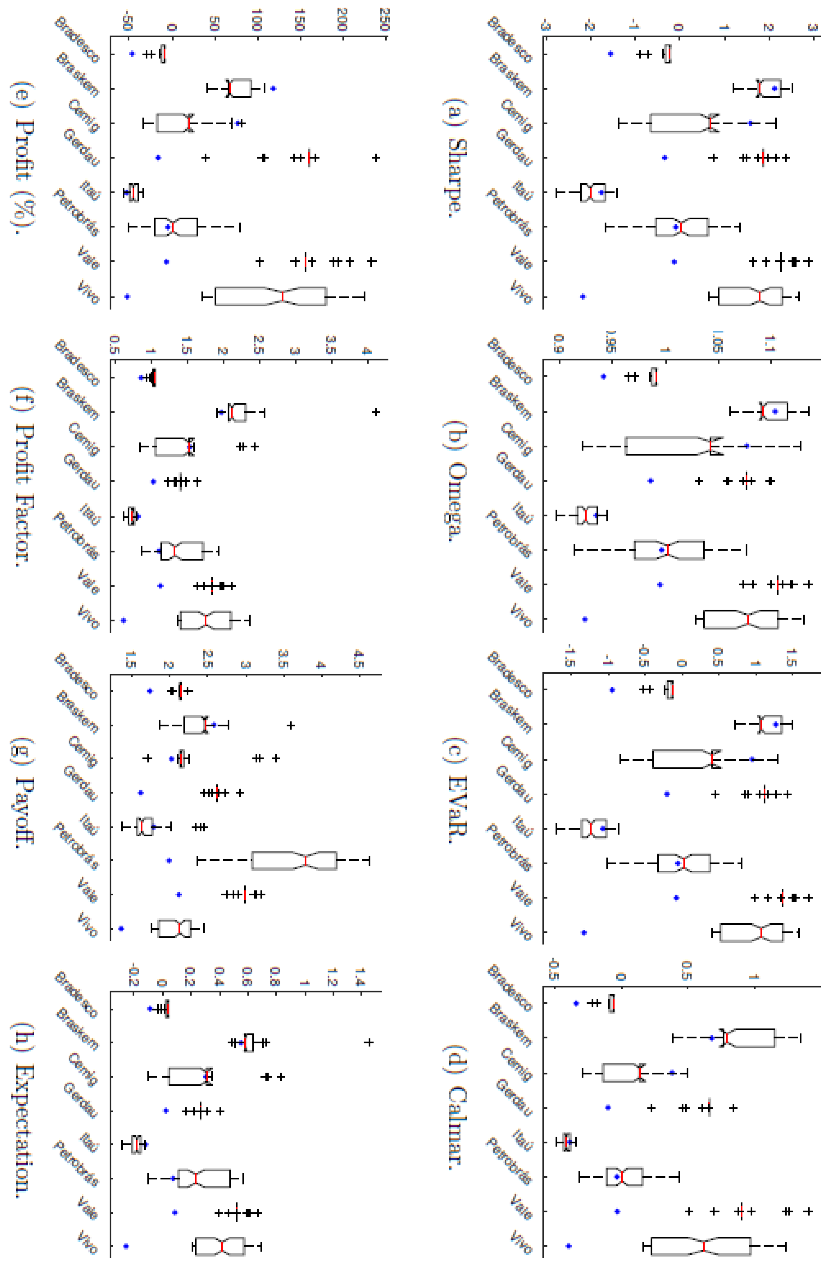
Regarding the weighting factor, interesting results appear. For all metrics, the results for GGBR4 and VALE3 present very small risk. The results tend toward a pronounced repeatability, except for a few outliers. On the one hand, for those securities, the entire distribution outperformed the ensemble TS. On the other hand, concerning risk, CMIG4 results present a superior statistical dispersion with a large distribution for Omega and a very small one for Payoff, for instance. Alternatively, the application of the proposed TS for PETR4 or VIVT4 tends to generate large distributions across all metrics. Even so, for VIVT4, the majority of the distribution was able to outperform the ensemble TS.
Another striking result is that it was always possible to combine a set of parameters such that the proposed TS outperformed the ensemble TS. The only exception occured for the combination of BRKM5 and Profit. In this case, the result of the ensemble TS fell above the top whisker. The analysis reveals that in many scenarios the central tendency of the proposed TS falls above the result produced by the ensemble TS. This is the case for security PETR4 for all the metrics analyzed.
The proposed approach can be regarded as less sensitive to variations in the mitigation factor. For instance, in comparison with the nominal experiment (θ = 0.5), there was a change in the selected TTR in only 10% of the scenarios. In Table 4 and Table 5 one can observe that the different values of θ did not result in striking modifications at the ranking order. As a conjecture, it may be pointed out that all the metrics, except Profit, already take risk factors into account. Since the mitigation factor is the same for all metrics, the effect of weighting more on the negative part of the S-curve becomes less relevant. In other words, it gives more weight to a factor that has already been penalized.
Figure 3 shows the dominance curve obtained empirically for the Sharpe Index. This is also consistent with the theory, with a noticeable S-shaped aspect reflecting the loss aversion principle (losses with the same level of gains have higher absolute value).
The proposed method shares the following advantages of the MCDA method class over other method classes: (i) it is more appealing to practitioners, as there is no single criterion to optimize within the constraints; (ii) it is easier and quicker to solve, as it does not require an optimization tool in general; (iii) it is easier to configure by changing weights and adding new criteria to the system; (iv) it incorporates prospect theory into the TS architecture, thereby providing a compromise solution between aspects of human decision-making and the objective decision-making process of the TTRs.

5. Conclusions

This article proposed a TS that adapts its strategy to the underlying data. In this algorithm, multiple TTRs are trained in parallel and evaluated against risk-adjusted and profitability-based performance metrics. Since several criteria are possible, a decision-making method based on prospect theory, TODIM, was employed to classify the TTRs, and the best placed was chosen as the trading strategy for a given period of time. Using the walk forward method, a new dataset fed TODIM TS with data for comparisons with B&H models and the comparison TS. Due to its methodology, as expected, TODIM TS obtained superior results according to the criteria aimed at analyzing risk. The experimental results suggest that the proposed ST has strong generalization and adaptability capabilities, providing improvements, or at least comparable results, in relation to an alternative ST based on a different decision-making method. The simple application, which can be used by beginner practitioners, and the low computational requirement for the analysis and selection of the TS also serve to differentiate the method. The results reinforce the suitability of a method based on prospect theory to select alternatives with lower risk, due to its greater aversion to the risk of loss.
In future work, the authors will seek to investigate an optimization method to select the parameters of the proposed decision-making process and consider improved TTRs. They will also propose to increase the study database so as to include more stocks for the comparison of methods.

Supplementary Materials

The following supporting information can be downloaded at: https://www.mdpi.com/article/10.3390/pr10030609/s1, Table S1: HML Factors, Table S2: IML Factors, Table S3: Market Factors, Table S4: Risk Free, Table S5: SMB Factors, Table S6: WML Factors.

Author Contributions

Conceptualization, B.P., M.L., L.M. and E.S.; methodology, B.P. and M.L.; software, M.L.; validation, L.M. and E.S.; formal analysis; investigation, E.S.; resources, B.P.; data curation, L.M. and M.L.; writing—original draft preparation, B.P., M.L., L.M. and E.S.; writing—review and editing, B.P.; visualization, L.M.; supervision, M.L.; project administration, E.S.; funding acquisition, E.S. All authors have read and agreed to the published version of the manuscript.

Funding

The authors would like to thank the Intel Center of Excellence in Artificial Intelligence at ITA for the funding support to complete this research work. This study was financed in part by the Coordenação de Aperfeiçoamento de Pessoal de Nível Superior–Brasil (CAPES) under grand no. 88887.634432/2021−00. This study was also funded in part by Fundação de Amparo à Pesquisa do estado de Minas Gerais (FAPEMIG) under the grant no. APQ−0091319. The Titan V used for this research was donated by the NVIDIA Corporation.

Institutional Review Board Statement

Not applicable.

Informed Consent Statement

Not applicable.

Data Availability Statement

The dataset were download from https://finance.yahoo.com (Accesed on 19 August 2020).

Conflicts of Interest

The authors declare no conflict of interest. The funders had no role in the design of the study; in the collection, analyses, or interpretation of data; in the writing of the manuscript, or in the decision to publish the results.

Appendix A. Data—Brazilian Stocks

The database used in this work is composed of a series of daily prices of some of the most prominent stocks in the main Brazilian stock market index (IBOVESPA), including: Bradesco, Itaú, Braskem, Cemig, Gerdau, Vivo, Petrobrás and Vale, respectively, with tickers BBDC4, ITUB4, BRKM5, CMIG4, GGBR4, VIVT4, PETR4 and VALE3. The analysis extended from 3 January 2002 to 31 December 2017. Figure A1 shows the capital curves. Table A1 presents the main statistics of the returns. These stocks were selected based on three different assumptions: (i) they were negotiated since 2 January 2000; (ii) they were from different economic sectors; and (iii) their particular weights to the IBOVESPA index were relevant. (This can be confirmed by the value of β. This parameter was calculated using the Fama–French three-factor model (Fama and French (1993)), in which the risk factors for Brazil were obtained on supplementary material in Tables S1–S6. The dataset was formed by daily closing prices and the period of analysis extended from 3 January 2002 to 31 December 2017.)
Figure A1. Capital cumulative curves of the securities used in this study.
Processes 10 00609 g0a1
Table A1. Statistics of the returns, N = 3961: Asymmetry (Asym.), Kurotsis (Kurt.), Jarque-Bera (JB) test. β is the Fama–French three-factor model (FF3) market beta, and S is the Sharpe ratio.
StockṜ (104)σ (10²)Asym.Kurt.JBβS (10²)
BBDC47.4312.2110.4738.09344290.513 *3.361
BRKM56.1402.7580.3216.65122670.353 *2.226
CMIG44.6912.539−0.2047.78838110.408 *1.848
GGBR46.0152.7610.2055.52010750.525 *2.179
ITUB47.0812.2680.6169.28767750.541 *3.122
PETR43.8322.6210.1466.64422050.595 *1.462
VALE37.1872.6160.1686.39719230.543 *2.747
VIVT45.3431.8230.1484.443358.20.238 *2.931
Note: * indicates p-value < 0.01.

Appendix B. Technical Indicators and Trading Rules Investigated

Figure A2 shows the classic TTRs selected for this work. Given the set of parameters in these tables, there is a total of 270 rules for each approach. Because the literature covering this topic is scattered, as well as for consistency purposes, we followed the implementation of [21]. For a description of trend-following rules and moving averages, as well as classic oscillators and Bollinger Bands, see the details in [21,38,39], respectively.
Figure A2. Technical trading rules based on classic indicators, classic-TTR.
Processes 10 00609 g0a2

Appendix C. Performance Metrics

In this paper, some performance metrics were adopted to evaluate the investment performance. Some measure profit, and others measure risk exposure.
The profit factor, F, is defined as the gross profit divided by the gross loss (sum of P winning trades S+ divided by Q losing trades S−). The payoff ratio, P, is the ratio of average win and average loss. The average is computed as the ratio between the geometric mean of winning P+ and of losing trades P−. The expected value is defined as the difference between expected profits and expected costs. These metrics are detailed in Figure A3.
Figure A3. Profit performance metrics.
Processes 10 00609 g0a3
One criticism of the aforementioned metrics is that the risk involved for obtaining the profit is not taken into account. If two or more investments have the same return over a given time period, the one that has the lowest risk is more likely to be selected. The prevailing approaches in the stock markets therefore include some risk metrics [40], called risk-adjusted metrics, which are computed according to:
R ¯ Υ R  
with γ standing for the risk-free interest rate (Rf), or target profit ζ; R is the geometrical mean of historical profit; and R can be several risk metrics. Without loss of generality, it is assumed that γ = 0.
The risk metrics, R, considered in this paper are shown in Figure A4. The Sharpe ratio, S, measures the return of the investment over the risk-free rate, also called the risk premium, compared to the total risk of the investment, measured by its standard deviation of returns, σr. A disadvantage is that downside and upside variability are penalized similarly. However, investors are more concerned with downward volatility.
Figure A4. Risk-adjusted performance metrics.
Processes 10 00609 g0a4
Another approach is to consider the lower partial moments, a downside risk metric Υ1(ζ) which measures risk by considering only those deviations that fall below an ex ante defined threshold, such as Omega Ω.
Another type of risk measure uses drawdowns, i.e., the peak-to-trough difference. The maximum drawdown of an asset denotes the maximum possible loss in a period. The Calmar Index, C, uses the maximum drawdown, MD1, as its risk measure. The issue here is to assess risk utilizing a single event, MD1.
Finally, the value at risk, ν, describes the possible loss of an investment, which is not exceeded by a given probability of 1 − α in a certain period [41]. The excess VaR, ϕ, is an example of this.

References

  1. Fama, E.F. Efficient capital markets: A review of theory and empirical work. J. Financ. 1970, 25, 383–417. [Google Scholar] [CrossRef]
  2. Franco, M.; Miller, M.H. The cost of capital, corporation finance and the theory of investment. American 1958, 1, 3. [Google Scholar]
  3. Harry, M. Portfolio selection. J. Financ. 1952, 7, 77–91. [Google Scholar]
  4. Fischer, B.; Jensen, M.C.; Scholes, M. The capital asset pricing model: Some empirical tests. Stud. Theory Cap. Mark. 1972, 81, 79–121. [Google Scholar]
  5. Fischer, B.; Scholes, M. The pricing of options and corporate liabilities. J. Polit. Econ. 1973, 81, 637–654. [Google Scholar]
  6. Lo Andrew, W. The Financial System Red in Tooth and Claw: 75 Years of Co-Evolving Markets and Technology. Financ. Anal. J. 2021, 77, 5–33. [Google Scholar]
  7. Daniel, K.; Tversky, A. Prospect Theory: An Analysis of Decision under Risk. Econometrica 1979, 47, 263–291. [Google Scholar]
  8. Amos, T.; Kahneman, D. Advances in prospect theory: Cumulative representation of uncertainty. J. Risk Uncertain. 1992, 5, 297–323. [Google Scholar]
  9. Hersh, S.; Statman, M. Behavioral capital asset pricing theory. J. Financ. Quant. Anal. 1994, 29, 323–349. [Google Scholar]
  10. Nicholas, B.; Thaler, R. A survey of behavioral finance. Handb. Econ. Financ. 2003, 1, 1053–1128. [Google Scholar]
  11. Andreu, M.; Whinston, M.D.; Green, J.R. Microeconomic Theory; Oxford University Press: New York, NY, USA, 1995; Volume 1. [Google Scholar]
  12. David, L.; Zeckhauser, R. Amos Tversky and the ascent of behavioral economics. J. Risk Uncertain. 1998, 16, 7–47. [Google Scholar]
  13. Shiller, R.J. From efficient markets theory to behavioral finance. J. Econ. Perspect. 2003, 17, 83–104. [Google Scholar] [CrossRef] [Green Version]
  14. Thaler, R.H. Misbehaving: The Making of Behavioral Economics; Norton: New York, NY, USA, 2015. [Google Scholar]
  15. David, B.; Cannon, E.; Wright, D. Quantifying loss aversion: Evidence from a UK population survey. J. Risk Uncertain. 2021, 63, 27–57. [Google Scholar]
  16. Junbo, W.; Wu, C.; Zhong, X. Prospect theory and stock returns: Evidence from foreign share markets. Pac.-Basin Financ. J. 2021, 69, 101644. [Google Scholar]
  17. Nicholas, B.; Mukherjee, A.; Wang, B. Prospect Theory and Stock Returns: An Empirical Test. Rev. Financ. Stud. 2016, 29, 3068–3107. [Google Scholar]
  18. Joãoo, N.A.; Klotzle, M.C.; Brandão, L.E.T.; Pinto, A.C.F. Prospect theory and narrow framing bias: Evidence from emerging markets. Q. Rev. Econ. Financ. 2021, 80, 90–101. [Google Scholar]
  19. Farias, N.R.T.; Silva, J.L.; Sobreiro, V.A.; Kimura, H. A Literature Review of Technical Analysis on Stock Markets. Q. Rev. Econ. Financ. 2017, 66, 115–126. [Google Scholar] [CrossRef]
  20. Daniel, G. Systematic investment strategies. Financ. Anal. J. 2017, 73, 10–14. [Google Scholar]
  21. Leles, M.C.R.; Mozelli, L.A.; Sbruzzi, E.F.; Júnior, C.L.N.; Guimarães, H.N. A multicriteria trading system based on singular spectrum analysis trading rules. IEEE Syst. J. 2019, 14, 1468–1478. [Google Scholar] [CrossRef]
  22. Cavalcante, R.C.; Brasileiro, R.C.; Souza, V.L.F.; Nobrega, J.P.; Oliveira, A.L.I. Computational intelligence and financial markets: A survey and future directions. Expert Syst. Appl. 2016, 55, 194–211. [Google Scholar] [CrossRef]
  23. Christian, R.K.; Jones, R.C. Machine Learning for Stock Selection. Financ. Anal. J. 2019, 75, 70–88. [Google Scholar]
  24. Lennart, O.; Waack, S. Demonstrating non-inferiority of easy interpretable methods for insolvency prediction. Expert Syst. Appl. 2015, 42, 9117–9128, ISSN 0957-4174. [Google Scholar]
  25. Gomes, L.; Lima, M. TODIM: Basics and application to multicriteria ranking of projects with environmental impacts. Found. Comput. Decis. Sci. 1991, 16, 113–127. [Google Scholar]
  26. Michael, D.; Zopounidis, C. Multicriteria Decision Aid Classification Methods; Springer Science & Business Media: Berlin/Heidelberg, Germany, 2002; Volume 73. [Google Scholar]
  27. Barba-Romero, S.; Pomerol, J.C. Decisiones multicriterio: Fundamentos teoricos y utilizacion practica. In Coleccion de Economia; Universidad de Alcala: Alcala de Henares, Spain, 1997. [Google Scholar]
  28. Jaap, S.; Steuer, R.E.; Zopounidis, C. Multicriteria decision aid/analysis in finance. In Multiple Criteria Decision Analysis; Springer: Amsterdam, The Netherlands, 2016; pp. 1011–1065. [Google Scholar]
  29. Fatih, A.; Tolga, A.C. Portfolio allocation with the TODIM method. Expert Syst. Appl. 2019, 124, 341–348. [Google Scholar]
  30. Lima, C.P.A.; Teodoro, A.R.B.; de Castro, L.I.; Parsons, S. Expected utility or prospect theory: Which better fits agent based modeling of markets? J. Comput. Sci. 2016, 17, 97–102. [Google Scholar]
  31. Magalhães, R.F.; Rangel, L.A.D.; Sbruzzi, E.F.; Nascimento, C.L.; Leles, M.C.R. Analysis of the Brazilian Research Agencies using a Multicriteria Decision Aid known as TODIM. In Proceedings of the 2019 IEEE International Systems Conference (SysCon), Orlando, FL, USA, 1–6 April 2019. [Google Scholar]
  32. Jean-Pierre, B.; Vincke, P. A Preference Ranking Organisation Method: (The PROMETHEE Method for Multiple Criteria Decision-Making). Manag. Sci. 1985, 31, 647–656. [Google Scholar]
  33. Peijia, R.; Xu, Z.; Gou, X. Pythagorean fuzzy TODIM approach to multi-criteria decision making. Appl. Soft Comput. 2016, 42, 246–259. [Google Scholar]
  34. Gomes, L.; Rangel, L. An application of the TODIM method to the multicriteria rental evaluation of residential properties. Eur. J. Oper. Res. 2009, 193, 204–211. [Google Scholar] [CrossRef]
  35. Rodolfo, L.; Krohling, R.A. The Hellinger distance in Multicriteria Decision Making: An illustration to the TOPSIS and TODIM methods. Expert Syst. Appl. 2014, 41, 4414–4421. [Google Scholar]
  36. López, P.M. Advances in Financial Machine Learning; John Wiley & Sons: Hoboken, NJ, USA, 2018. [Google Scholar]
  37. Massoud, M.; Chen, C.H.; Hayes, L.A. History of share prices and market efficiency of the Madrid general stock index. Int. Rev. Financ. Anal. 2015, 40, 178–184. [Google Scholar]
  38. Leles, M.C.R.; Mozelli, L.A.; Guimarães, H.N. New Trend-Following Indicator: Using SSA to Design Trading Rules. Fluct. Noise Lett. 2017, 2, 1750016. [Google Scholar] [CrossRef]
  39. Leles, M.C.R.; Mozelli, L.A.; Nascimento-Junior, C.L.; Sbruzzi, E.F.; Guimarães, H.N. Study on Singular Spectrum Analysis as a New Technical Oscillator for Trading Rules Design. Fluct. Noise Lett. 2018, 17, 1850034. [Google Scholar] [CrossRef]
  40. Robert, P. The Evaluation and Optimization of Trading Strategies; John Wiley & Sons: Hoboken, NJ, USA, 2011; Volume 314. [Google Scholar]
  41. Carol, A. Market Risk Analysis, Value at Risk Models; John Wiley & Sons: Hoboken, NJ, USA, 2009; Volume 4. [Google Scholar]
Figure 1. S-shaped curve of prospect theory. Diminishing sensitivity: as wealth grows, the impact of a given increment of wealth falls. Loss aversion: individuals respond asymmetrically to gain and losses.
Processes 10 00609 g001
Figure 2. Details of the proposed approach compared with the methodology used in [21] for a multicriteria trading system design. (a) Trading system simulation based on the walk forward method. (b) Optimization process detailed. Comparison of ensemble method [21] and the proposed approach. Although the two methods are based on the same matrix, the two multicriteria approaches might choose different TTRs at each iteration. (c) Capital curves depicting one of the simulations: the time series under analysis (black color) and two methodologies for the trading system development discussed. TODIM refers to the proposed approach, while ENSEMBLE indicates the method of [21].
Processes 10 00609 g002
Figure 3. Empirical S-shaped curve for the Sharpe Index. Similar results were found for other performance metrics but are omitted due to space restrictions.
Processes 10 00609 g003
Figure 4. Distribution of results according to changes in the weighting factors. The blue cross indicates the ensemble outcomes.
Processes 10 00609 g004
Table 1. Statistics of difference between the average return for a trading system (TS) and the buy and hold (B&H). (By the authors.)
TickMethod2007–20102011–20142015–20172007–2017
t-Statp-Valuet-Statp-Valuet-Statp-Valuet-Statp-Value
BBDC4TOD−1.4030.161−1.3010.193−0.4630.644−1.9010.057
ENS−1.7580.079−1.3310.184−1.2330.218−2.5260.012
BRKM5TOD−0.4640.6430.4840.628−1.6850.092−0.9230.356
ENS−0.5490.583−0.4280.669−0.9670.334−1.1020.271
CMIG4TOD−1.4320.1530.0210.983−0.0110.991−0.7750.438
ENS−1.6000.110−0.1870.8520.6590.510−0.3860.699
GGBR4TOD−1.2180.2230.1600.8730.1900.850−0.6750.500
ENS−0.5290.5970.9980.319−1.2810.201−0.5680.570
ITUB4TOD−0.8510.395−0.6040.546−0.6110.541−1.1670.243
ENS−1.5900.112−1.3650.173−1.8260.068−2.6490.008
PETR4TOD0.2140.8300.8200.412−0.7020.4830.2350.815
ENS−0.4840.6290.3030.762−0.7040.482−0.4750.635
VALE3TOD−0.1370.8910.7390.460−0.9790.328−0.4270.670
ENS−1.0350.301−0.4270.669−0.4590.646−1.1900.234
VIVT4TOD−0.9970.319−1.2310.218−1.9420.052−2.1950.028
ENS−1.7300.084−2.2800.023−0.8340.404−2.8070.005
Table 2. Risk metrics. (By the authors.)
TickYearStd.Dev. (%)LPM (10³)Max.DD. (%)VaR (10²)
TODB&HENSTODB&HENSTODB&HENSTODB&HENS
BBDC42007–20101.622.611.724.518.855.1254.8952.4461.662.644.362.79
2011–20141.181.851.163.066.662.7834.8026.0931.151.933.101.89
2015–20171.562.141.503.347.413.7826.5844.3335.512.643.612.49
2007–20171.462.231.483.677.663.9154.8952.4467.772.403.732.41
BRKM52007–20102.002.911.534.8710.023.4753.2975.7642.443.334.872.56
2011–20141.582.311.053.868.432.3830.4756.2141.772.653.831.73
2015–20172.102.821.465.299.002.4231.3640.5523.223.534.832.51
2007–20171.892.681.364.629.162.7853.2975.7642.443.164.502.27
CMIG42007–20100.732.181.341.077.773.0341.5534.6755.221.173.642.18
2011–20140.962.081.341.557.023.2711.8243.2230.461.653.492.27
2015–20171.283.251.292.2812.031.6339.4072.1821.972.125.342.20
2007–20170.992.481.331.578.662.7447.9875.3755.221.644.132.22
GGBR42007–20101.133.132.162.0111.185.5934.7174.5055.551.835.233.60
2011–20140.912.161.161.928.562.7253.0564.7324.951.463.501.91
2015–20172.443.422.235.1812.475.6044.2470.0345.454.145.733.65
2007–20171.552.911.882.8410.594.5575.8890.9064.502.554.823.11
ITUB42007–20100.922.872.051.409.376.0818.0056.3665.611.534.813.36
2011–20140.701.881.071.326.952.8820.4836.2745.861.153.121.73
2015–20171.521.991.443.906.733.6818.3633.5531.832.573.372.37
2007–20171.062.311.582.057.774.2623.4456.3672.111.763.872.59
PETR42007–20101.592.751.784.119.444.4226.0167.8345.182.694.582.96
2011–20140.832.481.471.189.273.8018.6162.8744.621.384.032.38
2015–20172.073.432.354.9911.936.1331.6570.7944.603.475.783.93
2007–20171.532.861.853.2810.084.6638.4789.5754.052.564.753.06
VALE32007–20101.743.021.864.3010.214.9523.9868.5260.382.955.073.09
2011–20141.211.911.103.367.603.0534.9761.3459.001.983.091.73
2015–20172.173.522.664.1712.586.5735.1967.5853.053.635.964.50
2007–20171.712.831.913.929.914.7149.6082.9383.322.854.723.15
VIVT42007–20100.921.941.342.277.033.7738.4337.0356.791.493.222.16
2011–20141.241.581.213.425.693.5923.1422.6238.042.072.661.97
2015–20171.101.601.172.895.793.2042.2638.4132.221.782.681.93
2007–20171.101.721.252.876.213.5546.3238.4168.641.792.882.03
Table 3. Performance metrics: risk-adjusted. (By the authors.) The results in which the performance of the TOD model is superior to that of the ENS are highlighted.
TickYearSharpeOmegaE. VAR (10²)Calmar (10²)
TODENSTODENSTODENSTODENS
BBDC42007–2010−1.834−2.8800.9340.903−1.122−1.773−0.540−0.803
2011–2014−1.664−1.8460.9360.923−1.018−1.131−0.565−0.688
2015–20173.5260.7861.1651.0312.0890.4742.0740.332
2007–2017−0.225−1.5540.9910.941−0.136−0.950−0.060−0.338
BRKM52007–20101.2541.3771.0521.0610.7520.8270.4710.498
2011–20142.360−0.9201.0970.9591.408−0.5611.225−0.232
2015–20172.2596.1791.0901.3741.3463.6051.5143.895
2007–20171.8662.1191.0761.1031.1151.2670.6610.677
CMIG42007–2010−5.685−3.1110.6110.862−3.571−1.920−1.002−0.757
2011–20147.1693.9831.4441.1634.1652.3555.8041.754
2015–2017−0.9284.7440.9471.376−0.5652.793−0.3042.796
2007–20170.6671.5791.0421.0770.4030.9470.1380.380
GGBR42007–2010−3.4600.8750.8051.034−2.1410.526−1.1270.341
2011–2014−5.757−0.6200.7260.974−3.617−0.377−0.992−0.288
2015–20173.761−1.8821.1770.9252.219−1.1492.077−0.922
2007–2017−0.540−0.3420.9710.986−0.328−0.207−0.110−0.100
ITUB42007–20100.974−1.7371.0640.9410.587−1.0610.500−0.543
2011–20140.059−3.3821.0030.8740.036−2.0920.020−0.791
2015–20173.676−0.4401.1430.9832.176−0.2673.045−0.199
2007–20171.763−1.7591.0910.9351.057−1.0760.795−0.386
PETR42007–20103.9100.6351.1511.0262.3110.3822.3900.250
2011–20140.536−3.0361.0380.8830.324−1.8720.240−0.997
2015–20171.9091.6761.0791.0641.1401.0021.2510.883
2007–20172.260−0.0961.1050.9961.349−0.0580.898−0.033
VALE32007–20104.7370.6691.1921.0252.7850.4033.4300.207
2011–2014−2.215−7.4250.9200.733−1.360−4.711−0.770−1.384
2015–20171.7663.2881.0921.1331.0551.9451.0881.650
2007–20171.785−0.1301.0780.9951.068−0.0780.614−0.030
VIVT42007–2010−2.914−4.0820.8820.855−1.798−2.534−0.699−0.962
2011–20141.204−1.6871.0440.9430.724−1.0320.648−0.535
2015–2017−4.0150.3470.8471.013−2.4930.210−1.0480.126
2007–2017−1.564−2.1730.9400.924−0.956−1.334−0.371−0.395
Table 4. Performance metrics: profit-based. (By the authors.) The results in which the performance of the TOD model is superior to that of the ENS are highlighted.
TickYearProfit (%)Payoff P. FactorExpect.
TODENSTODENSTODENSTODENS
BBDC42007–2010−25.36−38.630.8990.7102.3721.584−0.073−0.200
2011–2014−17.69−19.110.7870.6581.1811.317−0.128−0.228
2015–201750.379.115.5361.1571.8452.1211.1340.102
2007–2017−8.53−46.381.0590.8682.1421.7360.039−0.088
BRKM52007–201028.0723.151.3161.4242.7421.7470.2140.233
2011–201444.72−9.151.4050.7762.2731.9400.250−0.160
2015–201742.0795.241.57710.2103.39610.2100.3944.605
2007–2017160.40118.431.4101.9752.6212.5820.2670.552
CMIG42007–2010−33.67−33.800.2620.5821.0501.979−0.590−0.323
2011–201497.2169.6812.8791.9724.2932.0362.9700.494
2015–2017−8.4957.511.03315.0492.0667.5240.0224.683
2007–201719.7176.931.5281.5372.1402.0220.3080.305
GGBR42007–2010−32.0020.52NaN1.228NaN1.661NaN0.131
2011–2014−40.63−6.880.4150.9302.0751.438−0.488−0.042
2015–201797.33−26.674.5600.5834.5601.5821.780−0.305
2007–2017−20.33−16.031.1431.0374.1911.6150.1120.022
ITUB42007–20109.28−29.631.3100.9131.8341.5220.181−0.054
2011–20140.41−30.181.0820.5691.0821.3820.041−0.305
2015–201751.21−4.5911.0431.0065.5212.4153.3480.004
2007–201765.93−53.122.0720.8252.4601.7870.582−0.120
PETR42007–201084.5611.801.8641.1882.5301.7820.4980.113
2011–20144.52−35.631.7200.4191.7201.6750.360−0.465
2015–201734.0433.801.8221.6634.5542.4950.5870.398
2007–2017155.81−4.731.8421.1152.9941.9870.5210.074
VALE32007–2010124.9713.083.5911.2563.0381.8481.1870.153
2011–2014−23.39−55.450.7450.3931.3041.153−0.162−0.453
2015–201732.7491.102.2581.7851.6932.5500.5390.462
2007–2017128.77−6.501.7651.1332.1312.1170.4190.087
VIVT42007–2010−23.27−41.660.2000.3910.3341.123−0.500−0.452
2011–201415.99−18.271.3600.6232.7201.5580.240−0.269
2015–2017−27.943.040.6651.1501.6081.495−0.2370.085
2007–2017−37.29−52.110.8010.6241.6871.357−0.135−0.258
Table 5. Sensibility analysis for the first 10 TTR (technical trading rules) indexes ranked via TODIM. (By the authors.)
θ1st2nd3rd4th5th6th7th8th9th10th
0.155495247616467703136
0.25554952476164677032
0.55549526747616470358
0.755549675247646158703
0.95549675247586470613
Table 6. Sensibility analysis for the chosen TTR at each iteration. (By the authors.)
θ20072008200920102011201220132014201520162017
0.155914414568203202203218155
0.2555914414568203202203218155
0.555914414568203202218218155
0.7555914414568203202218182155
0.955914414568175202218182155
Publisher’s Note: MDPI stays neutral with regard to jurisdictional claims in published maps and institutional affiliations.

