1. Introduction
The effects of global climate change can be observed and felt particularly strongly in cities. The idea of reducing the solar overheating of urban surfaces has become more and more widespread, especially in recent years, during discussions about the urban heat island (UHI) effect [
1]. One measure to reduce or eliminate these urban heat islands are greening measures, as well as water areas (artificial lakes, fountains, etc.) [
2,
3]. However, the use of these solutions is not always sufficient or approvable, or desirable, e.g., for old buildings, and historical or listed buildings.
Many recent studies have focused on the geothermal potential of UHIs. Bayer et al. [
4] reviewed the capacity of shallow geothermal energy in cities. Zhu et al. [
5] studied geothermal potential due to the elevated temperatures of aquifers as thermal energy reservoirs, especially in Cologne (Germany) and Winnipeg (Canada).
Thus far, little attention has been paid to the “harvesting” of solar urban excess heat from building surfaces, sidewalks, roads, and squares through shallow absorber ducts, which are then used in borehole heat exchanger (BHE) fields as thermal energy storage (TES) systems for later use as heat sources for buildings. However, since the temperatures of urban surfaces are sometimes very high and these cannot easily be introduced into BHE fields, common calculations and simulations are not sufficient to accurately predict the thermal behavior of subsoil in densely built sensitive urban spaces with a lot of area competition.
The thermal behavior of a BHE field strongly depends on the thermal properties of the used ground, as shown by Gultekin et al. [
6]. In the study of Dalla Santa et al. [
7], the importance of the thermal properties of a subsurface in the design and configuration of a BHE, especially for ground source heat pump (GSHP) applications, is emphasized. The researchers reported that an overestimated ground thermal conductivity would lead to an undersized heat exchange area and a lower energy efficiency of the system, and an underestimated ground thermal conductivity would lead to higher initial costs. Therefore, accurate knowledge of the effective thermal conductivity is crucial for the optimal design of a BHE in a GSHP application. In the case of soil-based TES systems, the specific heat capacity of surrounding soil is needed to calculate the actual amount of heat stored per volume, as shown by Jradi et al. [
8].
In this work, we measure these thermal properties directly from extracted drill cores from different depths, and at different temperatures, from a BHE in Vienna. A detailed sample description is given at the beginning of the next section. The temperature-dependent effective thermal conductivity and the temperature-dependent specific heat capacity in a moist and dry state were determined by means of a heat flow meter (HFM) and differential scanning calorimetry (DSC).
In the study of Dalla Santa et al. [
7], four thermal conductivity measurement techniques were applied to measure the effective thermal conductivity of sedimentary rocks, igneous rocks, metamorphic rocks, and unconsolidated sediments. The only stationary method used was a modified guarded hot plate (GHP) system, which was only applied to gravel. In this study, we used a commercial HFM system without modifications to directly investigate the applicability of the process on drill core segments. New sample preparation routines were applied to determine the effective thermal conductivity of the moist, as well as the dry, state for different drill core sections and at different temperature points.
In the work of Abu-Hamdeh [
9], the influence of the soil density and water content on the thermal properties was shown. In the study, the author measured heat capacity based on the calorimetric method published in [
10], where the soil sample was heated in a capsule of copper with an internal thermocouple, but without information about the uncertainty of the device and the shown heat capacity results. In the publication of Wang et al. [
11], the standardized DSC method for specific heat measurements of soil solids was applied at room temperature. Our work also used the DSC method for the determination of the specific heat capacity, focusing directly on a broader temperature range and on sample preparation from the drill core segments in the actual moist and dry states.
Finally, we also investigated the thermal expansion of the different drill core segments to understand the expansion behavior of the subsurface in current wet and dry conditions at the expected temperatures.
2. Materials and Methods
2.1. Subsoil and Drill Core
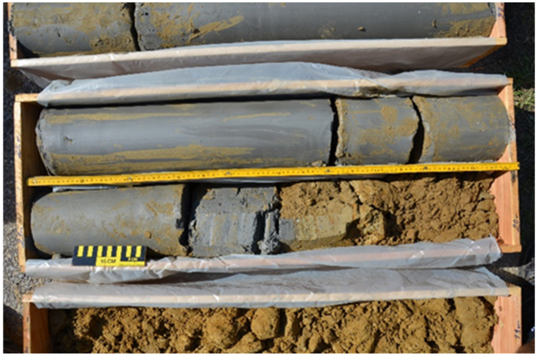
A large geophysical test field was built at the site of the Geological Survey of Austria. Part of the test field is a BHE, which was core-drilled to a depth of 80 m. As a result, the drill core (
Figure 1) was available for detailed investigations, which included, amongst others, mineralogy, geochemistry, thermal conductivity, heat capacity, and soil moisture.
The borehole heat exchanger consisted of a double-U tube with fiber-optic hybrid measurement cables for temperature measurements along the tubes. The fiber-optic temperature measurement made it possible to determine the temperature with a high resolution and high precision over the entire length of the borehole during the experiments. In addition to the glass fiber strands, a heating cable was also installed in the hybrid cables. This heating cable could also be used to directly heat the subsurface for experiments, with which more detailed information about the layer structure and the thermal and hydrological behavior of the subsurface could be obtained.
The measurement data provided important information about the heat flows that take place inside, and around, the BHE. The fiber optic temperature measurements were in the case of thermal response tests, such as those carried out for conventional geothermal probes, and only the fluid temperatures of the flow and return could be measured at the probe head. In addition, three observation probes were built around the geothermal probe and were fitted with fiber-optic measuring cables in order to investigate heat propagation during long-term experiments. Both aspects, the heat flows inside the probe as well as the heat conduction and heat storage behavior of the subsurface, were of high relevance for the question at hand.
2.2. Determination of the Specific Heat Capacity
The enthalpy of a substance increases with increasing temperature. It can be described as enthalpy change
, which is defined by the product of temperature difference
and heat capacity at constant pressure
of the material, as long as the heat capacity is constant over the range of temperatures of interest. The specific heat capacity at constant pressure
is defined as heat capacity related to mass. The temperature dependency of specific heat capacity
becomes more important for larger temperature differences.
The heat capacity of a material is specified through the substance type, mass, and the temperature itself.
2.2.1. Differential Scanning Calorimetry—DSC
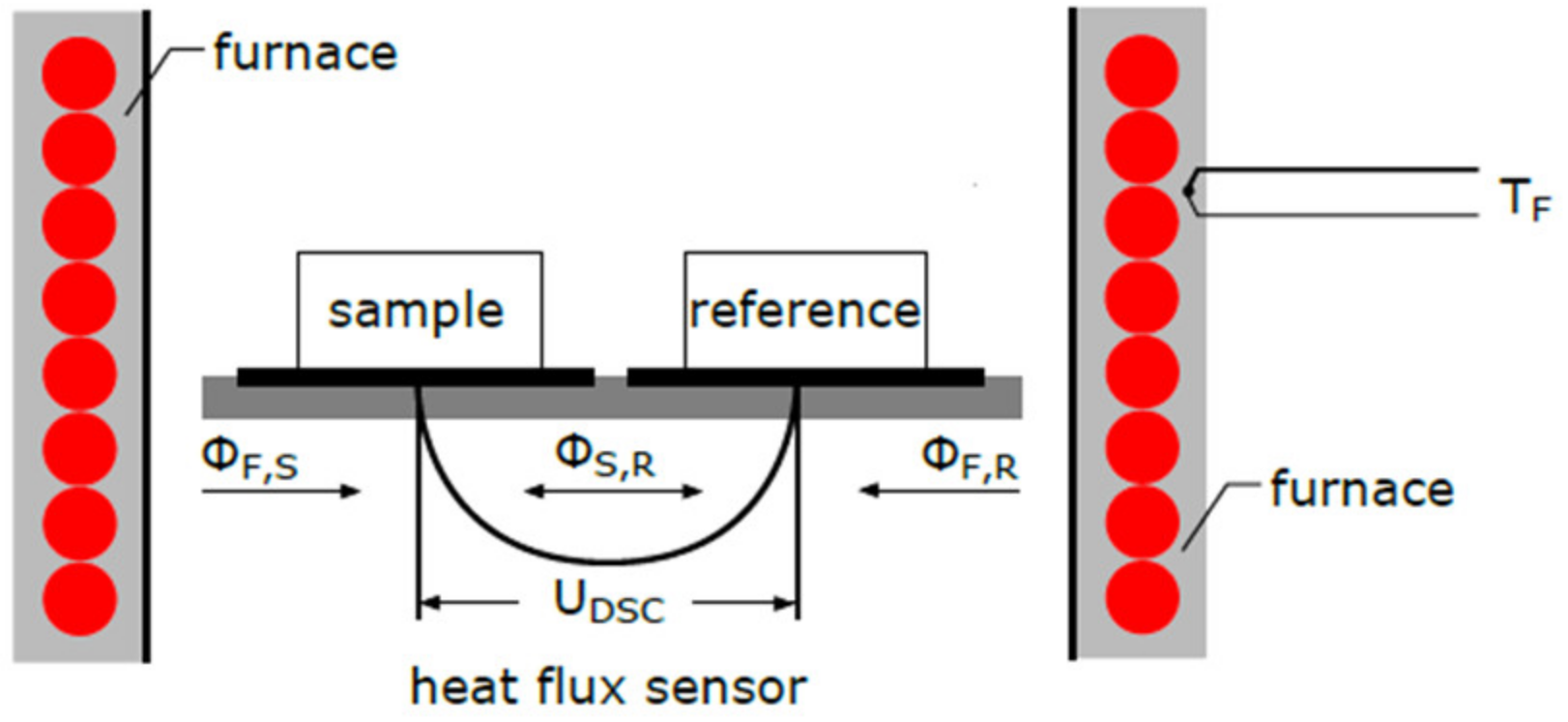
The main purpose of a calorimeter is to measure the exchange of heat. In this work, a 204 F1 DSC disc-type heat flux DSC (s.
Figure 2) from NETZSCH was used for the determination of the specific heat capacity.
Specific heat capacity
is the amount of heat required to raise the temperature of a substance by 1 K at a constant pressure without a first-order phase transition. According to the German Institute for Standardization (DIN) 51007 standard [
12], at least three measurement runs are needed to evaluate the
of a substance: a zero-line measurement with empty crucibles, a standard reference measurement (e.g., α-Al
2O
3 sapphire standard), and a sample measurement.
Following equation describes the determination of the specific heat capacity of a sample,
, by the product of the specific heat of the reference material,
the ratio of the reference mass,
, and sample mass,
, and the ratio of the zero line corrected measured DSC voltage of the sample,
, and the reference,
.
2.2.2. Sample Preparation
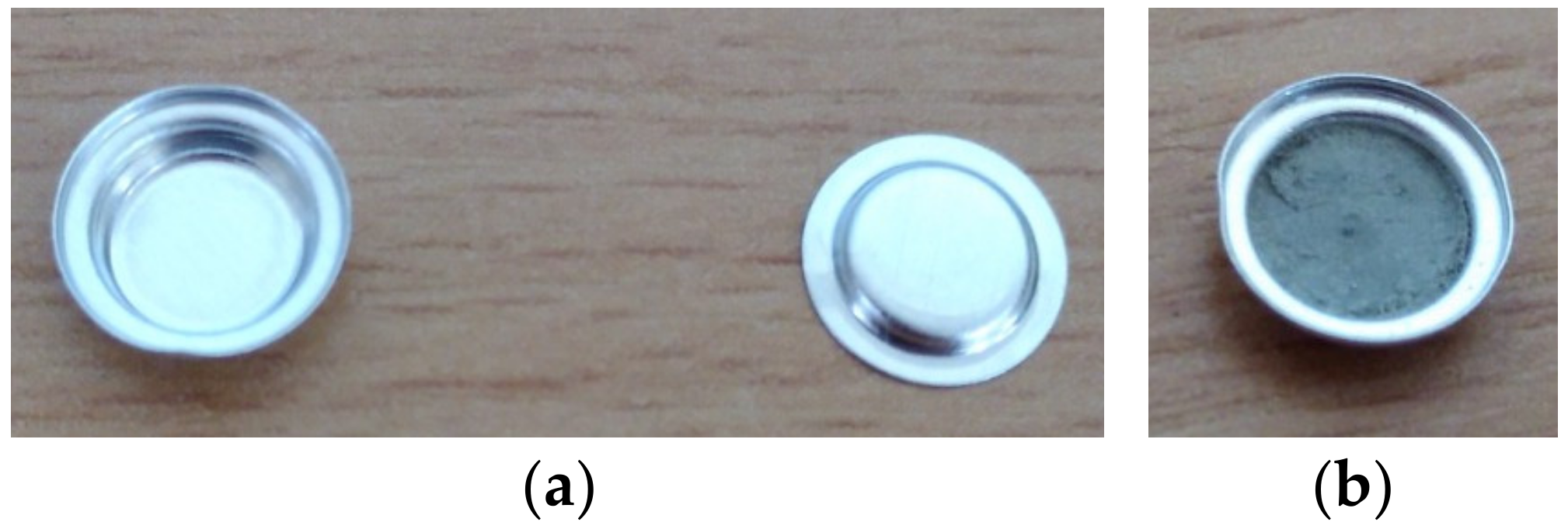
The samples for DSC measurements were prepared directly from the moist drill core samples or the dried HFM samples after the lab furnace drying procedure, which is described in the HFM sample preparation section. At least three samples per depth were measured for the DSC. For the experiment, aluminum crucibles with a volume of
were used and filled with sample (s.
Figure 3). Afterwards, the crucibles were closed and cold welded with an aluminum lid. The used sample masses were between
m =
for the moist and dry samples.
2.2.3. Measurement Procedure
All DSC experiments were conducted under dynamic He gas conditions with a gas flow of . The temperature program of the DSC furnace was defined as follows:
Start at 25 °C;
Cooling segment to −30 °C with 10 K min−1;
Isotherm segment at −30 °C for 5 min;
Heating segment to 60 °C with 20 K min−1.
Before every sample set consisting of three samples for each depth, three zero-line measurements with empty crucibles were measured. Thereafter, the three sample measurements for the current drill core depth followed by three sapphire-reference standard measurements were conducted. This procedure was repeated 4 times for the moist samples and 4 times for the dry samples. In total, 72 DSC measurements were executed for the evaluation of the specific heat capacity of the subsoil samples.
2.2.4. Evaluation and Uncertainty
As described in
Section 2.2.1, specific heat capacity was evaluated by the product of the specific heat capacity of the reference material, the ratio of the reference and sample mass, and the ratio of the zero-line corrected measured DSC voltage of the sample and the reference. The results shown in the evaluation are the mean values of three individual measurements.
Additionally, the represented uncertainty is calculated according the “Guide to the expression of uncertainty in measurement” [
13]. The expanded combined standard uncertainty is expressed with uncorrelated input quantities and a coverage factor of k = 2 (95% confidence interval) based on the input function from Equation (2).
2.3. Determination of the Thermal Conductivity
The thermal conductivity of the subsoil at different depths can help to determine the actual heat flux between the geothermal probe and its surroundings. This valuable input can be delivered by steady state and dynamic thermal conductivity measurement methods. In this work, a steady state method, also known as the heat flow meter (HFM), will be described.
In the simplified case of one-dimensional heat conduction in a solid body with two parallel wall areas, it is described through Fourier’s law, as shown in following equation:
where
corresponds to the heat flux density,
is the heat flux,
is the cross-sectional area,
is the thermal conductivity and
is the observed layer thickness. More information about the theory of thermal conductivity can be found in [
14]. An extensive summary of available steady state and dynamic thermal conductivity measurement methods are shown in [
15].
2.3.1. Heat Flow Meter—HFM
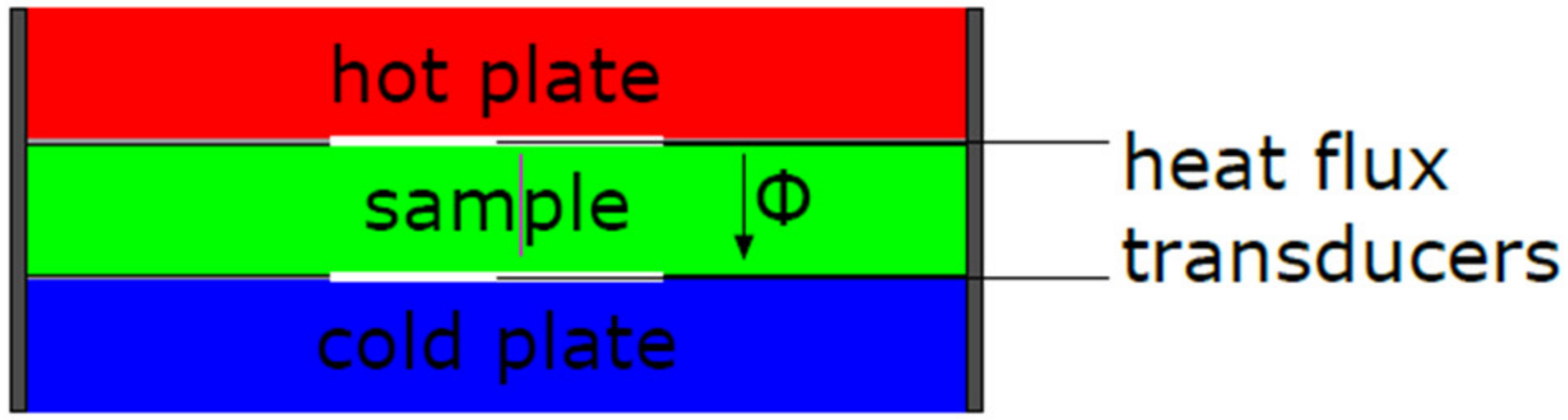
The HFM technique is a steady-state method to measure thermal conductivity
of solid materials by applying defined temperature difference
across the sample and measure heat flow
over a defined area, resulting in heat flux density
(s.
Figure 4).
For accurate results of constant one-directional heat flow
, it is necessary to have plane-parallel, homogeneous samples between the plates. To measure materials with high thermal conductivity,
, it is recommended [
16] to prepare thicker samples to increase the overall thermal resistance,
. Additionally, it has been stated that the influence of thermal contact resistance
between the plates and the sample increases with a low
of the sample.
In this work a NETZSCH HFM 446 Lambda Medium (NETZSCH-Gerätebau GmbH, Selb, Germany) device was used and the specifications are listed in
Table 1.
In case of the investigated drill core samples, an applied NETZSCH HFM 446 Lambda Medium device was equipped with a special instrumentation kit that was used to increase the of the sample setup. The equipment manufacturer defines a threshold of to apply the instrumentation kit consisting of interface pads made from compressible rubber as well as additional thermocouples.
2.3.2. Sample Preparation
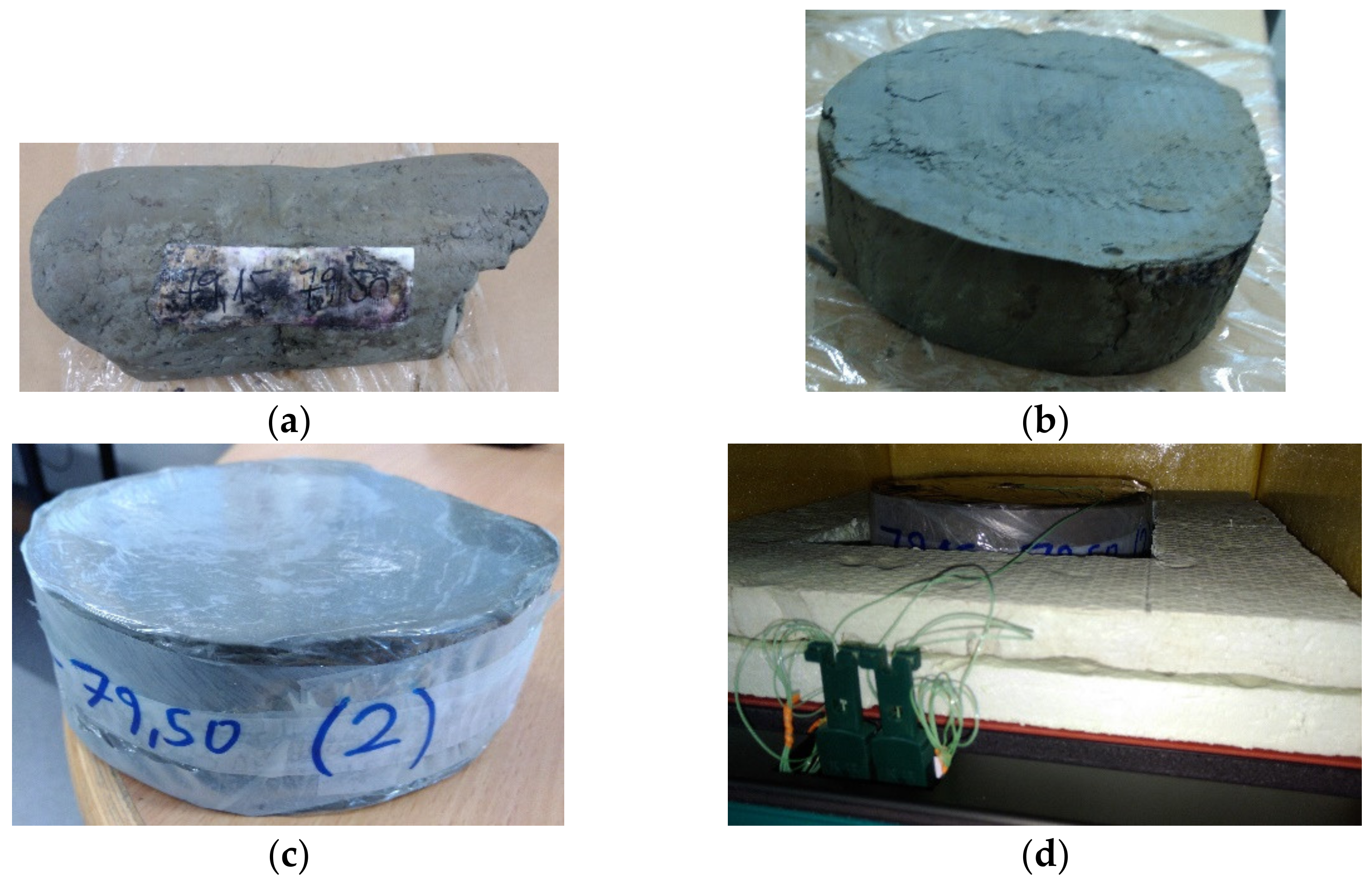
Figure 5 shows sample preparation for HFM samples, starting from parts of the available drill core to the final setup in the HFM measurement device.
Slices with a thickness of approx. 5 cm were cut from different parts of the drill core. The circular surfaces were scraped with a knife to acquire a homogenous thickness for the whole sample. After that, the sample was packed into polyethylene foil to avoid further drying of the drill core sample during the experiment, and additional thermocouples (Type K) were stuck to the center of the two circular surfaces. Finally, the sample with two thermocouples was placed in the HFM between two rubber sheets, for better contact conditions, between the heat flux plates and the sample, and with a surrounding polystyrene insulation to minimize lateral heat fluxes.
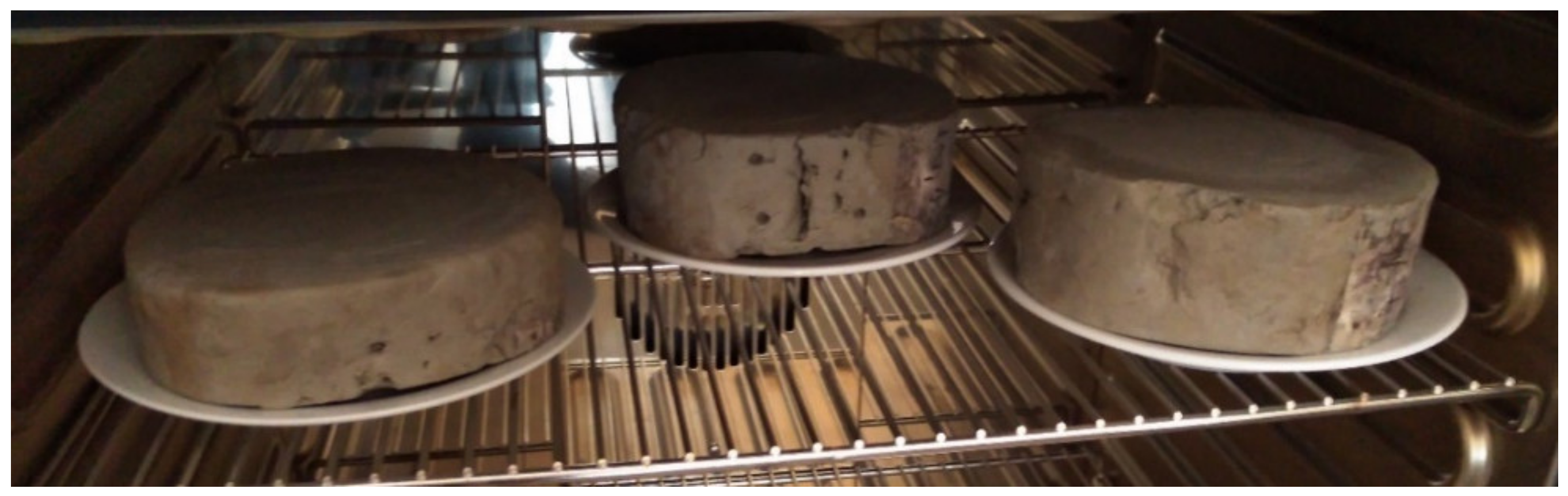
After the HFM measurements of the moist drill core samples, the samples were dried in a lab furnace at T = 105 °C (
Figure 6). The duration of the drying process depended on the moisture content of the sample and was checked regularly with a lab balance until no mass changes were detected.
After the drying process, samples were put into the HFM system, as shown in
Figure 5d, without any Polyethylen (PE) foil. The thermocouples were stuck in the center of the two circular surfaces on the top and bottom of the samples.
The thickness of the samples was measured in several places using a Mitutoyo CD-15CPX (Mitutoyo Corporation, Sakado, Japan) caliper and the weight was determined using a Sartorius TE6101 (Sartorius AG, Göttingen, Germany) precision digital laboratory scale with a resolution of 0.1 g and a maximum weight of 6100 g.
2.3.3. Measurement Procedure
The effective thermal conductivity of the samples was determined at three mean temperatures, 15 °C, 25 °C, and 35 °C, with a temperature gradient of . The initial pressure of the stack of the sample at room temperature was defined using .
The HFM system was calibrated, corrected, and verified with a standard reference material—SRM 1450d—a fibrous glass board for thermal conductivity measurements between 7 °C to 65 °C provided by the National Institute of Standards and Technology—NIST. SRM 1450d is an insulating material with .
The calibration delivered the relation between measured voltage U, caused by the thermocouples in the heat flux transducer, and actual heat flow density through a calibration function , where N is the calibration factor of the HFM in .
The HFM measurements also need defined equilibrium criteria at which a measured heat flux is taken for the determination of the effective thermal conductivity. In the case of the drill core measurements, the criteria were defined with a refresh rate of 1 min for the measured data and a maximum deviation of 0.1% of the measured effective thermal conductivity data after 15 successive queries.
2.3.4. Evaluation and Uncertainty
The effective thermal conductivity was evaluated as mean value over all measured samples for a defined depth. The represented expanded combined standard uncertainty with uncorrelated input quantities with a coverage factor of k = 2 (95% confidence interval) contained the empiric standard deviation of the individual sample results, as well as equipment-specific uncertainty from the deviation of the measured thermal conductivity data from the SRM from the literature values [
13].
2.4. Thermal Expansion
Most substances increase their volume when they are heated at constant pressure. Some substances also contract during heating, as it can be seen for water below 4 °C. This thermal expansion can be negative or positive, and anisotropic, depending on the observed substance.
2.4.1. Push Rod Dilatometry
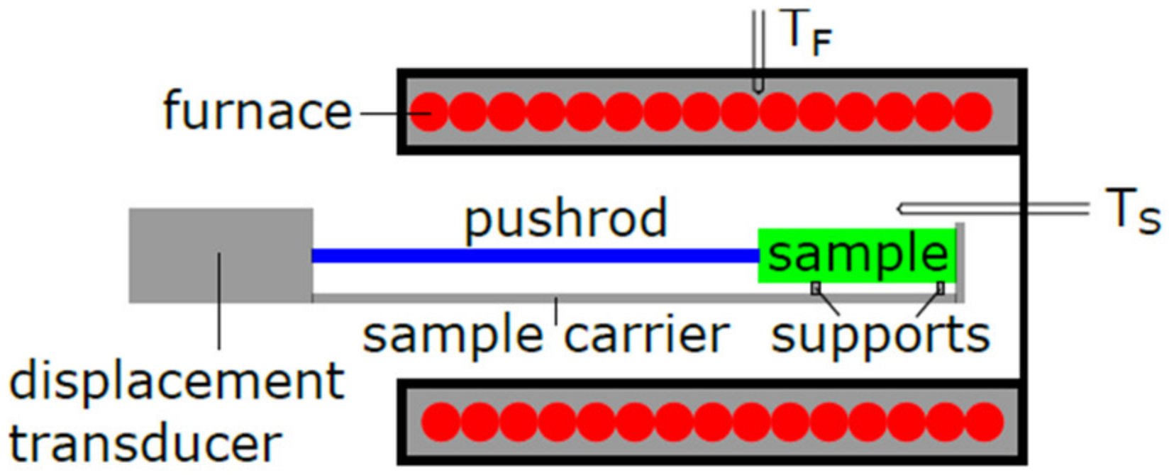
Push rod dilatometry is a specific method of dilatometry to determine the linear thermal expansion of a solid as a function of temperature.
In this work a NETZSCH DIL 402 C (NETZSCH-Gerätebau GmbH, Selb, Germany) (
Figure 7) with a SiC furnace (
Tmax = 1600 °C) with an alumina sample holder, push rod, and sample carrier was used. This system had a measuring range of 5 mm and the linear variable displacement transformer (LVDT) was based on electromagnetic induction and had a resolution of 1.25 nm per digit.
When the sample was heated, the thermal expansion of the sample led to the displacement of the push rod, which was recorded by the displacement transducer. Furthermore, the temperature at the sample was recorded during the whole measurement run. It must be noticed that all built-in components (sample carrier, push rod, supports) expanded during the heating period in the furnace. As such, a correction function was necessary to separate both expansion behaviors. Additionally, the push rod had to “push” the sample with a minimal force to ensure contact between the sample and the push rod.
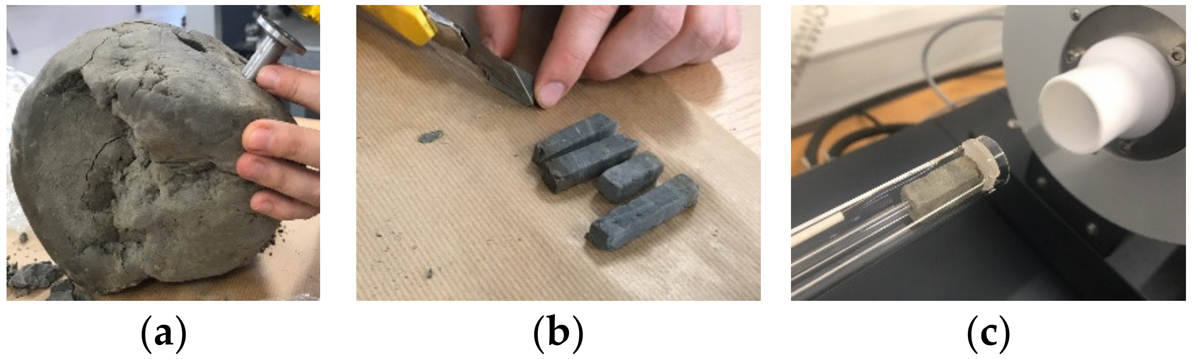
2.4.2. Sample Preparation
The samples for thermal expansion measurements were prepared from 4 different drill core depths. For each depth, at least three samples in the axial, and three samples in radial directions, were prepared and measured in their moist states (s.
Figure 8).
In the second measurement run, samples were dried in a lab furnace at T = 105 °C until no more mass changes were detected.
The sample length in the direction of the dilatometer measurement was L0 ≈ 25 mm while the square cross section had a dimension of approx. 8 × 8 mm. The sample density of the moist and dry states corresponded to the measured densities of the HFM samples, as already mentioned.
2.4.3. Measurement Procedure
The linear thermal expansion measurement for the moist samples was conducted in a temperature ranges from Tmin = −10 °C to Tmax = 80 °C in two subsequent heating and cooling cycles. The heating and cooling rates were defined with β = 2.5 K min−1 to avoid thermal gradients in the sample and an additional flow rate of He gas was applied during the whole measurement run to ensure the removal of the moisture from the sample chamber.
The dried samples were measured with the same temperature program, except for the second heating and cooling cycles.
Before linear thermal expansion measurement of the samples, a correction measurement based on a sapphire standard reference material with L0 = 24,983 mm was conducted.
2.4.4. Evaluation
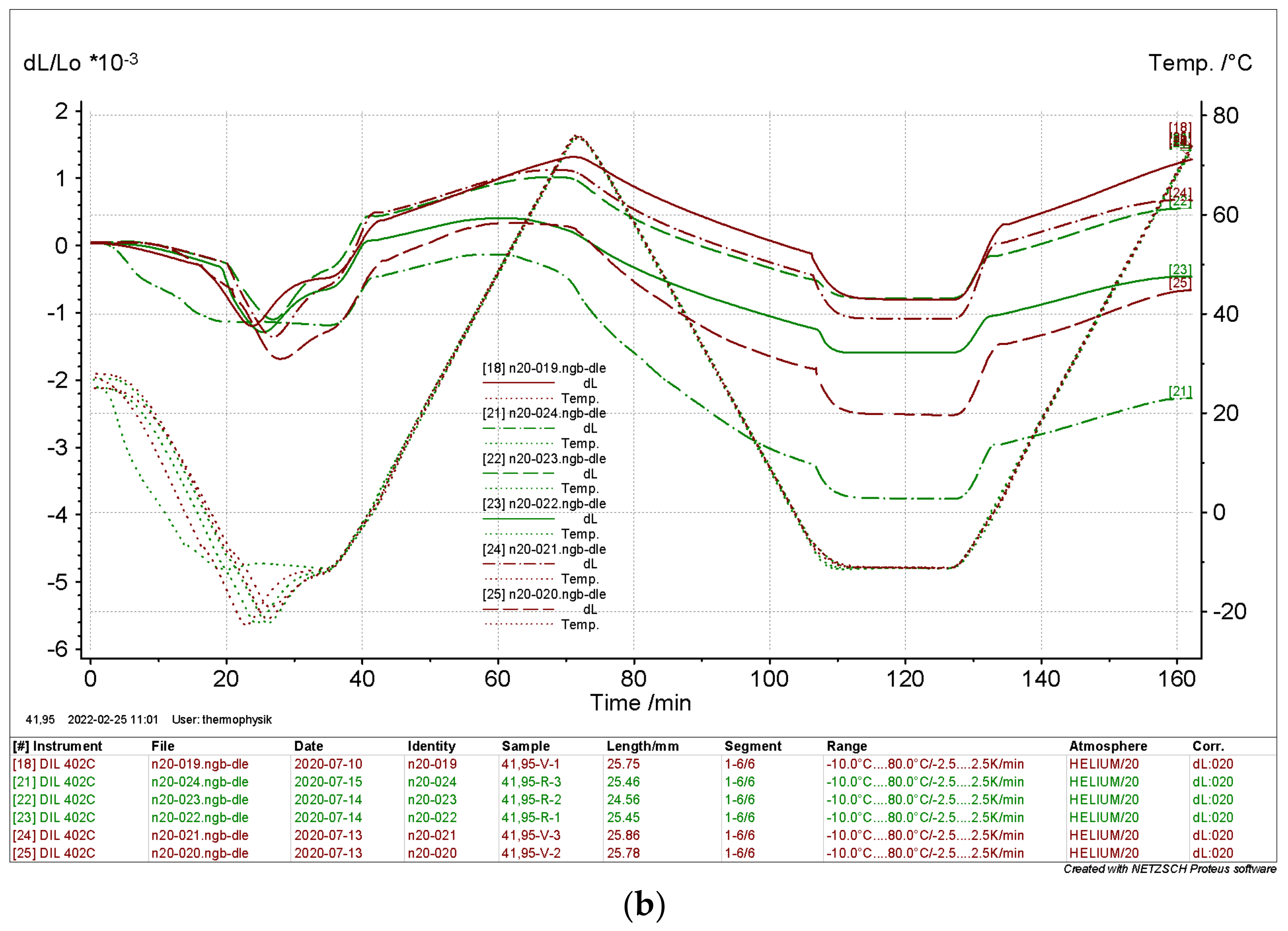
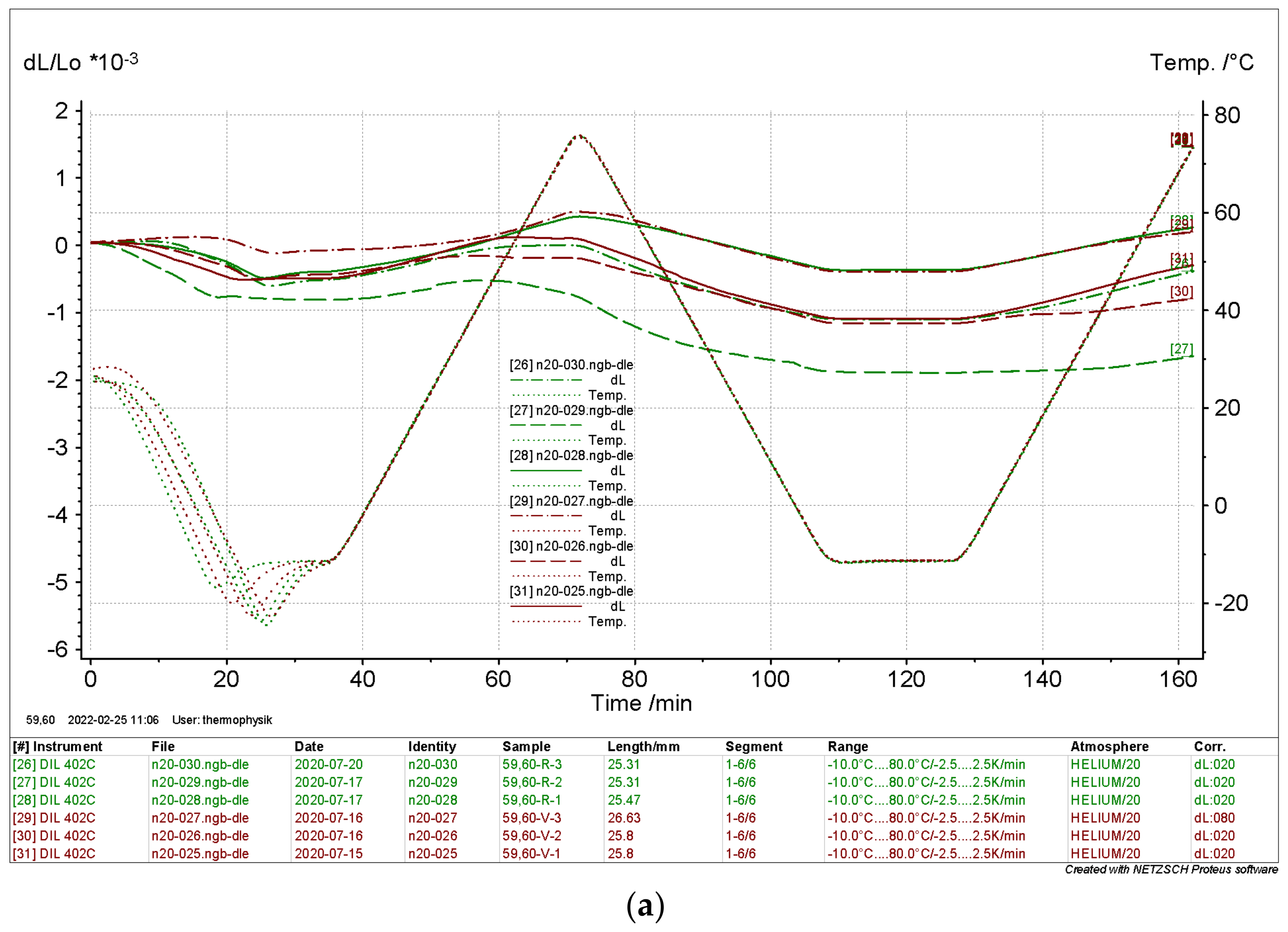
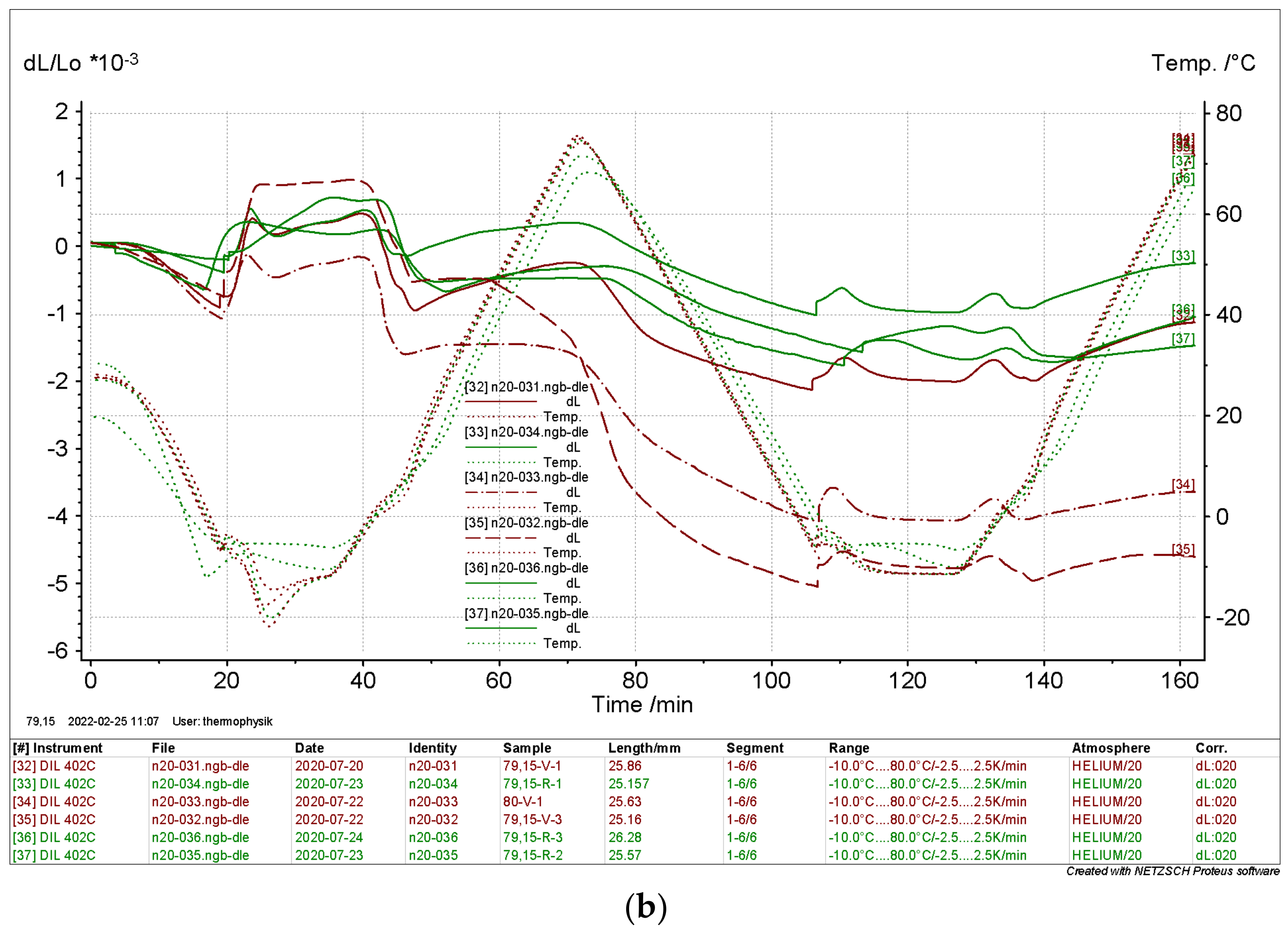
The measured data are represented for each individual sample, where the thermal expansion curves are shown as the relative length change to the initial length in [ΔL L0−1] = 1 and the temperature at the thermocouple is close to the sample in [T] = °C versus time [t] = min.
3. Results and Discussion
3.1. Heat Flow Meter Samples
In sum, eight samples were prepared from the drill core for HFM measurements.
Table 2 summarizes the samples and their dimensional and mass properties.
After the preparation and measurement of the effective thermal conductivity of the moist samples, subsequent drying in the lab furnace was conducted. Thereafter, the dimensions and masses were measured again, and the density of the dry samples was determined, as shown in
Table 3.
In
Table 4, the averaged densities of the moist and dried samples, as well as the relative mass change after the drying process, are shown.
Drying of the drill core segment HFM samples shows the different moisture contents of the segments, depending on the depth. While the samples at 59.42–59.60 m only lost 5.39% of their moisture, the samples at 20.33–20.5 m depth showed a water content of 25.11%.
3.2. Effective Thermal Conductivity and Specific Heat Capacity
Following figures represent the results of the determined effective thermal conductivity, , based on HFM experiments, and specific heat capacity based on the DSC experiments.
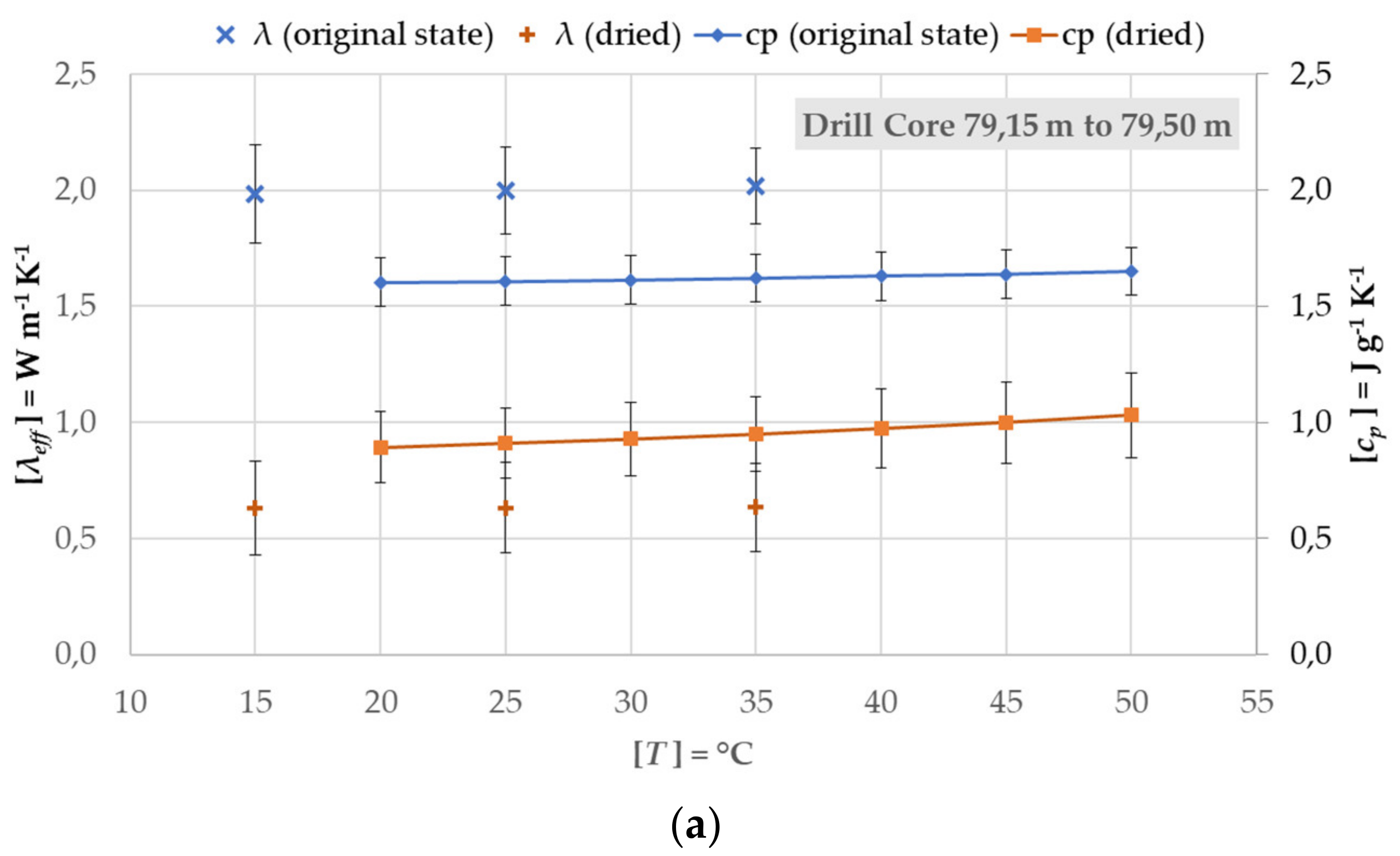
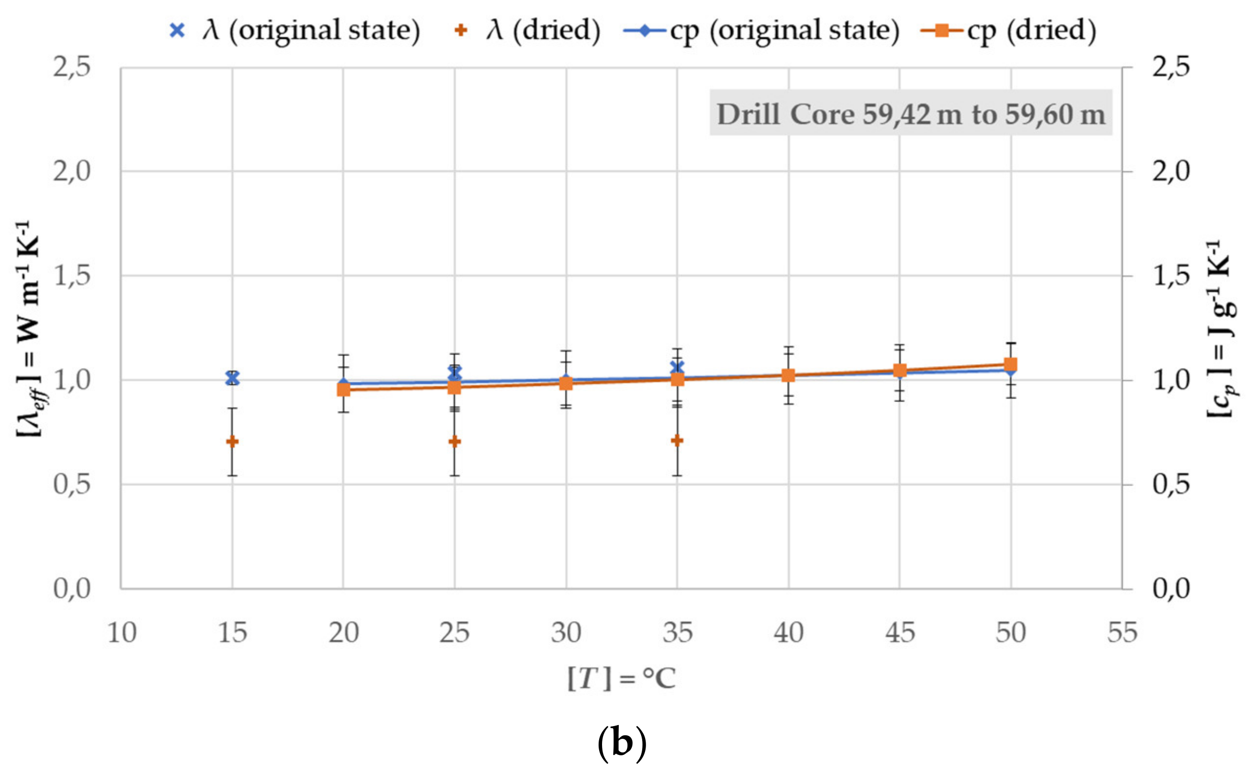
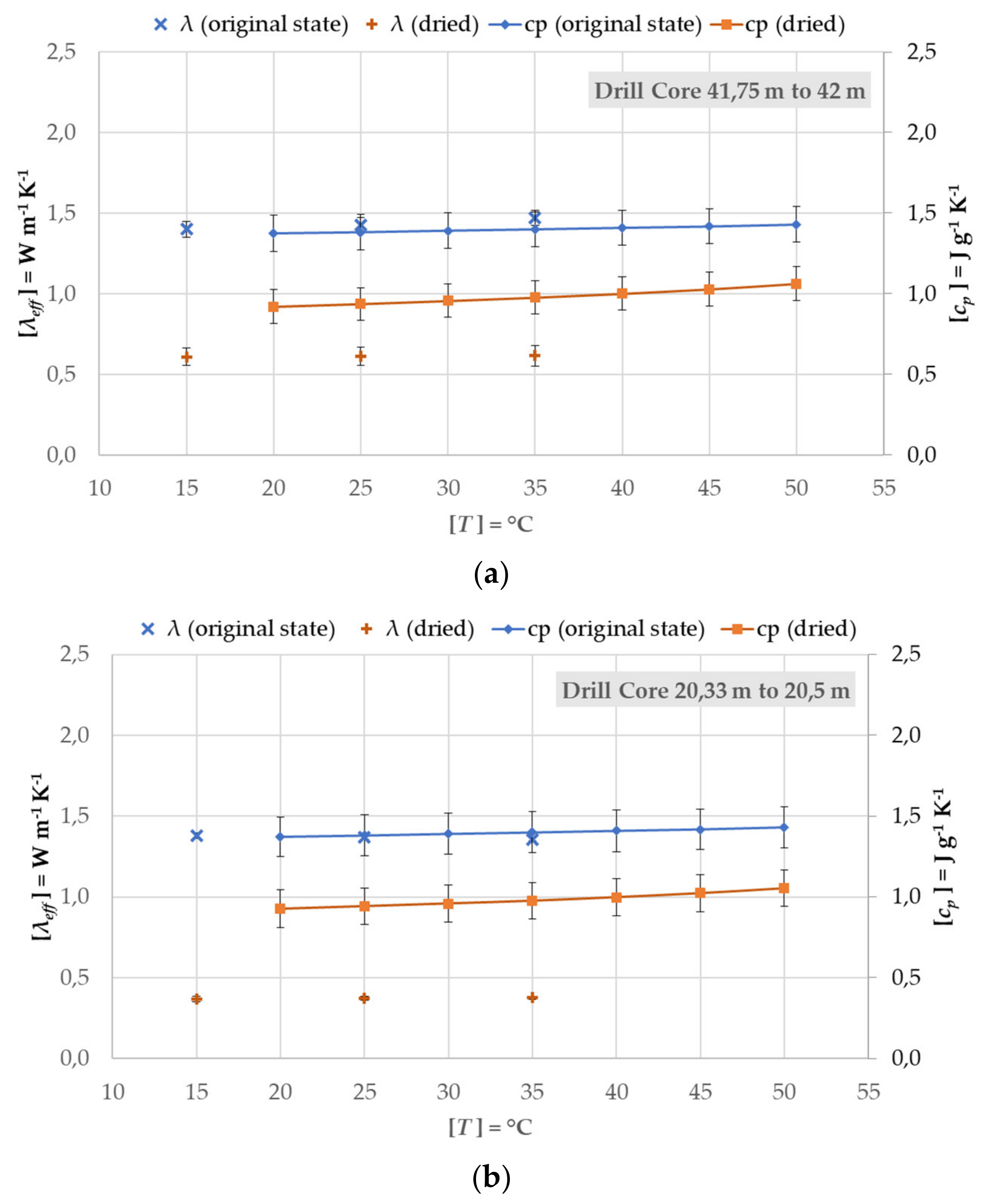
Figure 9 and
Figure 10 represent the determined effective thermal conductivity and specific heat capacity results for the drill core segments in the moist and dry states at four different depths. The actual moisture of the sample had a great influence on both physical quantities. This difference is clearly visible in the measurements of the segments at 79.15–79.5 m and 59.42–59.6 m. The uncertainty bars show the combined expanded uncertainty of all sample measurements, including the device, calibration, and sample uncertainties. The largest influence of these uncertainties come from the samples themselves and are, therefore, very small in the measurement of the effective thermal conductivity at 22.33–20.5 m, since only one sample was available.
A comparison of the data at 79.15 to 79.5 m depths shows that the effective thermal conductivity of the moist sample was but only for the dry sample. The for the dry samples at all depths varied between and while for the moist samples these values varied between and 2.02 .
Specific heat capacity measurements of the dry samples at all depths showed a value of to from to . For the moist samples, these values varied between .
3.3. Thermal Expansion
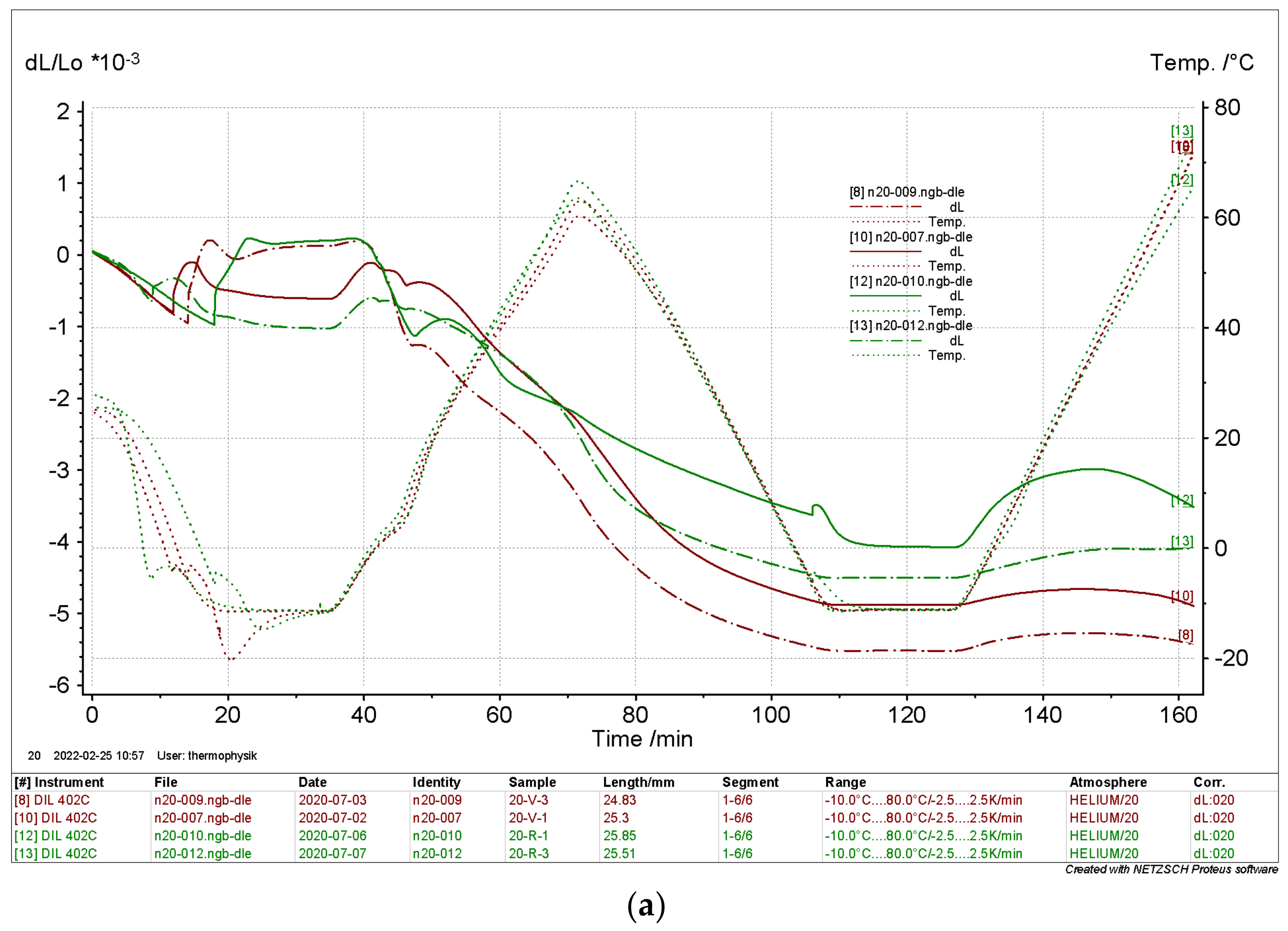
In the following figures represent the results of the thermal expansion measurements of the moist drill core samples from four different depths.
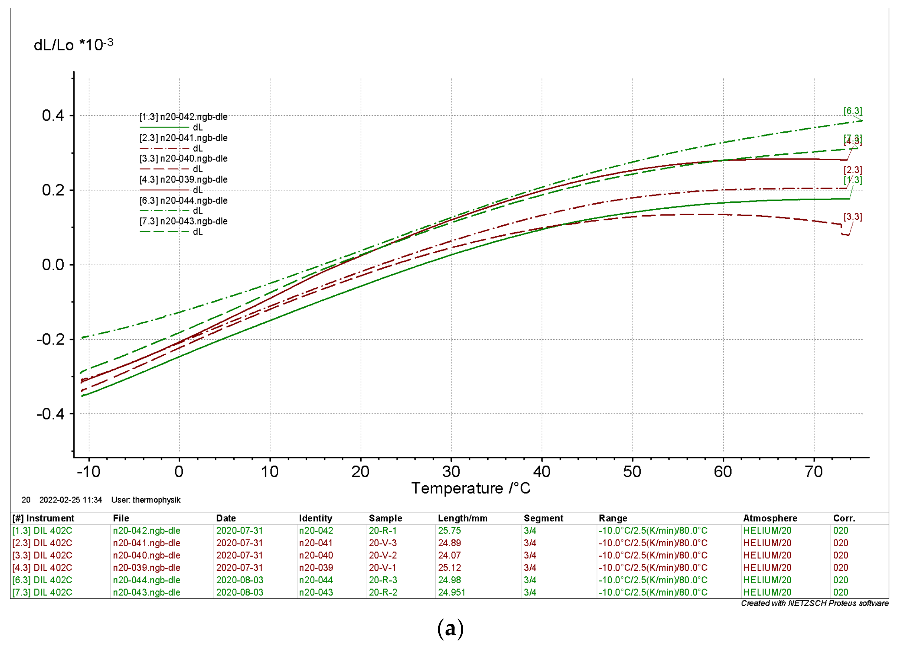
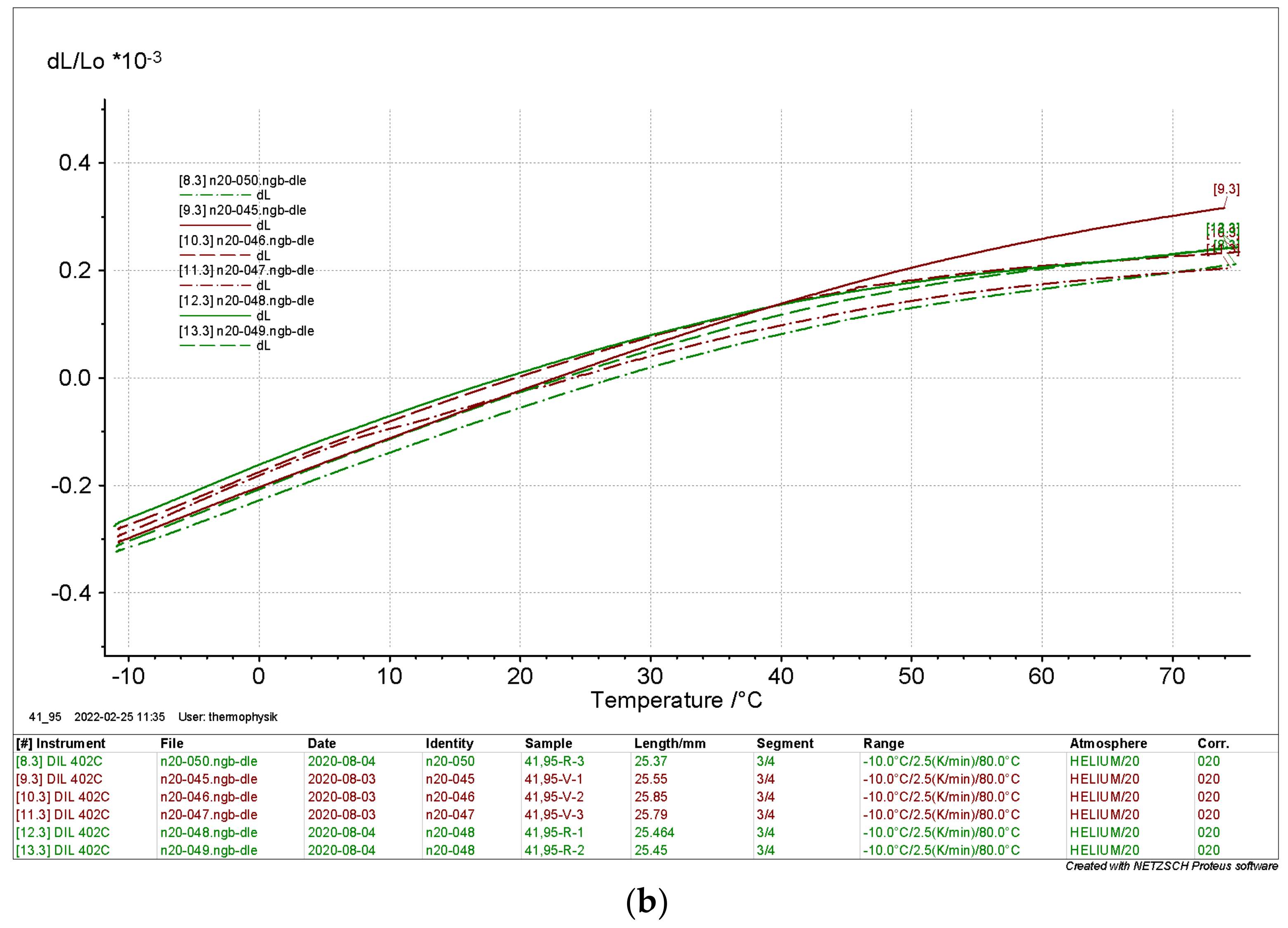
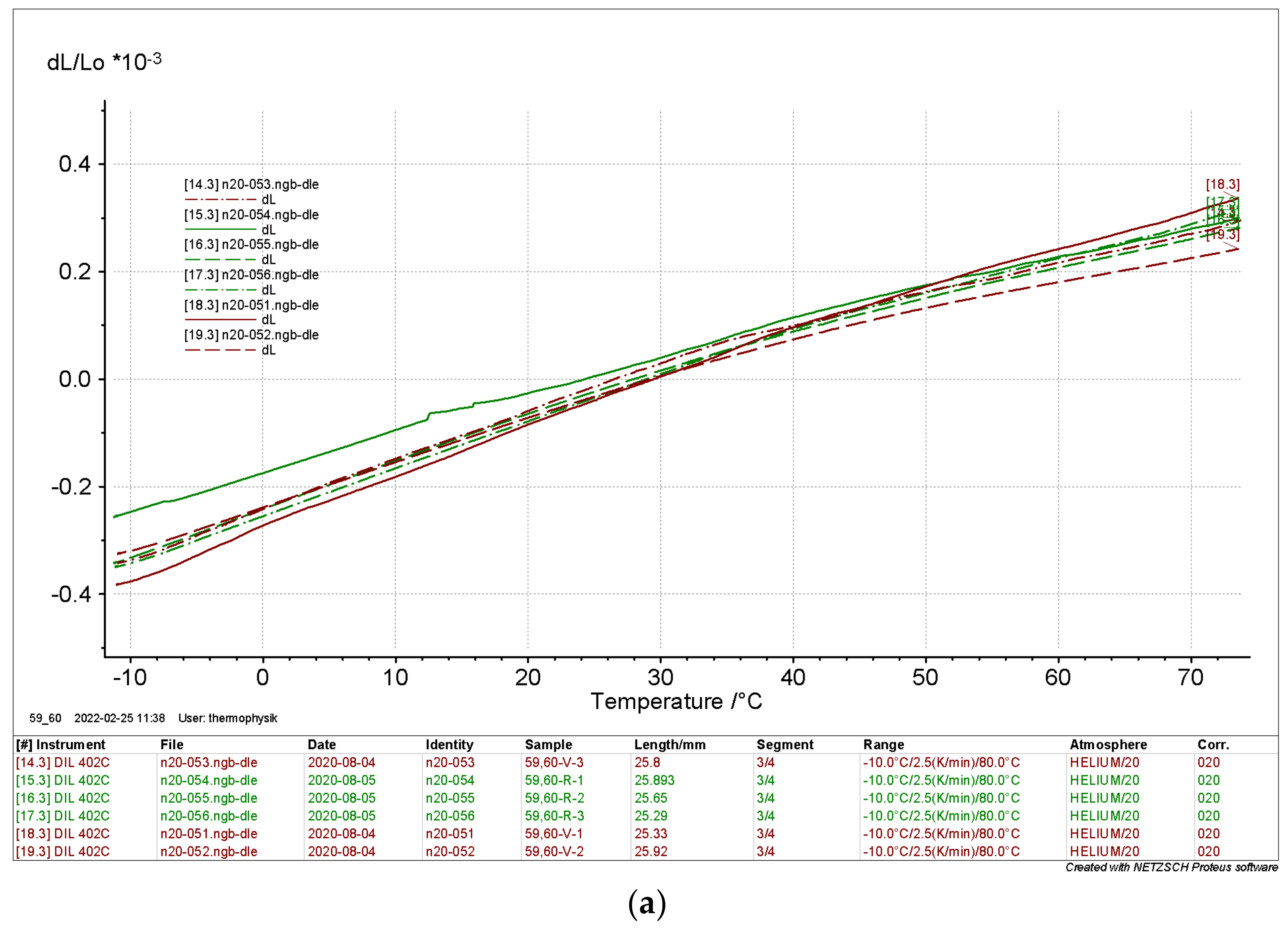
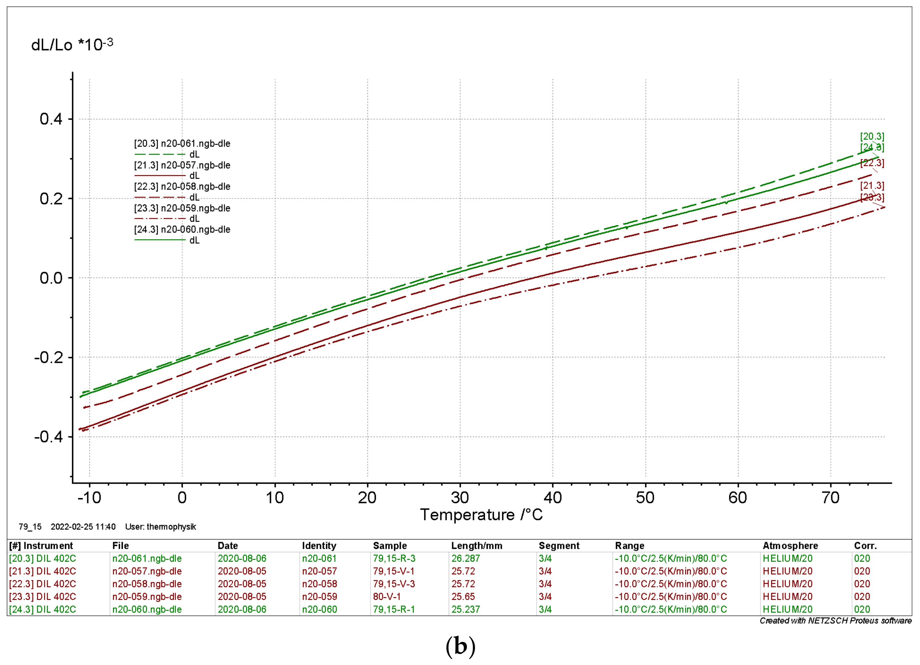
Figure 11 and
Figure 12 depict the relative thermal expansion behaviors of the drill core samples from different depths. The relative length change for the axial (red) and radial (green) samples show no significant difference at all four different depths. The samples at 20 m and 79.15 m mainly showed shrinkage of the overall sample length, while the samples at 41.95 m and 59.6 m showed expansions at the heating segment and shrinkage in the cooling segments in the measurement procedures. The first cooling and heating cycle showed, for the 20 m depth and 79.15 m depth at approx. 0 °C, spontaneous changes of the relative length changes that might be a volume change due to the phase change of the water. The same curves consistently showed greater shrinkage in subsequent heating and cooling segments, which may be attributed to drying shrinkage. In the 2nd heating cycle, all specimens showed expansion behavior, except for the specimens from the 79.15 m depth.
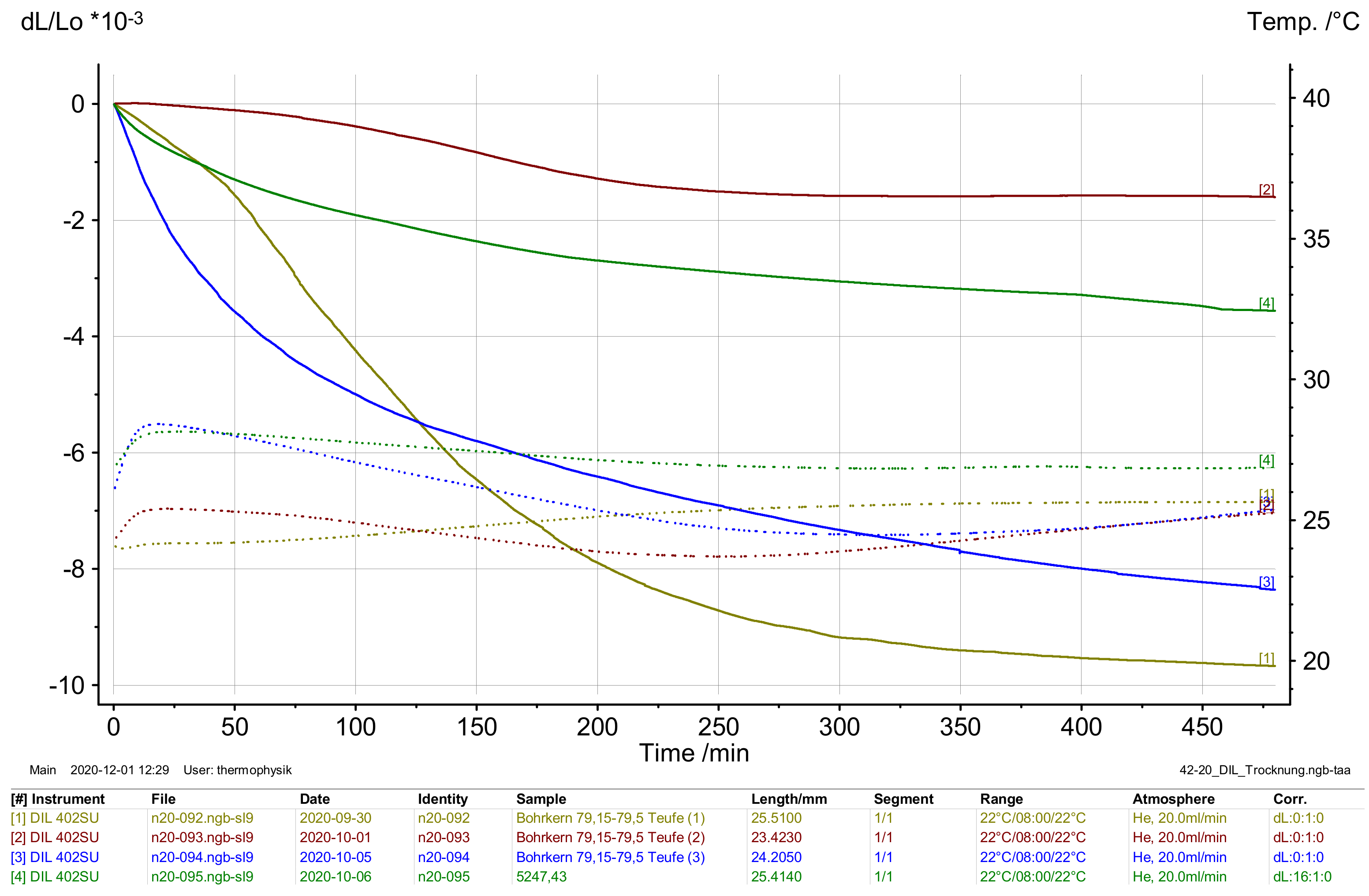
Due to the strong deviation in the results, four additional samples from the 79.15 m depth were measured using the same conditions as the previous dilatometer measurements. The difference in these additional measurements was that no temperature program was applied and only the relative length change at room temperature was recorded. The intention of this additional experiment was to focus on the drying of the sample and the impact on the relative length change without an additional heat source.
Table 5 reports the sample masses before and after the experiment.
Figure 13 represents the results of the relative length change. Both results, the relative thermal expansion and the mass change at room temperature, strongly support the view that inhomogeneous moisture content and different drying kinetics lead to incomparable length change data for the moist samples. The drying shrinkage superimposed the thermal expansion of the material.
Due to this, additional experiments on dry drill core segments were conducted, as shown in the following figures.
The results depicted in
Figure 14 and
Figure 15 clearly show that the relative length change of the dry samples differed significantly from the results of the moist samples. Again, there is no significant evidence of the directionality of the samples. The curves indicate a thermal expansion in the range of Δ
L L0−1 ≈ 0.8 × 10
−3 in a range from
Tmin = −10 °C to
Tmax = 80 °C. The moist samples differed considerably with Δ
L L0−1 ≈ 2 × 10
−3 to 6 × 10
−3.
4. Conclusions
The work demonstrated that the HFM method can be used to determine the effective thermal conductivity of drill core segments. Uncertainties of measuring device, as well as associated calibrations, are much smaller than the scatter of effective thermal conductivity data from several samples. Drying can be prevented through hermitically sealing to determine the effective thermal conductivity in the moist state of samples.
The determination of the specific heat capacity of the drilled core samples, by means of standardized DSC measurements, showed that the samples themselves are the main share of the total measurement uncertainty budget and that instrument and calibration uncertainties, on the other hand, are small.
In addition, the temperature dependence of the specific heat capacity and the effective thermal conductivity could be determined with both applied methods. In the selected temperature range of 15–50 °C, the measured mean values of the effective thermal conductivity and specific heat capacity show only a slight increase in temperature in terms of the uncertainty range of the measurement itself.
The results from the thermal expansion measurements showed the strong influence of sample moisture and drying of the measured drill core segments on the actual expansion behavior in a temperature range from −20 to 80 °C. The change in the length of the specimens, due to drying shrinkage itself, overlapped the expansion measurements since no hermetic sealing of specimens was possible in this case. The actual thermal expansion strain could only be measured from dried specimens, and was ΔL L0−1 ≈ 0.8 × 10⁻³ for all investigated depths.
Our findings support the view that the actual moisture content of a subsoil sample has a strong impact on the thermal conductivity, as well as heat capacity and thermal expansion. From these results, the main soil thermal properties for the investigated drill cores could be determined and, thus, demonstrates the applicability, especially of the HFM method, on drill core sections.
Future research should use the evaluated thermal properties of soil to calculate the temperature field of a BHE and its surroundings in spatially resolved and transient simulations. Finally, a more sophisticated method of sample preparation, as well as measurement procedures, must be developed to maintain the moisture content of samples for thermal expansion measurements.


