1. Introduction
The conditions of chemical equilibrium shifts in the systems with single chemical reaction were elaborated in the classical thermodynamic works and are well-known as Le Chatelier-Braun principle or simply Le Chatelier principle. This principle was repeatedly supplemented, justified, and commented on in a number of thermodynamic works, for example, classical monographs [
1,
2,
3,
4,
5,
6,
7]. Aside from the original author of the principle (Le Chatelier’s original article is [
8]), it should be noted the fundamental role of J. W. Gibbs in substantiating this principle [
4,
5,
6]. The authors consider the presentation in the monograph [
9] to be the most successful in terms of simplicity, consistency, and generality.
The following paragraph was inserted into Introduction. Let us allow ourselves a digression related to the prehistory of the issue. The principle of Le Chatelier—Brown itself was formulated in 1884 “If a system in stable equilibrium is acted upon from the outside, changing any of the equilibrium conditions (temperature, pressure, concentration, external electromagnetic field etc), then the processes directed to side of resistance to change”. Henri Le Chatelier (France) formulated this thermodynamic principle of moving equilibrium, later generalized by Karl Braun. The principle is applicable to equilibrium of any nature: mechanical, thermal, chemical, and electrical. If external conditions change, this leads to a change in the equilibrium concentrations of substances. In this case, one speaks of a violation or shift in chemical equilibrium. The chemical equilibrium shifts in one direction or another when any of the following parameters change:
temperature of the system, that is, when it is heated or cooled;
pressure in the system, that is, when it is compressed or expanded;
concentration of one of the participants in the reversible reaction.
All these variants of external influences are considered in this article. This principle, in an exceptionally simple and illustrative form, formulates the direction of displacement of the equilibrium state under external action on the system and is truly universal. Despite the fact that the principle itself was formulated a very long time ago and is very well known, the authors dare to assume that they propose some (albeit not too significant) change and expansion of the interpretation of the original principle stated earlier by the authors-Henri Le Chatelier and Karl Braun.
In the opinion of the authors, the scientific novelty of the presented work consists of two main aspects:
- (A)
Attempts to extend the well-known principle of shifting chemical equilibrium to systems, in the case of the initial substances or reaction products belonging to phases with large (sometimes extremely large) positive deviations from ideality. In these cases, the contribution of the excess partial thermodynamic functions of the components to the equilibrium shift may be comparable and even exceed the contribution of the standard thermodynamic functions of the reaction participants. This aspect, in the opinion of the authors, has not been considered before.
- (B)
Attempts to extend the well-known principle of shifting chemical equilibrium to systems of several chemical reactions with common reagents, products, or intermediates. In these cases, there is competition between several chemical reactions for both participants in the reaction, and the displacement of the equilibrium in one reaction affects the displacement of the equilibrium in the other reaction. This aspect has not been considered before, as far as the authors know.
Thus, the main goal and results of this work was an attempt to extend the well-known principle of equilibrium displacement to complex interrelated chemical processes occurring in highly nonideal systems. The methodology of consideration, in the opinion of the authors, is quite traditional and corresponds to the general principles of chemical thermodynamics. The poet does not need an additional description.
We also included links to the latest works for 2021 and 2022 in the text (see, for example articles [
10,
11]). These works (as well as earlier ones) were carried out within the framework of the standard and generally accepted methodology in thermodynamics.
2. Isolated “Free” Reaction Systems
Let us consider isolated equilibrium reactions, where reactions have no common reagents or products. This allows us to consider any reaction separately without taking into account other reactions.
Let us consider equilibrium chemical reaction:
where
is stoichiometric coefficient of molecular
in reaction (1),
and
are number of reagents and number of all participants in the reaction (1). Assume, that
We can simplify Equation (1):
Differential equation of chemical equilibrium conservation will be the following:
Differentiating Equation (4) by temperature
(T), pressure
(P), and molar number of all components
, we get the expression:
where
In Equations (6)–(10):
are partial molar entropy, partial molar volume and enthalpy of
i-th component;
is chemical affinity of reaction (3),
is its chemical variable, and
. According to the physical sense,
are change of entropy, volume, chemical affinity, and Gibbs energy in the isotherm-isobaric process of the formation of
moles of product
from
moles of reagent
in the mixed phase (or phases) with infinitely large mass, which contains both reagents and products. According to the sense of
According to Sylvester’s criterion, because determinant of the matrix of second derivatives is positive,
where upper index symbolizes determinant dimension. All minors of main diagonal of
are positive also.
According to the criterion of phase diffusional stability with respect to infinitesimal state changes. Thus, one can directly determine the signs of the derivatives:
3. Once Connected “Un-Free” Reaction Systems
Before consideration of the connection by common reagents or products, equilibrium chemical reaction let us formulate an obvious lemma.
Lemma. If any chemical reactions are carried out in the chemically equilibrium reaction phase (we will call them natural reactions or simply reactions), then any linear combinations of these reactions are carried out there (we will call them quasi-reactions).
Let
k be the number of reactions. If for
j-th reaction,
;
has arbitrary sign or may be equal to zero.
Here is the simplest example of 2 connected reactions:
We treat the reaction phase as a “black box” in which we placed a single reagent, A, and then discovered two more products, B and C. If we do not consider the mechanism of the reactions, then we are deprived of the opportunity to figure out how the sum process proceeded:
as a combination of two 1 and 2 reactions;
as 1 quasi-reaction;
as a combination of any reaction with 1 quasi-reaction;
as a combination of any reaction with 2 or 3 quasi-reaction.
The last variant may be realized according to schemes:
Naturally, all changes of state functions in such quasi-reactions (
) should be linear combinations of changes of state functions in these reactions (
) with the same coefficients:
4. Un-Free Connected Reactions
Let us consider once connected “un-free” equilibrium reactions, where two or more reactions have common reagents or products, or reagent of one reaction is the product of the other. Consider a pair of connected reactions. This will allow us to consider the competition between two connected reactions for the supplied thermal energy and mechanical energy (relative shift of chemical equilibrium when temperature or pressure changes).
4.1. Case of Common Reagents or Common Products
where is stoichiometric coefficient of molecular in reaction (j), n are number of all participants in both reactions (1 and 2). Assume, that:
for products;
for reagents;
for compounds, not involved in the j-th reaction.
Assign a number 1 to the common participant of 1 and 2 reaction and divide reaction-1 to
and reaction-2 to
. Therefore, Equations (32) and (33) may be rewritten as:
where:
Then, we subtract from the Equations (34) and (35):
where:
According to previous terminology, a quasi-reaction (37) is isolated and can be considered the way as in
Section 1.
Again note that:
according to Sylvester’s criterion, because the determinant of the matrix of second derivatives and all minors of main diagonals are positive.
Thus, to formulate the corollaries of Equation (44):
To verbally formulate the Le Chatelier’s principle of chemical equilibrium shift (CES-principle):
With an increase in temperature for a pair of once-connected reactions, the equilibrium shifts towards products more (less) for the reaction, whose specific heat (normalized by 1 mole of the common component) is greater (lower) than the other reaction;
With an increase in pressure for a pair of once-connected reactions, the equilibrium shifts towards products more (less) for the reaction, whose specific volume change (normalized by 1 mole of the common component) is lower (greater) than the other reaction;
If there is a system of
q once connected equilibrium reactions (it is not necessary that the common products or reagents are the same), we can consider a system of independent pairwise quasi reactions of the type (37) without common participants. One can write the following equation system:
where
. All corollaries of the type (47)–(49) will also be valid. All
q reactions should be linearly independent, so the rang of matrix of stoichiometric coefficients for the reaction system
with the dimension
nq should be:
All quasi-reactions naturally are linearly dependent on the reaction system.
4.2. Case of Common Reagent of One Reaction and Product of Other Reaction
Let us consider the system of sequential reactions. Assign again a number 1 to the common participant of the reactions (product for reaction-1, and reagent for reaction-2) and divide reaction-1 to
and reaction-2 to
. Therefore, Equations (34) and (35) maybe be rewritten, as earlier:
where again:
We then add Equations (52) and (53) and exclude 1 component from quasi-reaction:
and contrast with Equation (38):
According to previous terminology, quasi-reactions are isolated and can be considered as previously in
Section 3. Thus:
where:
Naturally, the positive definiteness of the bilinear form (45) is also valid in this case:
Note also, that if:
then:
In other words, equilibrium molar numbers of common components in the reactions-1,2 increases, decreases, and becomes constant. We then formulated the corollaries of Equation (57), which completely matched with the Equations (47)–(49), excluding the signs in definitions in the Equations (39)–(43) and (58)–(62).
With an increase in temperature for a pair of once-connected reactions, common component-intermediate was accumulated (consumed) in the reaction phase, if sum heat of the reactions (normalized by 1 mole of the common component) was positive (negative);
With an increase in pressure for a pair of once-connected reactions, the common component-intermediate was accumulated (consumed) in the reaction phase, if sum volume change of the reactions (normalized by 1 mole of the common component) was negative (positive).
Let us give examples of the reactions (for example in A3-B5 systems), once-connected by:
reagents:
products:
sequential reaction:
5. Case of Several (More Than One) Common Reagents or Common Products with the Proportional (in Particular, Equal) Stoichiometric Coefficients of Common Participants
Let us give examples of multi-connected (by products or reagents) reactions with equal stoichiometric coefficients for participants. Let us give the example:
In a common case, we will denote all common participants for two reactions as 1, 2…k. We can hardly imagine a pair of connected reactions where the number of connected components would be
k > 3, so reactions are twice or thrice connected.
In this case, similarly to what we did in
Section 3, we can exclude common participants from the reactions, form quasi-reactions, and get all the conclusions, which completely match with the Equations (47)–(49) (CES-principle). A quasi-reaction is naturally formed as a sum (not difference) of equilibrium reactions, and the result is a result similar to the one previously obtained in
Section 3.
6. About the Possibility of Passing of Composition Variables, Temperature, and Pressure in the System of Components, Connected by Chemical Reaction, through the Extreme
Isotherm-isobar conditions
Let us assign the number 1 to the common component. Imagine that molar number of some non-common 2-d participant of the
1-st from pair of (1 and 2) once-connected reactions
(n2(1)) passes through the extreme at P=const and T=const. Naturally in these cases:
Let us use it now in Equation (57) for such reactions at
P = const and T = const:In other words, molar numbers of all participants of the reactions-1,2 pass through the extreme at
P = const and
T = const simultaneously. If quasi-reaction-1,2 (pair of once-connected reactions-1 and -2) is connected with the other
(−1r) or
(−2t) quasi-reactions by one common component (it is not necessary that the same as for quasi-reaction)-1,2, then the following is also valid:
Thus, one can postulate that the condition of the extreme of molar numbers of the participants of chemical reactions or the condition of extreme of chemical variable in the system of once-connected equilibrium chemical reactions is transmitted from one reaction to another reaction through a common participant in the reaction. The same conclusion was made for twice or thrice connected to each other reactions, with proportional stoichiometric coefficients of common participants. Unfortunately, in more complex cases of connected reactions, the authors fail to establish the transmission of the extremeness of the composition.
Transfer of the condition of extremeness of the composition from one connected reaction to another can be explained, if we take into account that when the composition changes, there is competition between connected reactions for a common reagent or common product.
One important moment. In our system of connected reactions should be the components not involved in the connected reactions at T, P = const. Otherwise, the number of thermodynamic degrees of freedom will be equal to zero, and system will be non-variant.
We will give the simplest scheme of extreme transfer between connected reactions as an example. Let us consider the reactions scheme at P = const and T = const:
According to chemical equilibrium shift differential equation, one can write that when
:
In our conditions, when
then:
or all molar numbers simultaneously pass through the extreme.
At the same time, there should be some other components in the systems,
F, G, H…, for which:
Condition of constancy of chemical potentials of components, which also corresponds to the Equation (75), may also be valid. However, for some components, according to the conditions of diffusional stability, derivatives should be:
Therefore, input (or output) of not those involved in the connected reactions components to the reaction phase cannot make chemical potentials of the last ones constant.
Reaction phase composition may change in different ways: adding or removing component or components (products or reagents) in real experiment, for example, moving along isotherm-isobar curves of multi-phase equilibrium (also in experiment or in correct thermodynamic modeling calculation); moving along curves of open phase processes (when one from several equilibrium phase it is constantly being removed from the sphere of phase equilibrium); and moving along curves of thermodynamic simplification or curves of incomplete extremes etc. (see, for example [
9]). In the last cases, it is enough to change in the experiment, the gross composition of heterogeneous system as a whole.
For simplicity and certainty, in the condition of isotherm-isobar composition changes, we shall fix the total number of moles of all components in the reaction phase equal to 1 mole. Then, components molar numbers will convert into molar fractions, , with the conservation all equations and properties of the reaction phase. All extensive properties in the system will transfer into molar properties, in particular, determinant , losing dimension by one, remains defined positively with all minors of main diagonal, etc.
In the end of the section, we will give an example of the experiment, where concentrations of participants of the connected reaction simultaneously pass through the extreme (
Figure 1). Here, the composition change is caused by artificial displacement of melt composition along liquidus isotherm in quaternary
In-Ga-As-Sb system and corresponding change of equilibrium solid solution
InxGa1/2-xAsySb1/2-y composition.
6.1. Polytherm Isobar Conditions
Driving force of chemical equilibrium shift is heat supply or removal in the conditions of mass isolation of the reaction phase. If we consider isolated reactions, then Equation (5) will be:
and we can postulate, that:
Really:
because the thermal diffusional criterion of the reaction phase is valid, i.e.,:
, when heat is supplied or removed.
Connected reaction systems. Let us number common components in the
1-st. Imagine that molar number of some non-common
2-d participant of the 1-st from pair of (1 and 2) once-connected reactions passes through the extreme at
P = const. Naturally, in these cases:
For the 1-st reaction we can also rewrite Equation (5):
From Equations (83) and (84), we can write that:
Using Equations (43) and (44) for quasi-reaction-12 at
P = const:Taking into account Equation (85), one can write that:
is in the extreme, and from Equations (83) and (86) it follows that:
We can postulate that molar number of all participants of the (12) connected reactions and temperature of the reactions pass through the extreme at
P = const simultaneously.
At the end of the section, we will give an example of an experiment where concentrations of participants of the connected reaction and temperature simultaneously passed through the extreme (
Figure 2). Here, the composition change was caused by artificial displacement of melt composition along liquidus polytherm in quaternary system
In-Ga-As-Sb. In this case, the composition of solid solution was fixed in
In0.11Ga0.39As0.08Sb0.42. This composition corresponds to the pass of the concentrations in solid solution through the extreme, and this applies both to the simple components
A3(
In, Ga) and
B5(
As, Sb), and “complex compounds”
A3B5 (InAs, InSb, GaAs, GaSb), as seen in
Figure 1. These data also correspond to the value of the argument,
. Temperature of phase equilibrium in
Figure 1 (873 K) should correspond to the extreme of liquidus temperature at the same value
. This is confirmed by
Figure 2. Justice of Equation (88) was demonstrated.
6.2. Isotherm Polybar Conditions
The driving force of chemical equilibrium shift is reaction volume increase or decrease in the conditions of mass isolation of the reaction phase. Imagine that molar number of some non-common
2-d participant of the 1-st from pair of (1 and 2) once-connected reactions passes through the extreme at
T = const. Naturally, in these cases:
If we consider isolated reactions, then Equation (5) will be the following:
From Equations (89) and (90), we can write that:
Really:
because the mechanical diffusional criterion of the reaction phase is valid, i.e.,:
.
In reality, condition (91) is incomparably milder than a similar condition (81). For example, the condition is certainly fulfilled for the reaction in ideal gaseous phase (when molar gaseous numbers of reagents and products are equal). This condition is also approximately valid for the reaction in the condensed phases, when pressures are not unnecessarily large.
Connected reaction systems. Using Equations (43) and (44) for quasi-reaction-12 at
T = const:Taking into account Equation (85), one can write that:
is in the extreme, and from Equations (89) and (90), it follows that:
We can postulate that molar number of all participants of the connected 1,2-reactions and pressure of the reaction pass through the extreme at
T = const simultaneously.
The last example of the transmission of the state parameters extreme conditions is represented in
Figure 3 and
Figure 4.
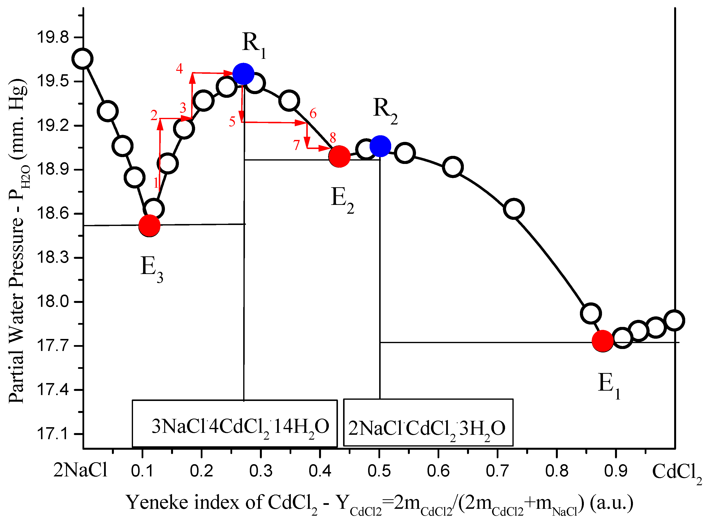
1→2→3→4→R1→5→6→7→8 shows the method of passing the composition of the solution through R1 point as the result of H2O-add +(1→2→3→4→R1) and H2O-evaporation + -crystallization (R1→5→6→7→8).
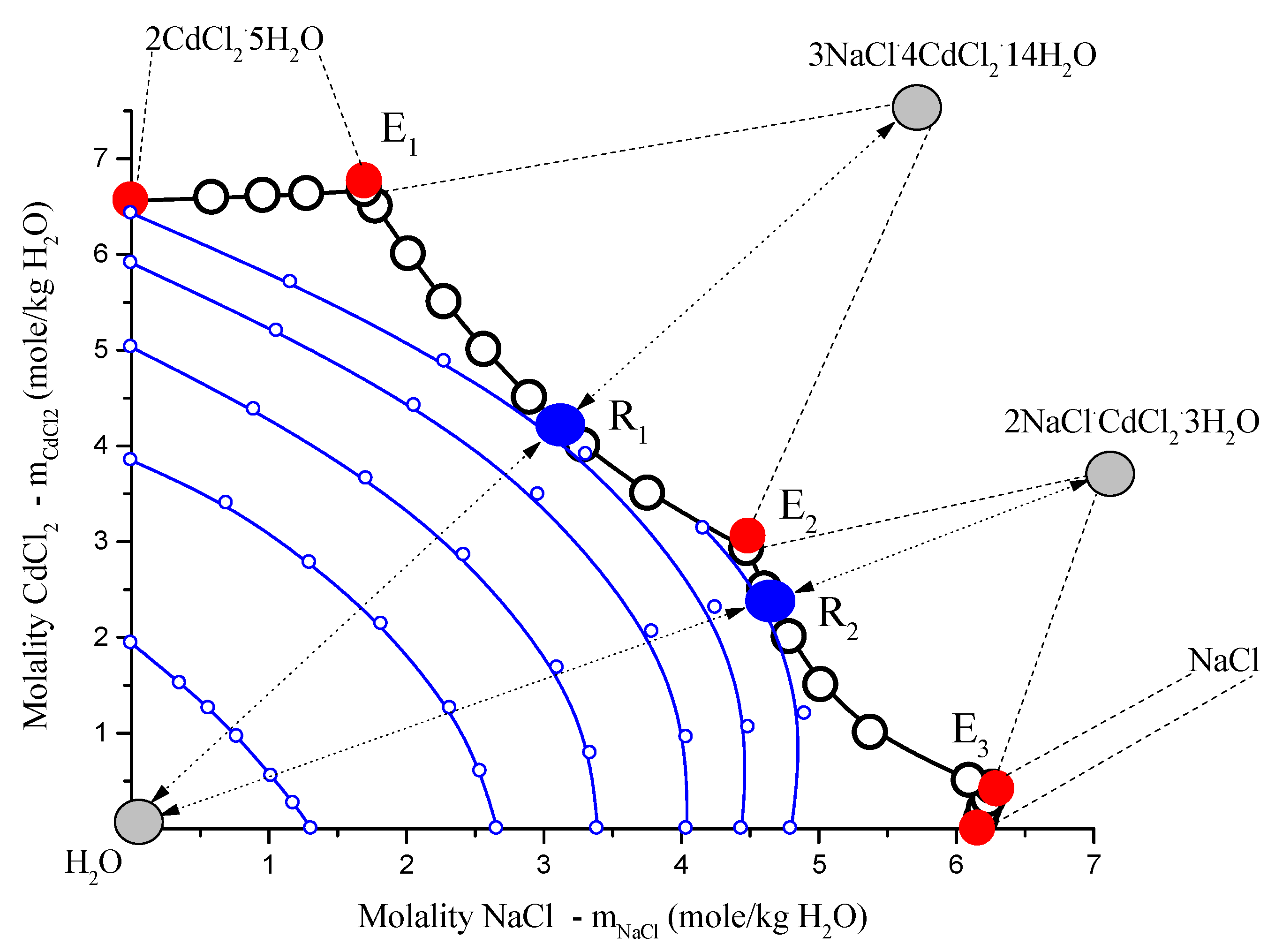
In
Figure 3, isotherm-isobar (1 atm. of sum pressure) of ternary system
NaCl-CdCl2-H2O system at 25 °C consists of four branches:
NaCl; congruently soluble compounds,
, and
. Diagram contains three non-variant points
Ei, all eutonics [
15]. In the diagram, there are two point types. Van Rijn points in fusibility diagrams,
Ri, are realized when all three equilibrium phase points, liquid
(l) (Ri), solid compound
(s) ( and
), and vapor
(v) H2O, belong to the same straight lines [
15,
16,
17]. In the points,
Ri isopotentials of
H2O touch the curves of mono-variant equilibrium
(Ei→Rj→Ei+1) when moving along these curves, and chemical potential
H2O in the points
Ri passes through the extremes (specifically the maximum) [
17,
18], as in
Figure 3 and
Figure 4.
Figure 3.
Solubility diagrams in ternary
NaCl–CdCl2–H2O system at 25 °C in rectangular Schreinemakers concentration triangle in the salt molalities: open black circles, calculated by Extended Pitzer’s Method [
16]; red solid circles, non-variant experimental data [
16,
17]; blue solid points
(Ri), solubility diagram points type Van Rijn points in fusibility diagrams [
17]; little open blue points,
H2O isopotentials (
); gray points, figurative points of coexisting equilibrium vapor
(H2O) and solid compounds phases
c and
;
Ei, eutonics [
17,
18]; dots with two-directed arrows are nodes: vapor
(v), saturated solutions
(Ri), and solid compounds
(s).
Figure 4.
Solubility diagrams in ternary
NaCl–CdCl2–H2O system at 25 °C in the variables: salt Yeneske index
H2O partial pressure: open black circles, calculation by Extended Pitzer’s Method [
14]; red solid circles, non-variant calculated eutonics data (
Ei); blue solid points
(Ri), solubility diagram points type Van Rijn points in fusibility diagrams [
17,
18]; red arrows show the direction.
To describe the behavior of components and molar number during moving liquid composition along curve (for certainty
(E3→R1→E2), imagine a thought experiment. It is possible to organize such process only with mass transfer. In a mass transfer in heterogeneous system or conduct such isotherm-isobar open phase process [
19]:
To the heterogeneous system (liquid is point 1 in
Figure 4), add some liquid
H2O (liquid pass to point 2);
Dissolve part of the equilibrium solid compound in solution until saturation (liquid pass to point 3);
Repeat this two-stage process until liquid comes to the point
R1 (liquid pass to point 4, to point 5, … to point
R1 (
Figure 4);
Evaporate H2O from liquid R1 (liquid pass to point 5);
Crystallize from supersaturated liquid crystals until liquid become saturated (liquid pass to point 6);
Repeat this two-stage process until liquid comes to the point
E2 (liquid pass to point 7, to point 8, … to point
E2), as in
Figure 4.
It is clear, that in the first half of process where
1→2→3→4→R1, molar number dissolved in liquid
increased, so simultaneously increased molar numbers of
in liquid. In the second half of process,
R1→5→6→7→8, molar number dissolved in liquid
decreased, so simultaneously decreased molar numbers of
in liquid. In
R1, molar numbers of
pass through the extreme.
H2O molar numbers in
R1 also pass through the maximum, according to criterion of diffusional liquid stability (values of
H2O chemical potential, activity, and partial pressure always (at
P, T = const) change). It is clear that the compound
’s molar number in the solid phase in
R1 also passes through the extreme. Thus, we have confirmed that molar numbers of the substances were connected by a heterogeneous chemical reaction:
passes through the extreme simultaneously.
To determine the behavior of pressure during moving liquid composition along curve for certainty
(E3→R1→E2), we can use the well-known Gibbs rule [
9,
20]: Temperature (at
P = const) or pressure (at
T = const) passes through the extreme when the composition of equilibrium coexisting phases were linearly dependent. In our case, the three-phase equilibrium figurative points of
(v)-(l)-(s) are in the points
Ri belonging to one curve, as seen in
Figure 3 and
Figure 4. From
Figure 4, one can see that in
Ri, partial pressure (
), but not sum pressure (
P = const = 1 atm), passes through the extreme. The contradiction here is apparent, because moderate pressure does not have an impact on the equilibrium between condensed phases. Thus, in experiment, we can remove the main components of the gas phase (air) from the system and leave only the water vapor equilibrium with the solution, and this fact should not affect the solubility diagram. In this case,
(at
T = const) and pressure in points
Ri passes through the extreme.
7. About Chemical Equilibrium Shift in the Conditions of Continuous Isothermal-Isobar Input of Reagents or Output of the Products of the Reaction
Input or output of all reagents or all products in stoichiometric ratios.
In the conditions of continuous isothermal-isobar input of reagents or output of the products (the last case corresponds to the removal of the products from the reaction phase), the chemical equilibrium shifts to the products formation. This formulation is at least ambiguous.
At the same time, we believe that:
- (A)
Assuming that chemical reaction is in the state of chemical equilibrium, equilibrium constant (Ke) as well as chemical variable (), corresponds to equilibrium.
- (B)
Reagents are continuously introduced into reaction phase in stoichiometric ratios, or products are outputting from reaction phase also in stoichiometric ratios;
- (C)
Reaction phase are artificially knocked out of equilibrium all and the system strives to return to it all the time.
- (D)
Thus, one can write that if one artificially changes molar numbers of components (without system drive to equilibrium constant), then the following inequalities are valid:
because it is a valid criterion of diffusional stability of the reaction phase:
Value
in Equation (95) is not equilibrium constant and corresponds to un-equilibrium, for example, for one of the reagents:
and for one of the products:
because both multipliers in Equation (96) are positive.
Naturally at the same time:
because:
where
Z > 0 is determined later (Equation (24)). Chemical variable (
) after artificially changing molar numbers of components also becomes un-equilibrium (
).
To return to the state of chemical equilibrium, or to make
, one should transfer some part of reagents into the products (in both cases, of initial input of reagents or output of the products). In both cases, it is valid that:
and in the conditions of inequalities (100) one can say, that in both these processes of chemical equilibrium recovery:
i.e., equilibrium shifts to the products.
We can formulate CES-principle-add: In the conditions of continuous isothermal-isobar input of reagents or output of the products in stoichiometric ratios, the chemical equilibrium is initially collapsing and shifts to the reagents, and in the process of chemical equilibrium recovery, it shifts to the products formation.
Input or output of part of reagents or products.
This case covers, in particular, the very popular option of permanent input of only one reagent to the reaction phase, or output of only one product from the reaction phase (for example, in the form of a precipitate or gaseous from the liquid phase). Unfortunately, one cannot formulate in this case some analog of CES-principle-add. It is so because the principles of the diffusional stability of the reaction phase (Equation (95)) will be valid only for input or output components, but not for the components not involved in mass-change process. We denote the components involved in mass change process as
j-th and
k-th, and not involved as
i-th. Derivatives
or
have an indefinite sign. For example, it is easy to show that for an ideal reaction phase:
but one cannot determine the sign of the mixed derivatives for arbitrary non-ideal reaction phase. Thus, inequality (99) cannot be established and CES-principle-add cannot be formulated.
Input or output of all reagents or all products in non-stoichiometric ratios.
In this case, CES-principle-add also cannot be formulated, because the Equations (101) and (102) cease to be fair due to the sign uncertainty of the function Z (see Equation (24)).
8. Conclusions
Description of chemical equilibrium shifts in the systems with free and connected chemical reactions were elaborated in the conditions of temperature change, pressure change, input or output of reagents or products. The principle itself was supplemented by considering the states of chemical equilibrium, in the case when the reactants and reaction products were mixed into a single reaction phase and were not separated in space from each other. In the considered case, this phase can be arbitrarily imperfect. On the other hand, the article considers cases of equilibrium shift in a system of several related reactions at once. This connection can be carried out by any participants in this system of reactions (products, starting materials, or intermediates). The established principle of the joint passage of the concentrations of substances of related reactions through an extreme may, in the opinion of the authors, be of separate interest.

 ,
, 


