1. Introduction
Zeolites have a wide range of applications, e.g., in the chemical industry as catalysts [
1], adsorption material [
2], or molecular sieves [
3]. Due to the large specific surface area, the high thermal stability, and the possibility for the development of tailor-made pore systems, zeolites are especially suitable for these applications [
4]. Zeolites have a mostly crystalline structure based on aluminosilicates resulting in an intrinsic acidity that act as catalytic sites for many reactions [
5].
Because of such versatile properties, interest in zeolite materials is only growing. In particular, recent theoretical modeling of the processes associated with zeolites has greatly advanced the understanding of these materials. Nowadays, a wide variety of methods and approaches are used for their computer-aided simulations. However, most of them are focused on modeling the synthesis processes taking place in the reactor. Among the most commonly applied methods are molecular mechanics and molecular dynamics [
6,
7,
8,
9]. Atomic simulations were also used to investigate zeolite structure and stability [
10,
11,
12]. To computationally predict structure of zeolites, as well as to study their absorption mechanisms and ion exchange, Monte Carlo methods were applied [
13,
14,
15,
16]. Many other techniques, like cluster modeling for describing zeolite reactivity [
17], transition interface sampling simulations for the theoretical study of zeolite synthesis [
18], or lattice energy minimization to obtain structural information on zeolites [
19] were also actively used.
On larger scales, population balance methods (PBM) were applied for analyzing crystallization behavior [
20], kinetics of nucleation and crystal growth [
21], and prediction of the particle size distribution (PSD) of zeolites [
22,
23]. Additionally, coupling of PBM and discrete element method (DEM) was utilized for multiscale modeling of zeolite particles breakage [
24].
The application of machine learning techniques has also expanded substantially in recent years [
12]. For example, they were used for design and discovery of new zeolites [
25], or for prediction the formation of energetically stable hypothetical zeolites [
26].
At the same time, only a limited number of the macroscale simulations of the zeolite processing chain are available in the literature. For example, Farag and Zhang [
27] used flowsheet simulation to evaluate energy efficiency of several manufacturing processes. Salam et al. [
28] performed batch flowsheet simulation of a lab-scale process of zeolite synthesis from metakaolin, including dealumination, gel formation, crystallization, filtration and drying steps.
In this work, a common way of producing high-volume zeolite catalysts, which involves a hydrothermal synthesis step [
29], followed by a solid–liquid separation and a subsequent drying stage is studied. Here, often spray drying is used due to the favorable and efficient particle formulation behavior. A final calcination step is applied to remove the remaining side products and receive the desired product properties.
For the production process of zeolites, both the operational parameters, like the process temperature and pressure, and the intermediate material properties, such as the particle size distribution and the moisture content, determine the performance of different process steps and therefore the final product properties. The design and optimization of such connected processes can be supported by simulative methods to allow for a holistic view of the whole process. Due to the high complexity of the single process steps, an application of flowsheet simulations is suitable to efficiently compute the transient behavior of the whole production process. However, flowsheet simulations rely on reduced-order models which capture only the main system behavior. To increase the accuracy of such simplified models, the information from resolved simulations can be incorporated. This offers the possibility to describe the most relevant process and product parameters over the whole production chain using the reduced-order models.
In this work, to develop models of all steps of the zeolite production process, various techniques are used. For the synthesis reactor, a novel approach to model the process on multiple scales is presented. Therefore, the particle growth and agglomeration behavior inside the synthesis reactor is described in detail by way of a discrete element method simulation, which models particle–particle interactions inside a representative control volume. By using artificial neural networks (ANN), the information on the particle dynamics is extracted and put into a condensed population balance model, which is used in the reduced-order model for the flowsheet simulation [
30,
31]. The solid–liquid separation stage is described by a multi-compartment centrifuge model, developed by Gleiss et al. [
32,
33,
34], which considers sedimentation and compaction of the cake. The population balance approach for a co–current spray drying model, presented by Buchholz et al. [
35], allows us to consider different drying kinetics and particle solidification inside the drying chamber. The information on the drop movement through the spray dryer is extracted from computational fluid dynamics (CFD) simulations to further increase the accuracy of the model [
35]. The calcination of zeolites is performed within a rotary kiln. It is described by a multi-compartment model to reflect the gradients along the kiln axis. The model is based on the work of Küssel [
36]. The information on particle movement and reaction inside the solid bed are extracted from coupled CFD-DEM simulations. To account for the multi-dimensional nature of the zeolite properties, like the particle size distribution and moisture content, the open-source simulation framework Dyssol [
37,
38,
39] is used. It enables a combination of all developed models into a single flowsheet and a simulation of the whole process. This software was specifically developed for dynamic flowsheet simulation of interconnected processes involving granular materials.
2. Model
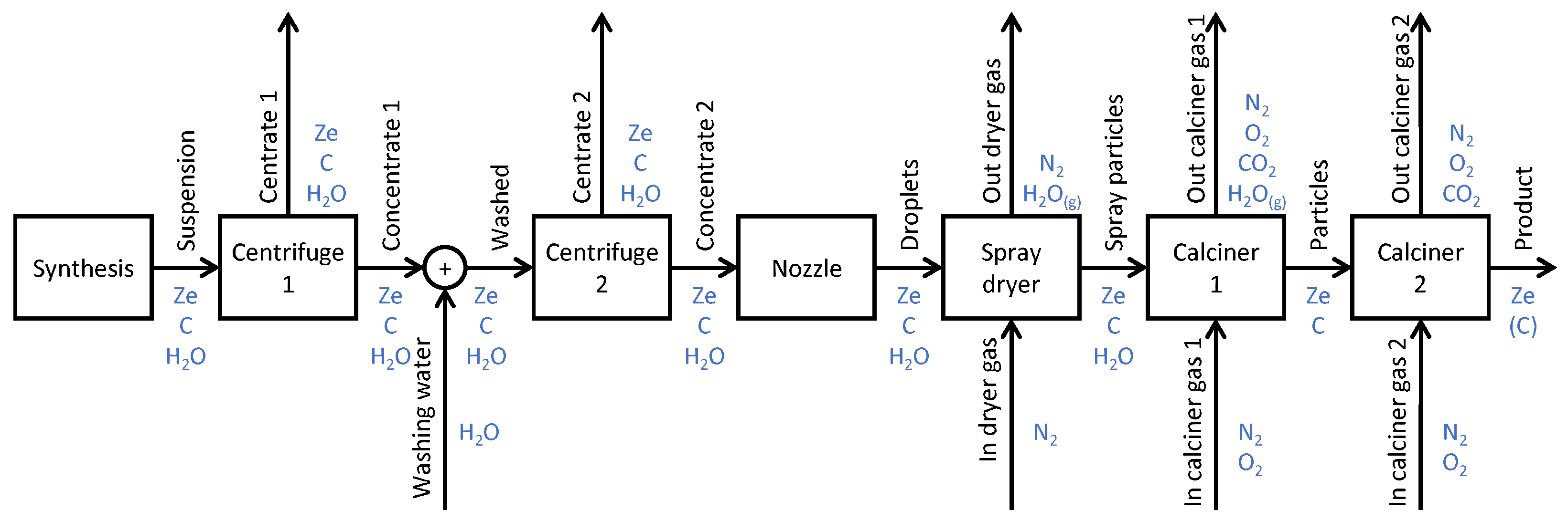
The flowsheet of the considered zeolite catalyst production process with corresponding material components is shown in
Figure 1. The catalyst particles (Ze) are formed due to agglomeration of precipitated reaction products within the synthesis unit operation. This unit is operated in batch mode. As the following processes are operated continuously, the synthesis step is calculated separately and its product is fed to the first centrifuge continuously. Between the two centrifugation stages, the slurry is washed with fresh water to remove hazardous byproducts from the concentrated slurry. The efficiency of the centrifuges depends strongly on the particle sizes of the zeolite products, which are in the range of nanometers. When the concentrated slurry enters the spray drying stage through a nozzle, the primary particles within the atomized suspension droplets agglomerate to larger particles in the micrometer range. Starting from the spray drying stage, the particle size grid is therefore adapted to larger product agglomerates. For the calcination, a rotary kiln with heated walls is used. In the first calcination stage, remaining water from the spray-dried particles evaporates. To avoid too high temperatures during the combustion of the organic residues, the first calcination stage is operated with a low oxygen concentration of the incoming gas. In the second calcination stage, the remaining organic residues are burned out of the product.
2.1. Synthesis
The zeolite synthesis process, taking place in the reactor, can be divided into several stages. In the beginning, the so-called unit cells are obtained from the initial reagents as a result of chemical transformations. These reactions can be mapped using fairly simple reaction kinetics. The emerged unit cells then precipitate, forming crystalline particles. An important final stage of the process is the agglomeration of the precipitated particles. This can be depicted using population balance models, parameterized with DEM simulations.
Since the real compounds, as well as some of their properties, cannot be disclosed for confidentiality reasons, the materials in the text are encrypted, and some of their parameters are changed.
2.1.1. General Model Structure
The influence of different process conditions on the synthesis is often difficult to predict since many parameters are interdependent. To facilitate this task, a multi-step strategy to develop a macroscale synthesis model suitable for flowsheet simulations is suggested. The general scheme of this approach is shown in
Figure 2. It comprises the following steps:
DEM is used to generate statistics on particle collisions for various values of process and material parameters;
Obtained information is used to find individual contributions of several empirical agglomeration kernels to the overall growth;
Found contributions and variations of process and material parameters are used to train a data-driven surrogate model of the agglomeration kernel;
The derived kernel is applied to build a PBM used in flowsheet simulations.
2.1.2. Microscale Model
DEM simulations with a variation of four process parameters were performed to extract statistics about the particles contact frequencies, needed to determine the agglomeration kernel. These are listed together with their limits in
Table 1. Latin hypercube sampling was utilized to generate a near-random set of parameter values in this 4-dimensional distribution. In total, 1200 samples with different combinations of parameters have been generated and simulated.
The Johnson–Kendall–Roberts (JKR) model [
40] was used to describe cohesive forces in particle–particle collisions. The corresponding equations are given in
Appendix A.1.1. To simulate the Brownian- and shear-induced particle motion in the liquid phase, the diffusion model of Depta et al. [
41] was adapted. Along with the temperature-dependent Brownian motion of particles, it allows defining a velocity profile for particles depending on their coordinates along the vertical axis (Z), thus enabling the simulation of particles shear. The model is described in
Appendix A.1.2.
To generate the initial scene, 50,000 particles were placed in a cubic volume with a side length of
, using an iterative force-biased algorithm [
42]. The generation volume was limited by periodic boundary conditions (PBC) on all sides, which made it possible to use such a small number of simulated objects (and, hence, to have acceptable simulation times), while maintaining the quantity and quality of obtained statistics. Given this number of particles and the size of the generation domain, the concentration of solids was significantly lower compared to the real process to simplify further contact detection and analysis.
Since the force-biased algorithm is used for the initial placement, the particles in the generated scene may have slight overlaps. They are usually very small (less then 1% of the radius) and therefore have no noticeable effect on the initial particle velocity. Yet, to avoid this effect completely, the sizes of all particles were artificially increased by 5% during generation, and then returned to their original size before starting the simulation. This allowed us to obtain the initial scenes without any particle intersections. The initial velocities of the particles were set equal to the corresponding flow velocities according to their Z coordinates (see
Appendix A.1.2).
In the real process, particles are agglomerated with a change in their size. Nevertheless, to reduce the computational effort, the diameters of the objects were kept constant during the simulation, so no actual particle fusion or breakage was modeled. Instead, only the contacts between particles, built due to cohesive forces, were analyzed. Therefore, the growth of granules was simulated indirectly, by introducing particles of different sizes into the simulation, which could collide, forming particles of other transitional diameters. By introducing particles of multiple sizes, it was possible to simulate a quasi-continuous grow of granules. In overall, the particles of 19 fixed sizes between and were modeled. Aggregates consisting of several particles make it difficult to collect statistics, so only binary ones were considered. Therefore, only a limited time interval could be meaningfully simulated before the particles form larger agglomerates of three or more objects. It was allowed only about 5% of objects to have non-binary contacts, otherwise, the statistics were considered unreliable. Thus, the total simulation time for each case was limited to . Given this restriction, each simulation was repeated three times, which was a compromise between simulation time and the amount of collision statistics collected.
The maximum allowed simulation time step was limited by the applied diffusion model [
41] and was equal to
where
is the density of particles,
is the minimum radius of particles on the scene, and
is the maximum fluid viscosity over all investigated case studies.
On the other hand, the critical simulation step for DEM is usually calculated in terms of the Rayleigh step
[
43], which depends on the particle size and the mechanical properties of the material, in particular, Young’s modulus and Poisson ratio. Usually, 10–20% of
is used as the simulation time step. With realistic values of mechanical properties of the modeled material, this evaluates to a critical step
which is quite small, causing long simulation times. Therefore, in order to speed up the computations, Young’s modulus
E of the particles was reduced to fit 20% of the critical time step for the diffusion model and back-calculated as:
where
is the Poisson ratio of particles. This made it possible to use a time step that, on the one hand, satisfies the limitations of the diffusion model, and, on the other hand, provides an acceptable duration of each simulation.
According to all these considerations, the following material and simulation parameters (
Table 2) have been applied for all DEM runs.
All DEM simulations were performed in the open-source framework MUSEN [
44], applying GPU-accelerated computations. The general view of the DEM scene at the end of the simulation with the particle velocity distribution is given in
Figure 3. The total CPU time spent to calculate all
simulations was about 670 days.
2.1.3. Data-Driven Model
Cohesive contacts between particles can continuously appear and disappear during the simulation. In order to select only those events that led to actual agglomeration, 3 time points were analyzed for each case: 0
,
and
, and the final contacts sets
C were calculated as
At first, all contacts that have arisen during the analyzed time interval of
were determined, and then those that were not long-term ones and disappeared at the end time point
were removed from the set.
To compensate for the effect of reduced density and different numbers of particles of each size, the number of contacts were further scaled by the number of particles as
where
is the number of contacts between particles of size
i and
j,
and
are the total number of those particles, respectively. In addition, due to the limited amount of data, they had to be further filtered to smooth out individual outliers.
The overall agglomeration behavior
was estimated as a composition of Brownian
and Shear
agglomeration kernels:
where
u and
v are particle volumes, and
,
, and
are size-independent agglomeration rate constants. The values of kernel coefficients
and
were estimated from the extracted collisions statistics using GlobalSearch optimization algorithm with fmincon solver from MATLAB. Thus, each sample of parameters in the range from
Table 1 was assigned two coefficients:
and
.
These values were used to train an artificial neural network model applying TensorFlow library [
45] used via Keras python interface [
46]. For each kernel coefficient, a separate multilayer perceptron with four inputs, one output, and several hidden dense layers has been created. To train the network, the Adam optimization algorithm [
47] with the mean squared error as the loss function was used. To design and set up the parameters of the model in an optimal way, KerasTuner hyperparameter optimization framework has been utilized with the validation loss as the objective function. It was allowed to change the following values: number of hidden layers (1 to 6), number of neurons (8 to 64), and activation functions (relu, sigmoid, softmax, tanh) for each layer, and the learning rate of Adam’s algorithm. The final obtained configurations were as shown in
Table 3. For both models, a learning rate of 0.01 was selected.
For the obtained ANN configurations, additional studies were carried out to determine the optimal number of training epochs, also using KerasTuner. They showed that the best number for Brownian and shear neural networks is 235 and 193, correspondingly. These settings were used to train the final models.
Before training the models, 10 outliers with a z-score greater than 2.7 were removed from the entire set of input data. For subsequent testing of the obtained models, 100 samples were excluded from the remaining ones, making up the test set. Additionally, to avoid overfitting, the cross-validation principle was used by splitting the available data set into validation and training subsets in proportion of 3:7. Thus, considering all of the above, the sizes of the sets were as follows:
Training set: 763 samples;
Validation set: 327 samples;
Testing set: 100 samples.
The final trained models were exported as a C++ module using the keras2cpp library [
48] for further integration within the flowsheet simulation framework Dyssol.
2.1.4. Macroscale Model
The obtained ANN were used as surrogate models, allowing easily linking process parameters and the agglomeration kernel. On their base, a macroscale population balance model was designed and implemented in the flowsheet simulator Dyssol as a batch unit.
The reaction model of the zeolite synthesis describes the transformation of initial reagents
,
, and
into unit cells
. The resulting unit cells precipitate in the form of X-ray amorphous particles, which in turn transform into crystalline particles. Thereafter, the crystalline particles are agglomerated until the final particle size is reached. Additionally, organic templates
are usually used [
10] to control the formation of the porous structure of the final product by providing a surface, where the nucleation process can start. In general, the reactions taking place in the apparatus can be described by the following simplified scheme:
where
is the stoichiometric coefficient of the corresponding reactant
i.
The time-dependent change in concentration of all materials is described as:
where
is the total volume of the solution,
is the number of formed X-ray amorphous particles per unit time, and
is the number of
moles per zeolite particle.
The kinetics of the first reaction (Equation (
9)) is calculated according to the Arrhenius equation, which leads to the following expression for the reaction rate:
Here,
denotes the reaction activation energy,
R is the universal gas constant,
T is the temperature,
is the dissolution constant for reaction 1,
is the molar concentration of
, and
is the fitting parameter. Experimental data on the compounds concentration were used to estimate the required kinetic parameters.
Based on the experimentally obtained concentrations, the rate of the second reaction (Equation (
10))—the formation of unit cells—was estimated as
Here, the values
are fitting parameters, and
is the pre-exponential factor of the second reaction.
The population balance of crystalline and X-ray amorphous particles describes the change in their numbers
N as:
The kinetics of the formation of X-ray amorphous particles and their transformation into crystalline particles are modelled using a self-accelerating kinetic approach, as shown in the equations:
where
and
are fitting coefficients.
To parametrize the concentration and number balances, experiments and resolved CFD simulations were used. Here, a laboratory-scale reactor with about 1.5 million cells, and a production-scale reactor with approximately 10 million cells were simulated in ANSYS Fluent. A polyhedral mesh with boundary layers and with mesh refinement at the locations with high shear rates was applied for both geometries. The calculations for the laboratory scale were laminar, transient, and used sliding mesh for the stirrer zone. For the production scale, calculations were performed stationary with the k-omega turbulence model and frame motion. For transient calculations, to ensure that the initial values do not influence the outcome, at least 10 revolutions of the stirrer were always simulated before the results were evaluated for one revolution.
In order to initiate the particle growth, all newly emerging crystalline particles (Equation (
21)) were assigned the size
, defined as a model parameter. The particle growth due to agglomeration is given by Equation (
22), where
is the agglomeration kernel, calculated with the previously described surrogate model, and
is the agglomeration rate constant. Fixed pivot technique [
49] was used to numerically solve Equation (
22).
It was found that the resulting model overpredicts the final particle sizes since it lacks an agglomeration stopping criterion. Further investigations are needed to establish the physics of this process. To overcome this shortcoming in the current implementation, the PBM model was extended with a size-dependent agglomeration rate coefficient
:
with fitting parameters
and
.
2.2. Decanter Centrifuge
After synthesis, the generated particulate matter is enriched by a solid–liquid separation step to achieve a sufficiently high solids content for the subsequent step of spray drying. In this case study, a continuously operating decanter centrifuge separates the synthesized solid material from the liquid phase. The physical principle of separation for this type of centrifuge lies in the existing density difference between the particulate solid and the continuous liquid phase. The main parts of a decanter centrifuge are a cylindrical-conical bowl, a screw conveyor, a feed pipe, an overflow weir, and a drive system (
Figure 4).
A pump conveys the slurry via the feed pipe into the machine. The decanter centrifuge works on the counter–current principle. This means that the slurry flows in the direction of the overflow weir and the conveyor system transports the formed sediment in the opposite direction. Due to the rotating bowl, the centrifugal force acts on the suspension and a pre-acceleration occurs at the transition between the cylindrical and conical parts of the decanter centrifuge. The centrifugal force acts on the slurry and forms the rotating liquid pond with the height of approximately the overflow weir. Solid particles have a higher density than the liquid and settle towards the inner wall of the bowl, forming a liquid-saturated sediment. Once the sediment is sufficiently compacted, the screw conveyor, which rotates with a small speed difference relative to the cylindrical-conical bowl, transports the material towards the conical part. Here, the sediment is ejected from the machine.
2.2.1. Model Structure
The dynamic model of the decanter centrifuge takes into account the sedimentation behavior, the sediment build-up of liquid-saturated bulk material with compressible behavior, and the sediment transport. The interconnection of individual ideally mixed compartments, as summarized in
Figure 5, forms the structure of the dynamic model.
The dynamic model divides the compartments into the sedimentation zone and the sediment zone. While the sedimentation zone represents the free flow of slurry in the machine, the sediment zone models the sediment build-up and transport. According to Menesklou et al. [
50], compartment interconnection of the sedimentation and the sediment zones allows us to predict process dynamics and the change in particle size distribution and solids content along the unrolled screw channel. Since this is a macroscopic modeling for use in the flowsheet simulation, assumptions and simplifications of the real process are necessary. A detailed discussion about the assumptions made can be found in Gleiss et al. [
33].
2.2.2. Model Equations
Sedimentation Zone
The stationary component balance for the relevant particle size considers the change of particle size distribution in each compartment
i:
Here,
and
are mass-related density distribution of particle size in the material flowing out of the compartment
i to the next sedimentation compartment and to the sediment compartment, respectively;
and
are the amount of particles of size
x flowing into and out of the compartment
i; and
is the amount of particles of size
x separated by centrifugal force. The change in total solids mass for each compartment is calculated as follows:
The accumulation term of the solids mass
depends on the incoming solids mass flow
, the outgoing solids mass flow
and the deposited solids mass flow
.
In order to solve the component balance of the solids phase, it is assumed that it is back-mixed in each compartment and the amount of separated solids can be described as a time-dependent separation efficiency,
The separation efficiency depends on the ratio of separated to incoming solid particles. Additionally, the integration of the feed density distribution and grade efficiency
T along the integration borders
and
allows us to calculate the separation efficiency in a compartment:
For direct calculation of the change in the volume fraction of solids in a compartment, the transformation of the unsteady mass balance (Equation (
25)) into a volume balance is carried out considering Equations (
26) and (
27):
where
is the volume fraction of the solid phase.
The grade efficiency, assuming a homogeneous distribution of particles over the entire flow cross-section, can be obtained from the geometric quantities, process settings and material properties as follows:
Here,
is the radius of the sediment surface,
is the radius of the overflow weir,
is the density difference between solid and liquid,
is the time-dependent hindered settling function,
x is the particle diameter,
is the dynamic viscosity of pure liquid,
is the angular velocity of the centrifuge bowl,
is the volume flow of the slurry,
is the screw pitch and
is the discretized length of the unrolled screw channel. At the beginning,
is equal to the bowl radius
. The hindered settling function is defined as:
where
,
,
, and
are model parameters.
The equations of the sedimentation zone apply only to the cylindrical part of the bowl.
Sediment Zone
The sediment zone includes the formation of sediment and the transport of liquid-saturated sediment towards the solids discharge. The transition between the sedimentation zone and the sediment zone is modeled by the gel point
. Analogous to the sedimentation zone, the solids mass balance can be established for the sediment zone:
Here,
is the accumulated solids mass in the sediment,
and
are the solids mass streams of transported material. The volume flow of the transportable sediment,
is the product of the volume-averaged solids volume fraction
in the sediment and the cross-sectional area
of the sediment, as well as the average transport velocity
. The cross-sectional area
of the sediment in the unrolled screw channel can be calculated from the side lengths
and
. Transforming mass conservation (Equation (
31)) to a volume balance and substituting Equation (
32) yields the final form of the equation to calculate the sediment transport in compartment
i:
The solids transport velocity depends on the the differential speed
between the screw and the bowl, the screw pitch angle
and the material behavior, which is described by the transport efficiency
k, and is given as follows:
The efficiency of the sediment transport is a crucial parameter, which depends on the material behavior as well as on the geometry of the screw and the process conditions. In the conical part, the cone angle leads to a decrease in the transport velocity, which is why Equation (
34) for the conical part must take into account the intersection angle
.
Additional geometric consideration are given in
Appendix A.2. In addition to the equations presented, models and material functions (e.g., settling behavior, sediment compression, shear compaction, transport efficiency) are required to calculate particle settling and sediment formation process and the volume of each compartment in the sedimentation zone. At this point, for a detailed description of the equation system for the dynamic model of the presented decanter centrifuge, the readers are referred to the already-published work [
32,
33,
34,
50].
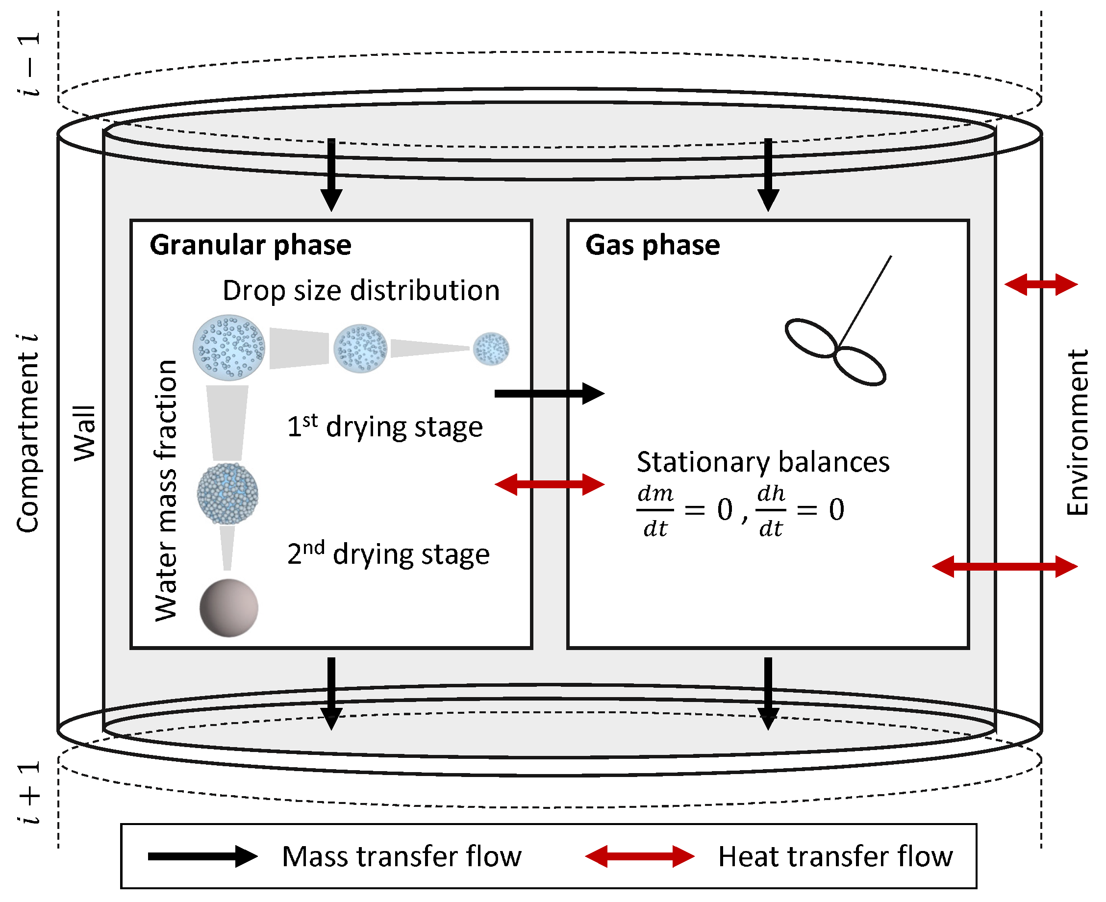
2.3. Spray Dryer
A multi-compartment approach is used to model the co–current spray drying process by discretization along the dryer’s vertical axis, according to the work of Buchholz et al. [
35]. The model structure is schematically shown in
Figure 6. In each dryer compartment, the suspension droplets before and after solidification are treated as a granular phase which is described by a two-dimensional population balance approach according to the particle size and water mass fraction. The model considers the heat and mass transfer between the gas and the particles, as well as the heat loss over the dryer wall. In each compartment, the respective phases are treated as ideally mixed. Due to negligible transient behavior, the system is modeled as quasi-stationary. The respective balance and constitutive equations are summarized in [
35].
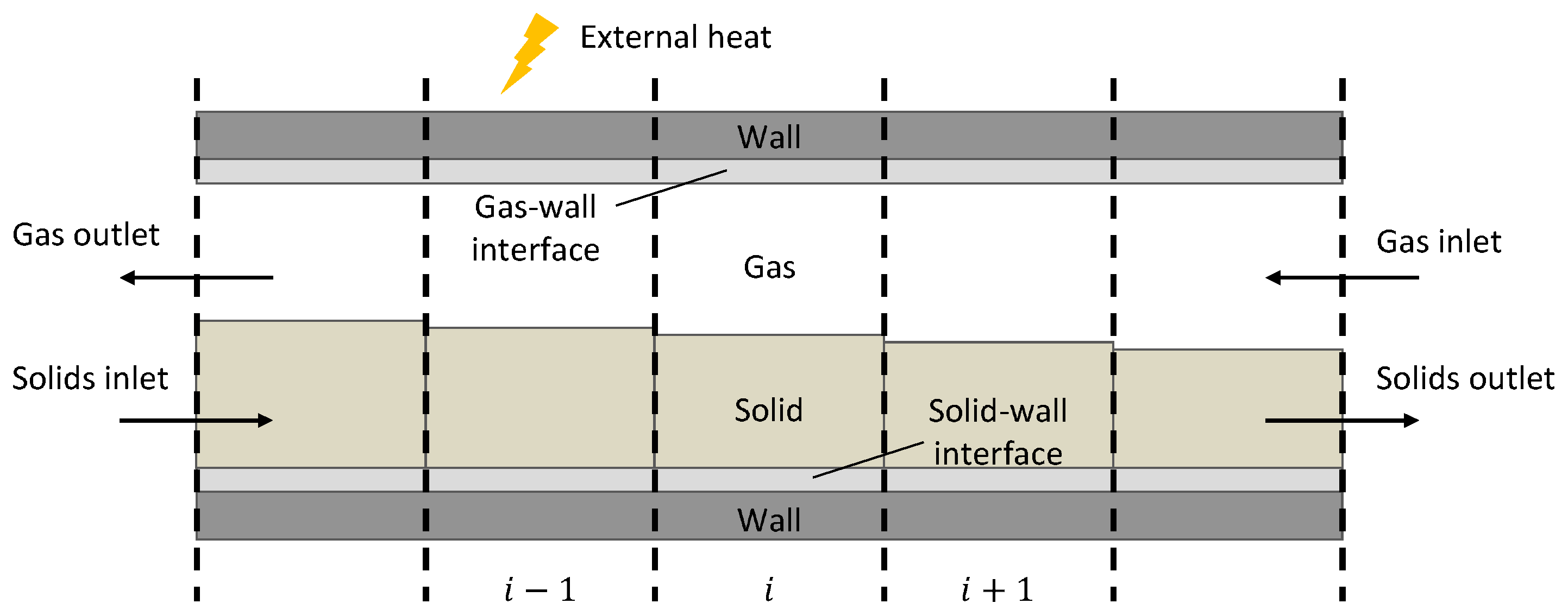
2.4. Rotary Kiln
The structure of the rotary kiln model is based on the works of Martins et al. [
51], Küssel [
36], and Ginsberg et al. [
52]. As shown in
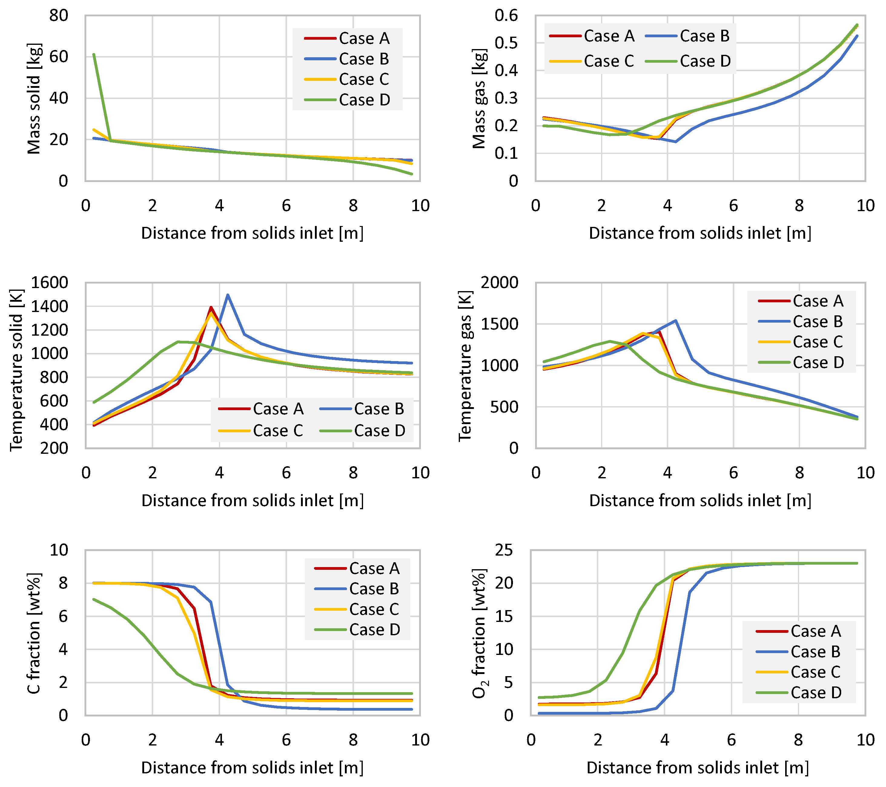
Figure 7, the kiln is divided along its horizontal axis into multiple compartments that consist of the following phases: gas (g), solid (s), and wall (w). Gas and solids move in opposite directions through the rotating kiln. The heat transfer between wall, solids, and gas phase is dominated by different heat transfer mechanisms which lead to a circumferential temperature profile in a thin layer of the inner kiln wall. Therefore, the inner part of the wall is divided into two distinct regions, i.e., a solid–wall (ws) and a gas–wall (wg) interface region. The kiln is externally heated on the outside of the wall to provide the energy needed to dry out the remaining water in the solid phase and to heat the substance to the temperature needed to start the exothermic combustion reaction.
In
Figure 8, the mass and heat flows between the different phases and regions are shown. The exchange mass flows between the solid and the gas phase in each compartment occur due to the evaporation of water and due to the combustion reaction. This leads to a mass flow of O
2 from gas to solid and a mass flow of the reaction product—in this case CO
2—from the solid to the gas phase. While the gas flows only in one direction, there is a backward-directed solids flow that accounts for possible back-mixing effects inside the particle bed. The amount of back-mixing and the overall particle velocity in the axial direction depend on the filling, the rotational speed, and possible internal structures inside the kiln. As the model does not describe this particle motion in detail, the information on the particle movement is taken from high-resolution CFD-DEM simulations of the whole kiln.
The heat transfer between the walls and solids is dominated by convection on the solid–wall interface due to the rotation. Additionally, the convective heat transfer between gas and solid and between gas and wall is described. The heat transfer via radiation is modeled between the gas–wall interface and the gas and the solid surfaces. Due to the rotation of the wall and the different temperatures of the respective wall interfaces, there is an enthalpy flow, also called regenerative heat transfer, between both wall regions. The external heat is conducted via the wall region towards the wall interface regions. Axial heat transfer is neglected.
In the following section, the mass and enthalpy balances that describe the phases of a single compartment are presented. The constitutive equations for the calculation of the heat and mass transfer are given in
Appendix A.3.
2.4.1. Solid Phase
In the solid phase, three compounds are present: an inert zeolite compound, an organic compound that is represented by pure carbon, and the remaining water after the drying process. The overall mass balance for the solid phase, which takes into account the forward and backward movement of the solid material as well as the mass exchange with the gas phase, reads as follows:
with subscript
r standing for reaction zone, and
denoting the number of reactions. The reaction terms of the solid phase
depend in this case on the reaction rate of the calcination reaction and the evaporation rate.
The general compound mass balance for compound
j is set up similarly to the overall mass balance:
The calcination reaction is described by a simplified approach to the combustion reaction of an organic material, which is represented by carbon, i.e., . The reaction is assumed to take place at the solid bed surface, such that the reaction rate depends mainly on the concentration of the reactants and the surface area.
The enthalpy balance takes into account the enthalpy transfer due to mass flows between compartments
, the reaction enthalpy
, as well as the heat transfer with the other phases
as follows:
The specific enthalpy of the reaction products
is evaluated at the mean temperature of the gas and the solid phase,
is a model parameter needed to calibrate the reaction rates according to measurements. Additionally, the reaction enthalpy
is divided between both the solid and the gas phases using the constant
, which defines the corresponding heat shares.
2.4.2. Gas Phase
The overall mass balance and the compound mass balance for an exemplary compound
j of the gas phase are given below:
Heat exchange between gas and wall as well as between gas and solids is modeled as a combination of radiative and convective heat. The corresponding enthalpy balance of the gas phase reads as
2.4.3. Wall
The enthalpy balances of the wall–solid and the wall–gas interfaces are listed below:
Here,
T is the temperature of the corresponding wall interfaces and
is the specific heat capacity of the wall.
2.5. Implementation Aspects
The size of the granular material varies significantly over the production process. Therefore, in order to limit the number of classes for each individual subprocess, different grids of distributed parameters were applied for the respective units. For the synthesis and the centrifuges, the grid size was in the nanometer range. During the spray drying process, the small primary particles agglomerated and formed larger particles with sizes in the micrometer range. Moreover, the spray dryer model additionally required the distribution of particles by moisture content. Specific grid parameters are given in the corresponding appendices.
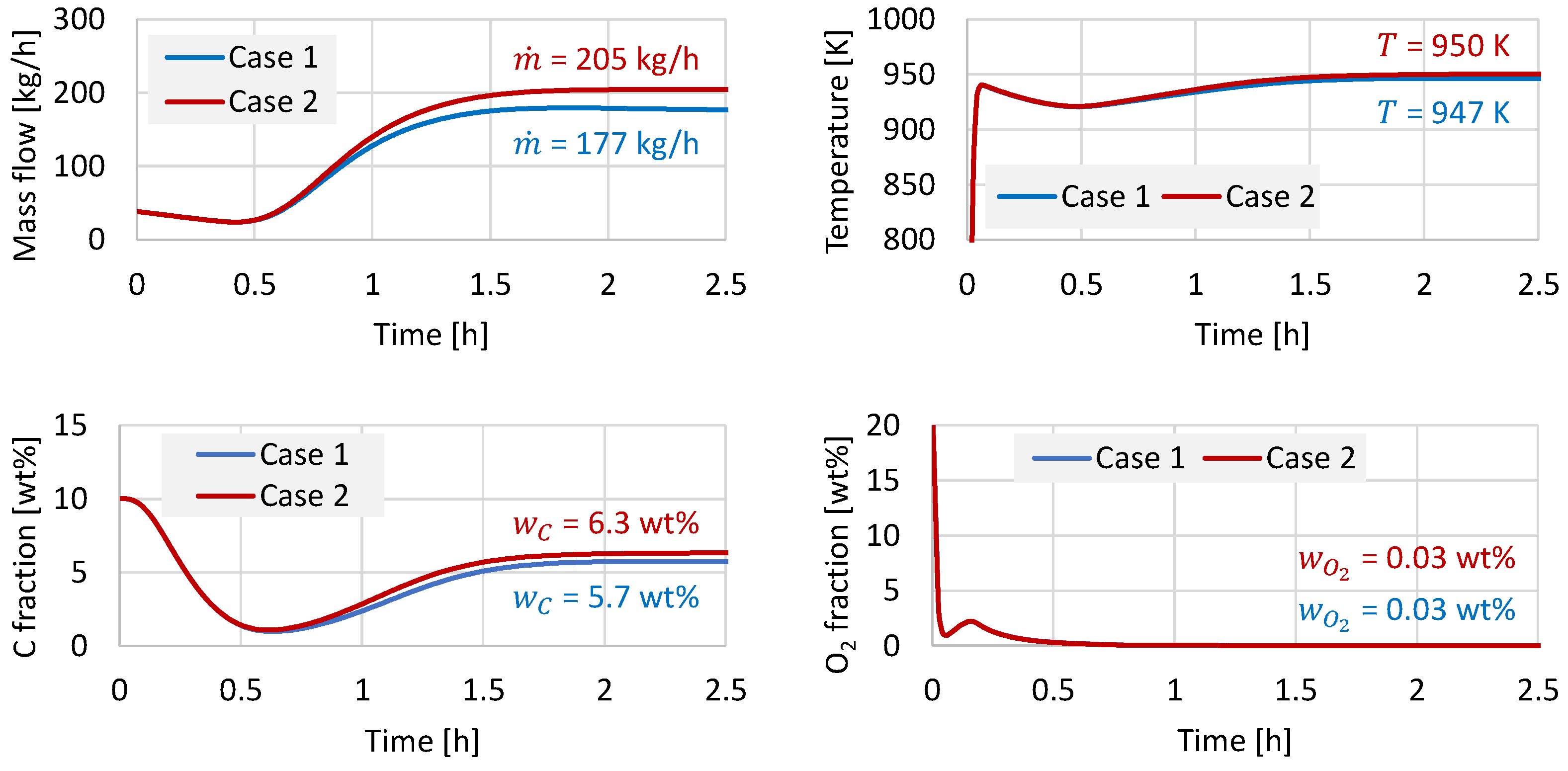
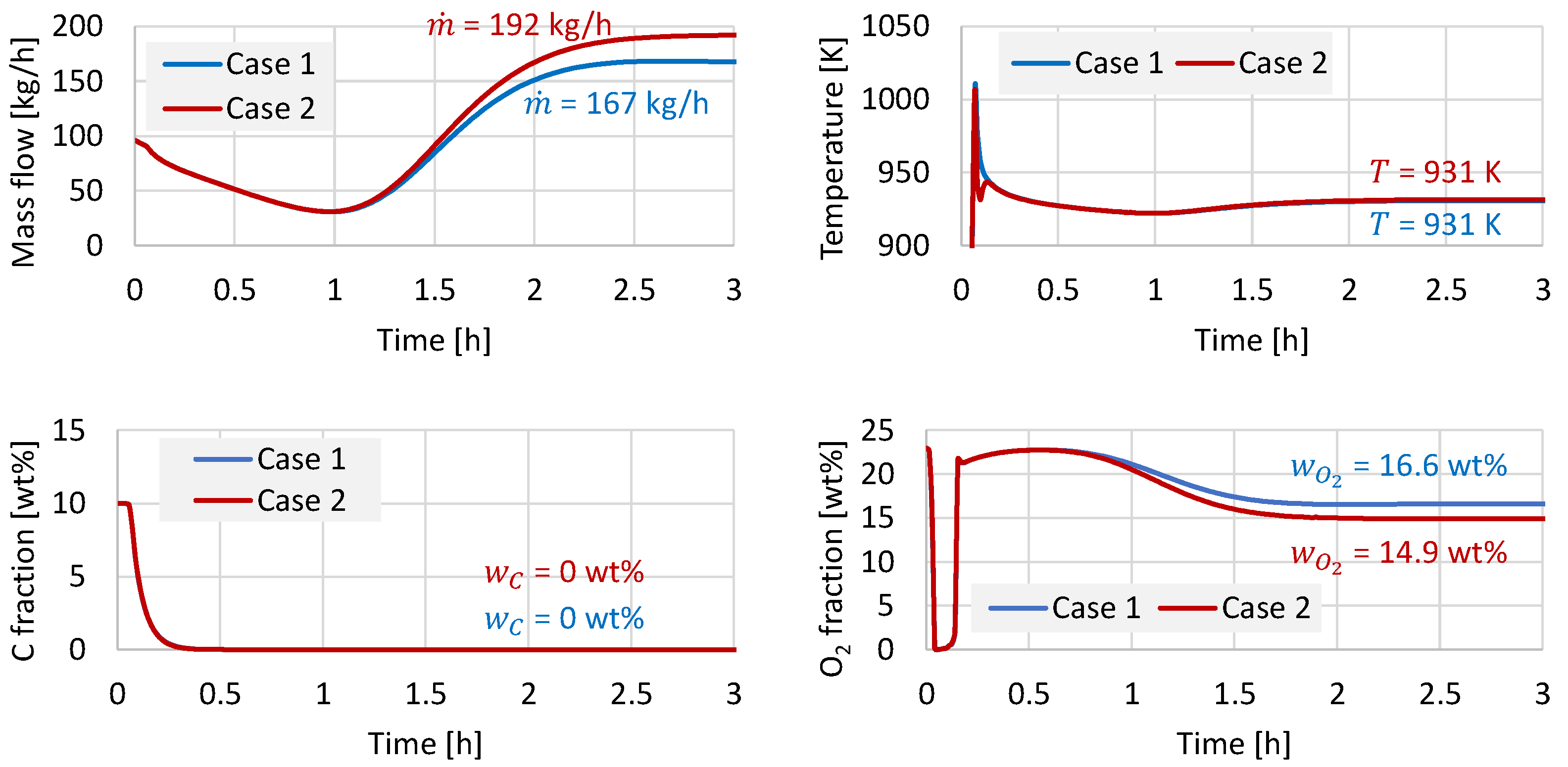
Another challenge is the connection of units operating in different modes. In particular, the synthesis reactor operates in a batch mode, so it was calculated in a separate flowsheet. Once it reached steady-state, the information about the final PSD was extracted and put as input to the solid–liquid separation process step, which was simulated with transient behavior. The following spray drying unit was described by a quasi-stationary model, which means that its calculations must converge at every time point. Therefore, to reduce the computational load, after the transient centrifugation process, the number of output time points was reduced to about 1 point per 10–100 .
4. Conclusions
This work proposes a framework for modeling the industrial process of zeolite production, consisting of four stages: precipitation and agglomeration in the synthesis reactor, liquid–solid separation in a decanter centrifuge, drying in a spray dryer, and calcination in a rotary kiln.
To develop the synthesis model, a novel multiscale and multistage approach is proposed. It is based on the description of the agglomeration process using a data-driven model. Discrete element modeling is used to generate data needed to derive a reliable surrogate representation of the agglomeration kernel. Information about collisions between different particles is extracted, analyzed, and used to train the artificial neural networks. The resulting surrogate model is able to describe the growth of particles due to agglomeration, correctly taking into account the mutual influence of various process parameters such as temperature, stirring speed, liquid viscosity, and particle surface energy. Based on this, a macroscale model operating in batch mode was designed, which can be used for flowsheet simulations.
The decanter centrifuge is described with a dynamic model, which takes into account the sedimentation process and sediment accumulation, as well as compression and transport of the resulting cake in the cylindrical and conical parts of the apparatus. Here, the multi-compartment principle is applied by dividing the entire length of the centrifuge into a series of compartments, each of which describes two ideally mixed zones: sedimentation and sediment.
The co–current spray drying process is modeled using a two-dimensional population balance approach that takes into account particle size and moisture content. The obtained quasi-stationary model describes heat and mass transfer between particles, gas, and the environment.
In the calcination stage, organic substances remaining after the synthesis are removed by combustion in a rotary kiln. In the developed multi-compartment model, it is possible to take into account the backward flow of the solid phase, which describes the possible effects of particle back-mixing. The gas moves in the direction opposite to the main flow of solids. The model is capable of describing chemical reactions at the gas–solid boundary, taking into account mass and energy balances between both phases and the kiln walls.
All obtained models were combined into a single flowsheet using the Dyssol modeling system, which allows simulation of the entire process of zeolite production. The developed framework made it possible to plausibly describe the production process, as well as to evaluate the mutual influence of various process parameters, operational conditions, and material properties on the processes occurring in each particular apparatus and, as a result, predict the properties of the final product. Moreover, the developed methods and models, as well as the entire flowsheet remain flexible, which means they can be further adjusted or fitted for use in other similar solids processes.


 ,
, 


