A Shift Schedule to Optimize Pure Electric Vehicles Based on RL Using Q-Learning and Opt LHD

Abstract

Range anxiety is a problem that restricts the development of pure electric vehicles. For this reason, much research starts from a shift schedule and strives to improve mileage. However, the proposed shift schedules have poor adaptive ability and are not suitable for dynamic conditions. In this paper, a shift schedule based on reinforcement learning (RL) is proposed, which uses Q-learning for optimization. However, the massive state variables and huge Q table in the state space put forward higher requirements on the computing power and storage space of the controller. Traditionally, the application of RL algorithms needs to rely on expensive GPU devices. To reduce high costs, we use an innovative treatment method, the optimal Latin hypercube design (Opt LHD), which is used for sampling, and state reduction is performed on the state space. Based on the above, the mileage is effectively improved by applying the shift schedule based on RL.

1. Introduction

The shift schedule affects the performance of the pure electric vehicle, such as power consumption economy and driving comfort. Research on shift schedule is conducive to further tapping the energy-saving potential of the pure electric vehicle, reducing the energy consumption and increasing the cruising range. Therefore, the study of the shift schedule plays an important role in pure electric vehicles.

J. Ruan et al. designed two customized shift schedules for DCT and CVT to improve economic performance [1]. Han K et al. proposed a collaborative optimization method for transmission design and shift schedule, which can effectively reduce energy consumption and improve the regenerative braking energy recovery efficiency [2]. Nguyen CT et al. developed an optimal shift schedule for acceleration and braking conditions based on a four-gear transmission with two motors. This shift schedule considers the motor efficiency and torque distribution, and also considers the influence of transmission ratio between different gears. Aiming at the hysteresis zone of the upshift and downshift curves, they developed a coordinated control strategy, which can achieve simultaneous upshift and downshift, effectively eliminating the shift interval and improving the shift quality [3]. To improve energy consumption, Kolmanovsky I et al. proposed a method for hierarchical optimization of the vehicle speed and shift schedule by using short-range traffic information flow. In this method, the integrated control problem is decomposed into pure continuous and discrete sub-problems, which overcomes the problem of calculating the integrated variable speed optimal control due to the different signal types of the vehicle speed signal and the gear signal [4]. Sujan VA et al. invented an adjustable shift schedule. The specific principle is to determine the loss power to overcome vehicle resistance according to the vehicle operation data. Based on the determined loss power, the vehicle operation parameters are optimized to compensate the loss of power. The shift schedule is dynamically adjusted to achieve the optimal shift and improve the adaptability to the dynamic unknown working conditions [5]. Jiang et al. used the volume Kalman filter estimation algorithm to accurately identify vehicle mass and road slope of the pure electric bus and use them as shift parameters. They proposed a four-parameter economical (EC) shift schedule considering vehicle speed, throttle opening, vehicle mass and road slope. The shift schedule not only considers the state of the vehicle itself, but also considers the influence of the vehicle mass change and the road slope on the driving gear, which further reduces the energy consumption of the vehicle, effectively avoids the frequent shift, and improves the riding comfort [6]. To integrate the power performance and economy of the vehicle, Huang et al. used the NSGA-II algorithm to conduct multi-objective optimization of transmission ratio of each gear, and solved the pareto optimal solution of the combination of transmission ratio. They designed a shift schedule based on dynamic programming (DP) with the goal of minimizing power consumption [7]. Sun et al. formulated a dynamic shift schedule according to the load characteristic diagram of the motor, which can significantly improve the working efficiency of the motor [8]. Lin et al. proposed a hybrid shift schedule for mechanical automatic transmission of pure electric city buses. By collecting and analyzing relevant data through bench test and real vehicle road test, the difference of driving conditions, shift characteristic points, and actual simplified transmission efficiency of urban routes are extracted. From the off-line global optimization results solved by DP algorithm, the comprehensive shift curve is extracted, and the typical features are fused together in a compatible way, so that it has better energy consumption performance under different working conditions in the city, and the universality of shift schedule is improved [9]. Qin et al. designed a shift schedule based on model predictive control. The changing trend of future working conditions is considered in the shift schedule, and the future vehicle speed change is predicted by neural network, and the trained neural network is used as the prediction model. Based on the optimal shift schedule designed by DP algorithm, and taking the shift schedule as the rolling optimization part of the model predicted shift schedule, the model predicted shift schedule was established. It not only saves energy consumption, but also reduces the shift frequency [10]. Li et al. proposed an algorithm to identify vehicle mass and road slope using the recursive least squares method, and based on this, designed a five-parameter shift schedule considering vehicle speed, acceleration, accelerator pedal (AP) opening, vehicle mass, and road slope. In addition to considering vehicle state and external environmental factors, the shift schedule also introduces the acceleration, which can reflect the dynamic performance of the vehicle, fully considers the driving intention of the driver, effectively improves the energy consumption performance, and realizes intelligent shift [11].

The research on the shift schedule of the pure electric vehicle mainly focuses on optimization, and a few shift schedules increase the shift parameters to improve the identification of the vehicle to the working condition, so that the ECU can make the optimal shift decision. The studies mentioned above improved vehicle performance. However, their essence does not get rid of the limitation of schedule-based shifts. Under the dynamic conditions, its energy consumption performance depends on the model prediction accuracy and identification accuracy. If the model is inaccurate or not accurate enough, the effect of shifting gears according to the shift schedule will be greatly reduced, which will inevitably lead to an increase in energy consumption.

Thus, this paper proposes a shift schedule based on RL to solve the problem of poor energy consumption under dynamic conditions. The principle of RL is that in an unknown environment, an agent can continuously improve its own behavior through continuous interaction with the external environment. The optimal control of the system can be realized by this operation, which is not limited by model accuracy and identification accuracy [12]. Although the RL using Q-learning can achieve the optimal learning effect, the massive state variables in the state space and the huge Q table put forward higher requirements on the computing power and storage space of the controller. Applications need to rely on expensive GPU devices, so the cost is high and the requirements are not met. Thus, the Opt LHD is used for sampling and state reduction is performed on the state space. Using Opt LHD sampling can reduce the number of tests, relieve the computational burden of the computer, and effectively reduce the computing power requirement on the premise of ensuring the uniformity and stability of the sampling.

The main research contents of this paper are as follows: The construction of the longitudinal dynamics model of the pure electric vehicle, the design of the EC shift schedule based on the vehicle speed and the AP opening, the design of the intelligent shift schedule based on RL, and the hardware of the pure electric vehicle in-loop simulation test. The remaining part of the paper is organized as follows. In Section 2, the vehicle dynamics model is built. Section 3 illustrates the design of the shift schedule based on RL. In Section 4, the in-loop simulation experiments are introduced. Finally, the conclusions are drawn in Section 5.

2. Modeling of the Pure Electric Vehicle

Modeling plays an important role in reducing R&D costs and improving development efficiency to build the pure electric vehicle model. The more accurate the model, the higher the reliability of the simulation experiment. The model of the pure electric vehicle includes the battery model, motor model, power train model, vehicle dynamics model, and driver model.

2.1. Driver Model

The driver model is mainly used to simulate the driver’s AP and brake pedal. The operating conditions are used as a reference, and the vehicle speed of the model simulation is used as a feedback. The AP opening and the brake pedal (BP) opening are the output in real time, and the driver model is based on PID control theory.

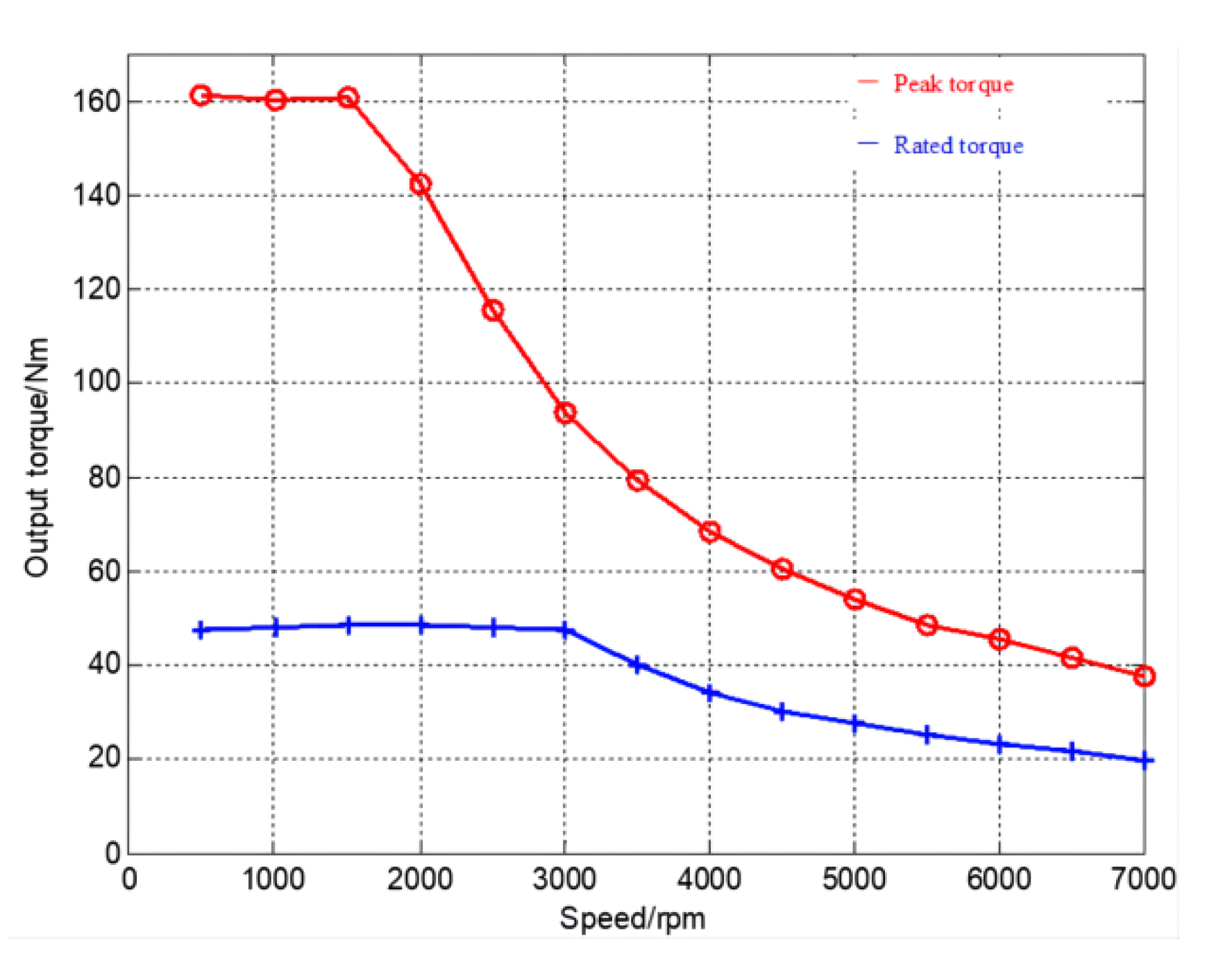
2.2. Motor Model

This paper adopts experimental data modeling [13]. The data modeling is based on the efficiency MAP of the motor and the external characteristic curves of the motor under different loads. In addition, the method of interpolation look-up table is used to determine the output of the motor under different working conditions. Figure 1 shows a MAP diagram of the motor efficiency. Figure 2 shows a graph of the motor speed and torque external characteristic curve.

In the modeling process, the input torque of the motor is related to the pedal opening. In general, the output torque of the motor has a linear relationship with the pedal opening, which is

$$T_{in}=f_1(\alpha ,n_m)$$

(1)

where $T_{in}$ denotes the output torque of the motor, and the unit is Nm; $\alpha$ is the AP opening, and the range is 0–1; $n_m$ is the meaning of the motor speed, and the unit is rpm; $f_1$ presents the torque interpolation function of the motor.

The input power of the motor can be expressed as

$$P_{in}=\frac{T_{in}{n}_m}{9550}$$

(2)

where $P_{in}$ is the input power of the motor, and the unit is kW.

In addition, because the motor has a certain power loss, its input power and output power are different. Moreover, the efficiency of the motor is different, and the degree of power loss is also different. The efficiency of the motor can be expressed as a function of the motor speed and motor torque, which is

$${\eta }_m=f_2(T_{in},n_m)$$

(3)

where ${\eta }_m$ denotes the efficiency of the motor; $f_2$ represents the efficiency interpolation function of the motor.

The output power of the motor is

$$P_{out}=P_{in}{\eta }_m$$

(4)

where $P_{out}$ is the output power of the motor, and the unit is kW.

When the vehicle is braking, the braking energy recovery of the motor also needs to be considered. Driving the motor can be regarded as doing negative work, which can be regarded as a process of charging the battery, and the tentative charging efficiency is 0.3.

2.3. Battery Model

This paper involves the study of the shift schedule of the pure electric vehicle, and the battery model considers parameters such as battery current, voltage, and SOC state estimation. Therefore, it is decided to use a relatively simple electrical model that is convenient for simulation analysis as a theoretical reference for modeling. Its equivalent circuit is shown in Figure 3.

According to Figure 3, the output voltage of the battery can be expressed as

$$U_{out}=U_0-IR$$

(5)

where $U_{out}$ denotes the output voltage of the battery, and the unit is V; $U_0$ is the voltage of the battery, and the unit is V; $I$ is the meaning of the output current of the battery pack; $R$ represents the internal resistance of the battery, and the unit is Ω.

The output power of the battery is the input power of the motor. Combined with the output voltage of the battery, the output current of the battery can be calculated as

$$\left\{\begin{array}{l}{P}_{out}=P_{in}\\ I=\frac{U_0-\sqrt{{U_0}^2-4R{P}_{in}}}{2R}\end{array}\right.$$

(6)

Assuming that the initial SOC value of the battery is 0.8, the SOC estimation of the battery adopts the ampere-hour integral method [14], which can be expressed as

$$SO{C}_{t+1}=SO{C}_t-\frac{I}{3600Q_0}$$

(7)

where $SO{C}_{t+1}$ is the meaning of the battery SOC in the next second, and the unit is %; $SO{C}_t$ represents the battery SOC at the current moment, and the unit is %; $t$ is the time, and the unit is s; $Q_0$ denotes the battery capacity, and the unit is AH.

2.4. Power Train Model

The motor involved in this paper is mechanically connected to the AMT without a clutch. Therefore, it can be considered that there is no loss in the process of torque transmission, and the output torque of the motor is the input torque of the power train. Therefore, the output torque of the power train can be expressed as

$$T_{trans}=T_{in}{i}_g{i}_0\eta$$

(8)

where $T_{trans}$ is the output torque of the transmission, and the unit is Nm; $i_g$ denotes the transmission ratio of each gear; $i_0$ is the meaning of the main reducer transmission ratio; $\eta$ represents the transmission efficiency of the AMT system.

The output speed can be expressed as

$$n_{trans}=\frac{n_m}{i_g{i}_0}$$

(9)

The gear selection and the transmission ratio of each gear are given by the shift schedule in the function module.

2.5. Vehicle Dynamics Model

The tractive force of the vehicle is

$$F_t=F_f+F_w+F_j+F_i$$

(10)

where $F_t$ denotes the traction required for driving; $F_f$ is the rolling resistance; $F_w$ is the meaning of the air resistance; $F_j$ represents the acceleration resistance; $F_i$ is the slope resistance.

The driving resistance, air resistance, acceleration resistance, and gradient resistance can be expressed as:

$$\left\{\begin{array}{l}{F}_f=mgf\\ F_w=\frac{C_{D}A{v}^2}{21.15}\\ F_j=\delta m\frac{dv}{dt}\\ F_i=mg\sin \theta \end{array}\right.$$

(11)

where $m$ denotes the vehicle mass, and the unit is kg; $g$ is the gravitational acceleration, and the unit is m/s²; $f$ is the meaning of the rolling resistance coefficient; $C_D$ represents the air drag coefficient; $A$ is the vehicle windward area, the unit is m²; $\delta$ represents the automobile rotating mass conversion factor; $\theta$ is the slope angle.

The true vehicle speed can be derived from the combination of Equations (11) and (12).

$$v={\displaystyle \int \frac{F_q-F_f-F_w-F_i}{\delta m}}dt$$

(12)

3. Design of Shift Schedules

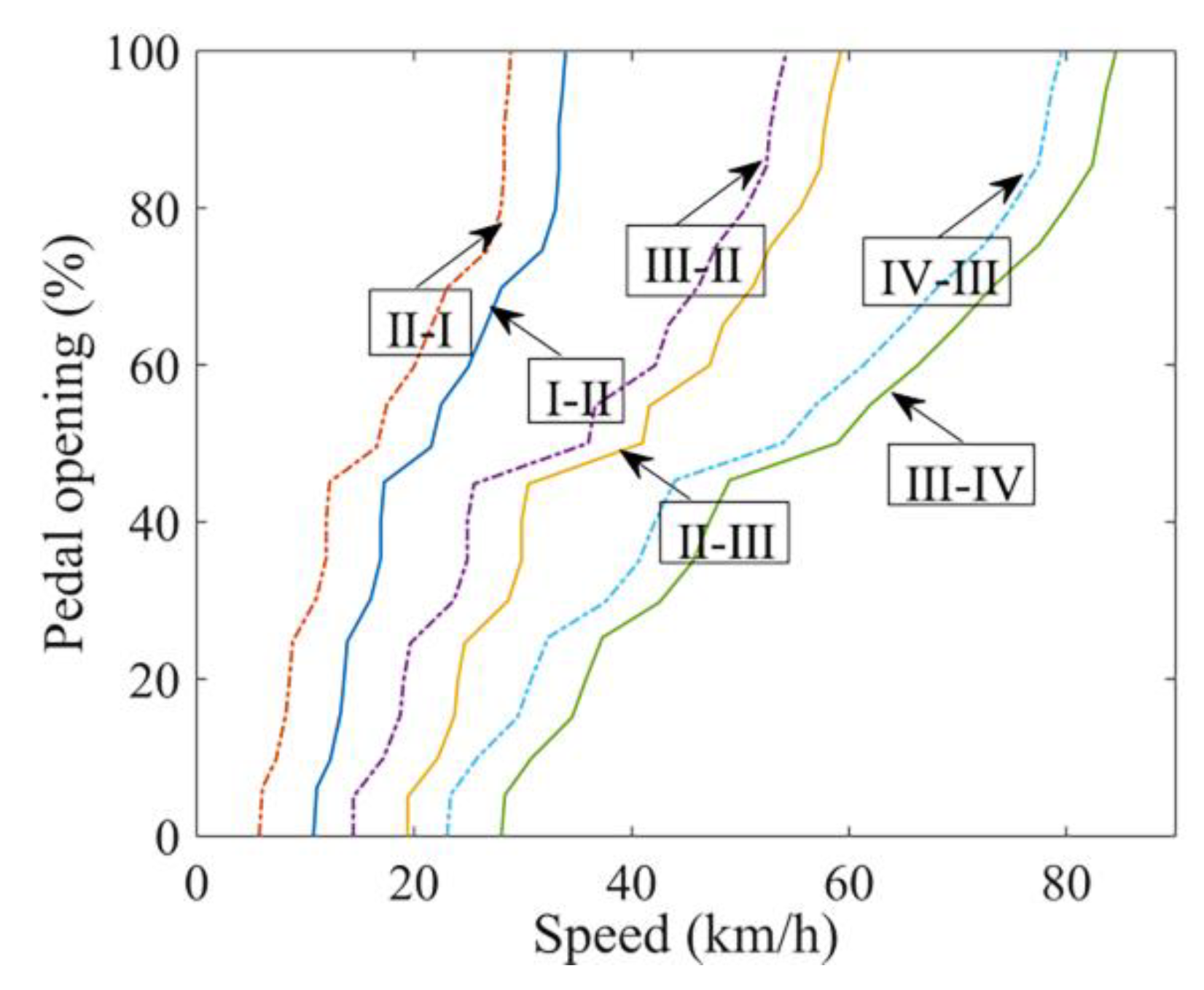
3.1. Design of EC Shift Schedule

The EC shift schedule is designed with economy as the goal, and the working efficiency of the motor is maintained in the high-efficiency region by selecting the appropriate shift point, so as to improve the driving range [15]. The current EC shift schedule control parameters generally use a pedal opening and vehicle speed. The design principle is to compare the working efficiency of the motor in different gears under the same pedal opening, and the efficiency intersection point of adjacent gears is the shift point at the pedal opening. The efficiency point is obtained as follows.

The relationship between the motor speed and the vehicle speed is

$$u=\frac{0.377n_{m}r}{i_g{i}_0}$$

(13)

Simultaneous Equations (1), (3), and (13) can obtain the relationship between motor efficiency and AP opening, vehicle speed, and transmission ratio.

$${\eta }_m=f_2(f_1(\alpha ,\frac{u{i}_g{i}_0}{0.377r}),\frac{u{i}_g{i}_0}{0.377r})$$

(14)

The efficiency surface of each gear is shown in Figure 4. The shift points of each gear are the points where the motor efficiency of the previous gear decreases and the motor efficiency of the next gear increases.

By changing the pedal opening within 0 and 1, the shift points at different openings can be extracted. To prevent the frequent shift problem caused by the pedal opening or vehicle speed near the shift point, 5 km/h is used as the shift speed difference. The EC shift schedule curve can be obtained, as shown in Figure 5. The six curves in the figure represent the downshift curve from 2nd gear to 1st gear, the upshift curve from 1st gear to 2nd gear, the downshift curve from 3rd gear to 2nd gear, the upshift curve from 2nd gear to 3rd gear, the downshift curve from 4th gear to 3rd gear, and the upshift curve from 3rd gear to 4th gear.

As can be seen from Figure 4, although the EC shift schedule meets the requirements of the long battery life, the motor efficiency at the shift point is low (about 80%).

3.2. Design of the Shift Schedule Based on RL

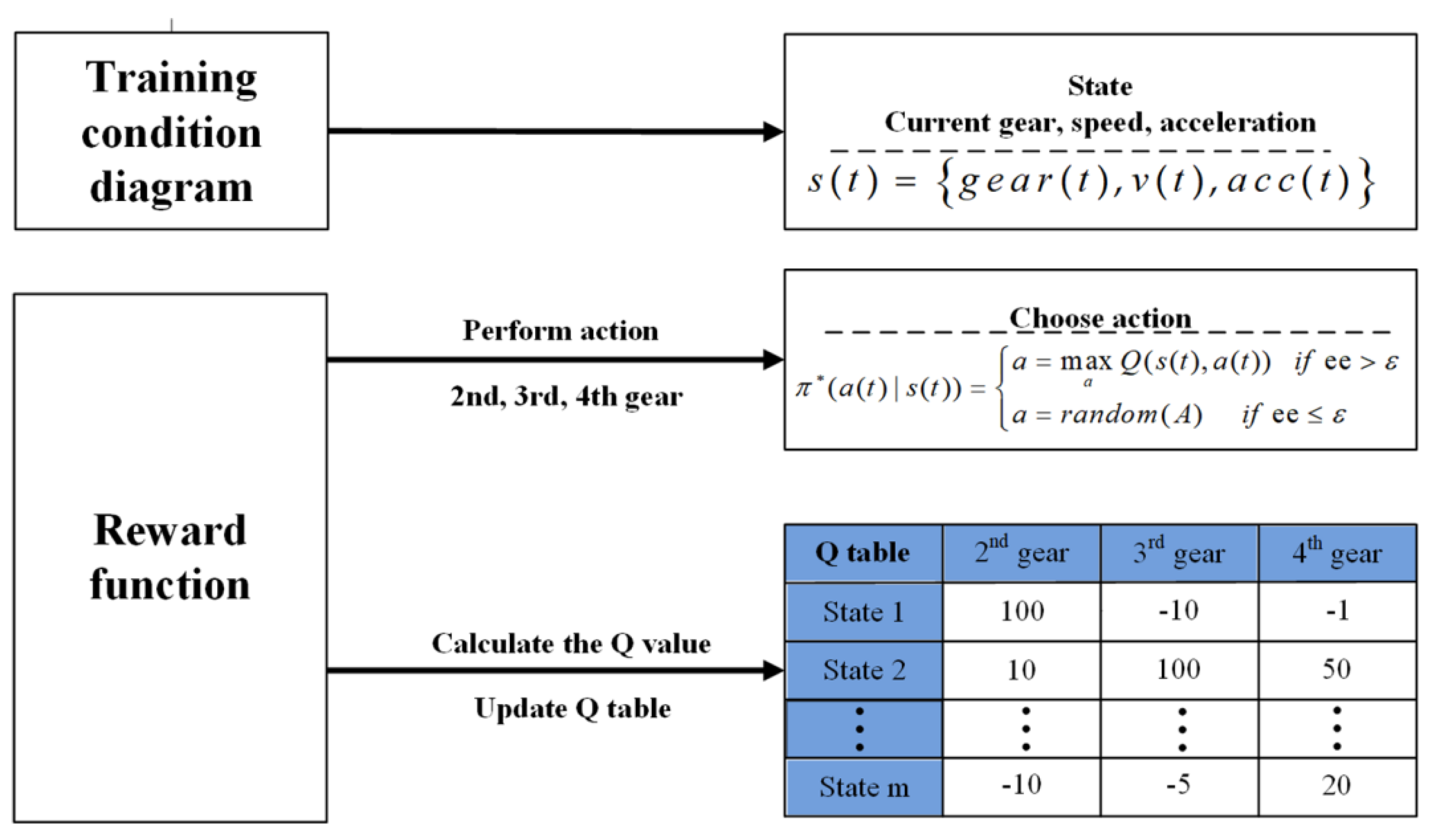
3.2.1. Establishment of States and Actions of RL Algorithms

Energy consumption is directly related to the efficiency of the motor, and the efficiency of the motor is directly related to its speed and torque. According to Equation (13), the motor speed is directly related to the vehicle speed. Therefore, the vehicle speed needs to be designed as one of the state variables. To describe the vehicle state finely and consider the representation of the state variables in the later stage, the vehicle speed range from 0 to 100 km/h is uniformly discretized into 99 specific states, which is

$$v(t)=\left[0,1.02,\dots ,100\right]$$

(15)

where $v(t)$ is the vehicle speed at time t.

Secondly, the motor speed is also related to the transmission ratio, so the current gear is also selected as a state variable. Since the research object is equipped with a 4-gear AMT, the first gear transmission ratio is extremely large, which is only used for large torque output, and is generally used for heavy loads and climbing. In normal driving conditions, the 2nd gear can be used to meet the needs. This paper does not consider the change of the slope and the mass of the vehicle, so it is decided to use three gears. The gear state can be described as

$$gear(t)=\left[2,3,4\right]$$

(16)

where $gear(t)$ is the gear at time t.

In addition, the energy consumption of the vehicle depends to a large extent on the proficiency of a person’s driving skills. In the absence of unexpected emergencies, frequent rapid acceleration or rapid deceleration will lead to poor energy efficiency. Therefore, the acceleration also needs to be designed as a state variable. According to the offline measurement of a large number of urban working conditions, the acceleration interval is taken as −2 to 2 m/s, and it is also uniformly discretized into 99 state points, which is

$$acc(t)=\left[-2,-1.96,\dots ,0,\dots ,1.96,2\right]$$

(17)

where $acc(t)$ is the acceleration at time t.

In summary, the state set can be expressed as

$$S=s(t)=\left[gear(t),v(t),acc(t)\right]$$

(18)

The state set $S$ can be expressed as a three-dimensional state space, and the number of states in the state space reaches 99 × 3 × 99 = 29,403.

To realize intelligent shift, the action of the RL is designed as the target gear, and it is designed as a discrete one-dimensional space; that is, the target gear is discrete in three points, which is

$$A=a\left(t\right)=\left[2,3,4\right]$$

(19)

where $a\left(t\right)$ represents the target gear at time t.

Each state variable in the state space corresponds to three different Q values. Therefore, the number of Q values in the Q table is 29,403 × 3 = 88,209. The state-action value function is stored by the Q table learned, and its state-action will be on the order of tens of thousands.

In addition, the Opt LHD sampling is adopted to reduce the state space.

3.2.2. RL State Space Reduction

When there is a lot of experimental data, Opt LHD sampling can reduce the number of experiments, relieve the computational burden of the computer, and effectively reduce the computing power requirement under the premise of ensuring the uniformity and stability of the sampling. To make the state variables of the shift schedule based on RL fill the entire state space as much as possible, this paper conducts sampling based on the idea of maximizing and minimizing distance. The specific steps are as follows: First, the scope of the state space is determined. Secondly, the minimum distance between each state variable and adjacent state variables is used as the characteristic distance, and the number of states in the state space after sampling is determined according to the requirements of the experimental design. Then, based on the number of states in the state space after sampling, the maximum distance between adjacent state variables is determined and sampled, so as to reduce the state space, and the maximum and minimum distance can be expressed as

$$\begin{array}{l}\underset{1\le i,j\le n,i\ne j}{\min }d(x_i,x_j)\\ d(x_i,x_j)=d_{ij}={\left[{\displaystyle \sum _{k=1}^m{\left|x_{ik}-x_{jk}\right|}^t}\right]}^{1/t}\end{array}$$

(20)

where $d(x_i,x_j)$ represents the distance between two sample points $(x_i,x_j)$.

The principle of determining the number of samples in this paper is to ensure the normal operation of the TCU, and the maximum number that can be programmed into the TCU shall prevail. The sampling results are shown in Figure 6.

Although the degree of refinement of the state description after sampling is reduced, the requirements for controller computing power and storage space are greatly reduced, and the uniformity and stability of sampling also ensure that the reduced state variables are representative.

3.2.3. Return Function of the Shift Schedule Based on RL

The reward function $R(s(t),a(t))$ in this paper is as follows

$$R(s(t),a(t))=\left\{\begin{array}{l}\frac{100}{Efficient\left(t\right)-efficient\left(t\right)}+\frac{1}{SO{C}_1\left(t\right)-SO{C}_2\left(t\right)},Efficient\left(t\right)-efficient\left(t\right)\ge 0.05\&\&SO{C}_1\left(t\right)>SO{C}_2\left(t\right);\\ \frac{100}{Efficient\left(t\right)-efficient\left(t\right)}+\frac{1}{SO{C}_1\left(k\right)-SO{C}_2\left(t\right)},Efficient\left(t\right)-efficient\left(t\right)\ge 0.05\&\&SO{C}_1\left(t\right)<SO{C}_2\left(t\right);\\ 1000\ast \left(Efficient\left(t\right)-efficient\left(t\right)\right)+\frac{1}{SO{C}_1\left(t\right)-SO{C}_2\left(t\right)},Efficient\left(t\right)>efficient\left(t\right)\&\&Efficient\left(t\right)-efficient\left(t\right)<0.05\&\&SO{C}_1\left(t\right)>SO{C}_2\left(t\right);\\ 1000\ast (Efficient\left(t\right)-efficient\left(t\right))+\frac{10}{SO{C}_2\left(t\right)-SO{C}_1\left(t\right)},Efficient\left(t\right)>efficient\left(t\right)\&\&Efficient\left(t\right)-efficient\left(t\right)<0.05\&\&SO{C}_1\left(t\right)<SO{C}_2\left(t\right);\\ 0,Efficient\left(t\right)=efficient\left(t\right)\&\&SO{C}_1\left(t\right)=SO{C}_2\left(t\right);\\ \frac{10}{SO{C}_1\left(t\right)-SO{C}_2\left(t\right)},Efficient\left(t\right)=efficient\left(t\right)\&\&SO{C}_1\left(t\right)>SO{C}_2\left(t\right);\\ \frac{10}{SO{C}_1\left(t\right)-SO{C}_2\left(t\right)},Efficient\left(t\right)=efficient\left(t\right)\&\&SO{C}_1\left(t\right)<SO{C}_2\left(t\right);\\ \frac{10}{Efficient\left(t\right)-efficient\left(t\right)}+\frac{1}{SO{C}_1\left(t\right)-SO{C}_2\left(t\right)},Efficient\left(t\right)<efficient\left(t\right)\&\&SO{C}_1\left(t\right)<SO{C}_2\left(t\right);\\ \frac{10}{Efficient\left(t\right)-efficient\left(t\right)}+\frac{1}{SO{C}_1\left(t\right)-SO{C}_2\left(t\right)},Efficient\left(t\right)<efficient\left(t\right)\&\&SO{C}_1\left(t\right)>SO{C}_2\left(t\right);\end{array}\right.$$

(21)

where $Efficient(t)$ denotes the efficiency of the motor after shifting at time t; $efficient(t)$ is the meaning of the motor efficiency that keeps the original gear at time t; $SO{C}_1(t)$ is the battery SOC after shifting at time t; $SO{C}_2(t)$ represents the battery SOC of the original gear and is maintained at time t.

From Figure 5, it can be seen that the difference between the efficiency at the motor shift point and the maximum efficiency of the motor is about 15%. Under the premise of considering the economy and taking into account the shift frequency at the same time, after many tests, the efficiency difference is finally designed to be 5%.

3.2.4. Establishment of the Shift Schedule Based on RL

In this paper, the action set is designed as the target gear, so the RL algorithms of Q-learning are mainly used to find the best target gear. Therefore, under each time step, the optimal control strategy ${\pi }^{\ast }(s(t),a(t))$ can be expressed as

$${\pi }^{\ast }(s(t))=\arg \underset{a_t}{\max } Q(s(t),a(t))$$

(22)

where $Q(s(t),a(t))$ is the meaning of the Q value to perform the action $a(t)$ in the current state $s(t)$. In this paper, the optimal Q value is defined as

$$Q^{\ast }(s(t),a(t))=R(s(t),a(t))+\gamma \underset{a^t\in A}{\max } Q^{\ast }(s^{\prime }(t),a^{\prime }(t))$$

(23)

where $R(s(t),a(t))$ is the meaning of the reward obtained after performing the current action $a(t)$; $\gamma$ denotes the discount factor, $\gamma \in \left[0,1\right]$; $\underset{a^t\in A}{\max }{Q}^{\ast }(s^{\prime }(t),a^{\prime }(t))$ represents the maximum value of all actions at the next moment corresponding to the Q table in the next state $s^{\prime }(t)$.

Furthermore, the update of the Q table can be expressed as

$$Q(s(t),a(t))=Q(s(t),a(t))+\alpha •(R(s(t),a(t))+\gamma \underset{a^t}{\max } Q(s^{\prime }(t),a^{\prime }(t))-Q(s(t),a(t)))$$

(24)

where $\alpha$ is the recession factor, $\alpha \in \left[0,1\right]$.

This paper adopts the more common strategy $\epsilon -greedy$ in RL to select actions. To put it simply, strategy $\epsilon -greedy$ is a regulation strategy for the tendency of an agent to choose two optimization methods when choosing an action [16], which can be specifically expressed as

$${\pi }^{\ast }(a(t)|s(t))=\left\{\begin{array}{ll}a=random(A)& if \mathrm{ee}\le \epsilon \\ a=\underset{a}{\max } Q(s(t),a(t))& if \mathrm{ee}>\epsilon \end{array}\right.$$

(25)

where $\epsilon$ is the random exploration probability, $\mathrm{ee}$ is the meaning of the random number, and the unit is [0~1].

In the early stages of offline training, to improve the learning efficiency, $\epsilon$ takes a larger value, so that the optimization method is more inclined to random exploration, so as to find as many better actions as possible. With the continuous progress of offline training, the value of $\epsilon$ gradually decreases, so that the optimization method gradually tends to the optimal method of the Q table until the Q table converges. The offline training process of the Q table is shown in Figure 7.

At each step, the RL agent determines the current state with the current gear, acceleration, and vehicle speed. Next, select the corresponding action based on the $\epsilon -greedy$ strategy and execute it to obtain the reward value in the current state. Then, calculate the Q value under the current action and update the Q table according to the reward value and the historical cumulative reward. Finally, the next state is updated based on the state parameters such as the current gear, and the above steps are repeated to update the Q value under the next state and action until the training ends, and the Q table is derived.

The purpose of offline training is to ensure that the vehicle can drive in the most economical gear in different states as much as possible. Therefore, the working conditions of the offline training should cover the entire state space as much as possible to ensure that the vehicle can drive in the optimal gear in any state. In this paper, four sets of internationally recognized test conditions are used to train the Q meter offline. The four groups of working conditions are the urban working condition WVUCITY for low-speed driving, the suburban working condition WVUSUB for medium-speed driving, the high-speed working condition HWFET for high-speed driving, and the mixed working condition UDDS [17]. The main eigenvalues are shown in

Table 1. Characteristic values of each working condition.

Working Condition	Time	Distance	vmax	amax
WVUCITY	1408 s	5.29 km	57.65 km/h	1.14 m/s2
WVUSUB	1665 s	24.81 km	72.10 km/h	1.30 m/s2
HWFET	766 s	16.41 km	96.40 km/h	1.43 m/s2
UDDS	1370 s	11.99 km	91.25 km/h	1.48 m/s2

.

It can be seen from Table 1 that the four groups of operating conditions almost cover the state of the full speed section. Therefore, using four sets of working conditions as training conditions can ensure that the coverage of the state space can reach the expectation.

Figure 8, Figure 9, Figure 10 and Figure 11 shows the results obtained by training the four groups of working conditions in the order of urban working conditions → suburban working conditions → high-speed working conditions → mixed working conditions.

In Figure 8a, for the front and rear of the WVUCITY condition, the vehicle speed is generally lower. In the middle section, there are several violent accelerations and decelerations, and the vehicle speed is high. Therefore, in Figure 8b, the front and rear are mostly driven in 2nd/3rd gear, and sometimes it is raised to 4th gear in the middle. However, due to the large change in vehicle speed at this stage, the gear is not maintained for a long time. The urban training Q table is taken as a reference, the suburban working conditions are trained, and the results are shown in Figure 9. In Figure 9a, at around 200 s, there are two periods when the vehicle speed exceeds 50 km/h in the WVUSUB condition. The gear in Figure 9b is also raised to 4th gear. However, at 400~600 s, according to the operating condition information in Figure 9a, when the vehicle speed exceeds 50 km/h, it does not shift to 4th gear. It may be because the corresponding state point is not collected when Opt LHD is used for sampling, so that in this state, the AMT selects the operation to maintain the original gear.

The results of continuing to train the high-speed case are shown in Figure 10. Under high-speed conditions, the frequency of shift is significantly reduced because the vehicle runs at a high speed throughout the entire journey, and there is almost no rapid acceleration or rapid deceleration.

After the training of the first three working conditions, as shown in Figure 11, it is the training result under the mixed working conditions. It can be found that although the vehicle speed fluctuation is relatively severe, the real-time performance of the gear is better in the low, medium, and high speed stages.

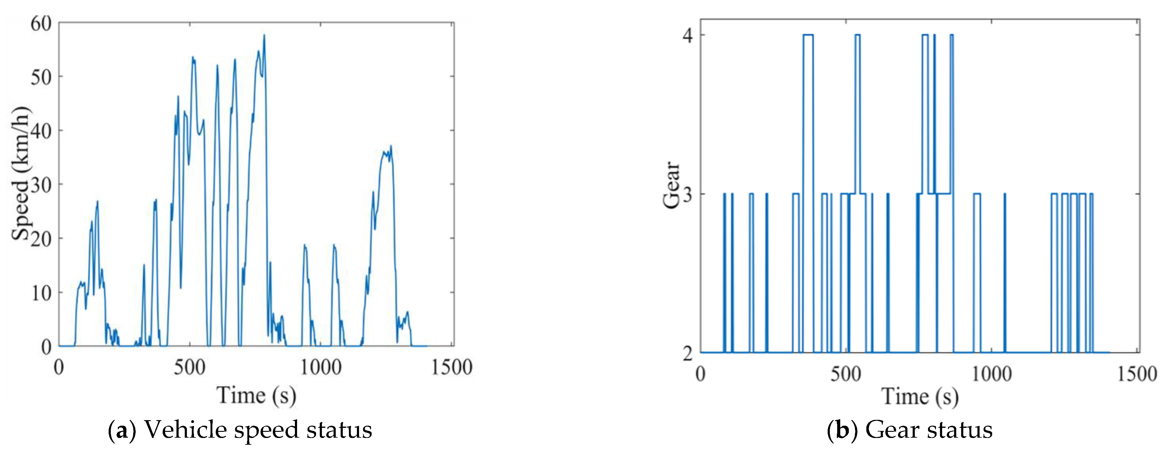
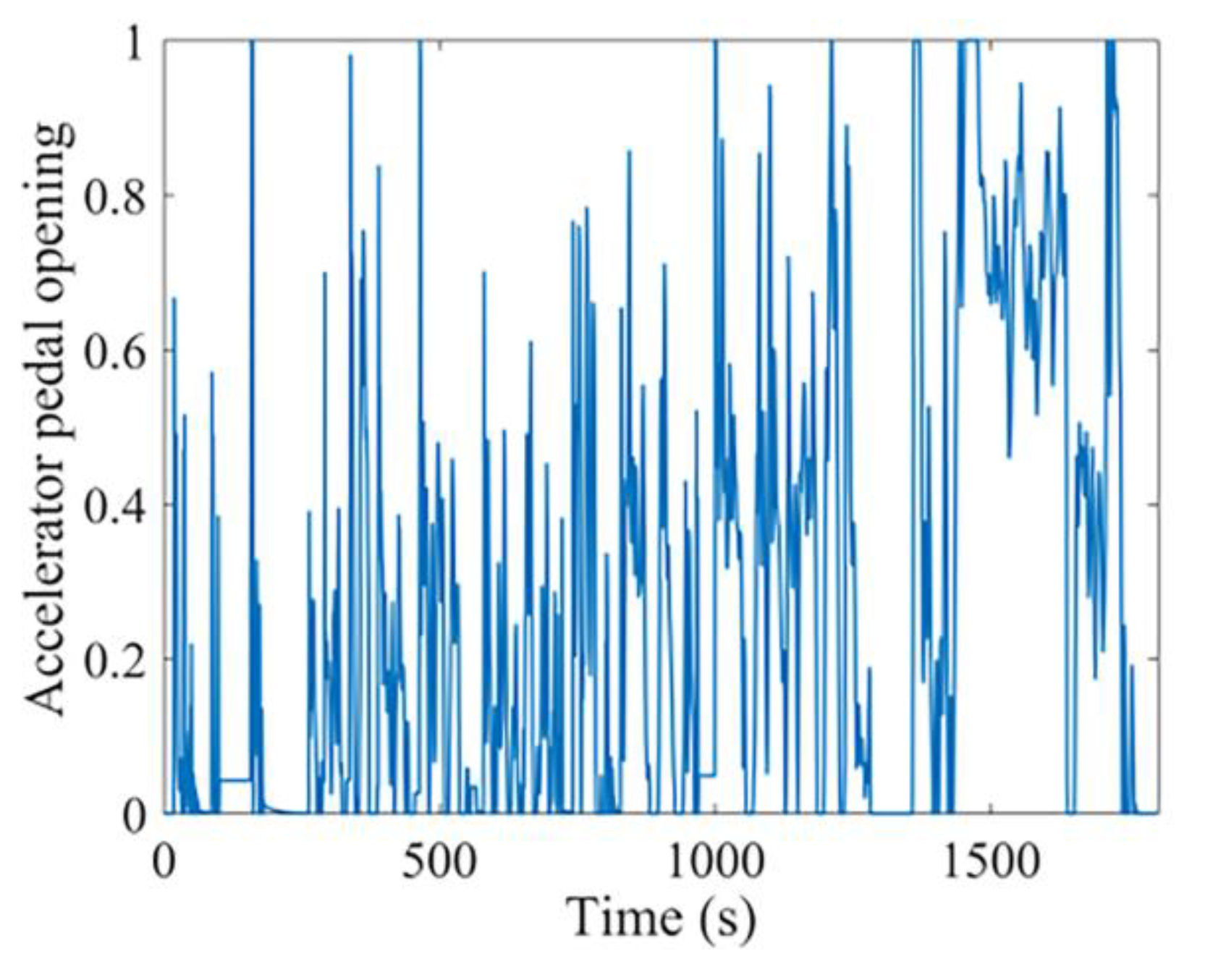
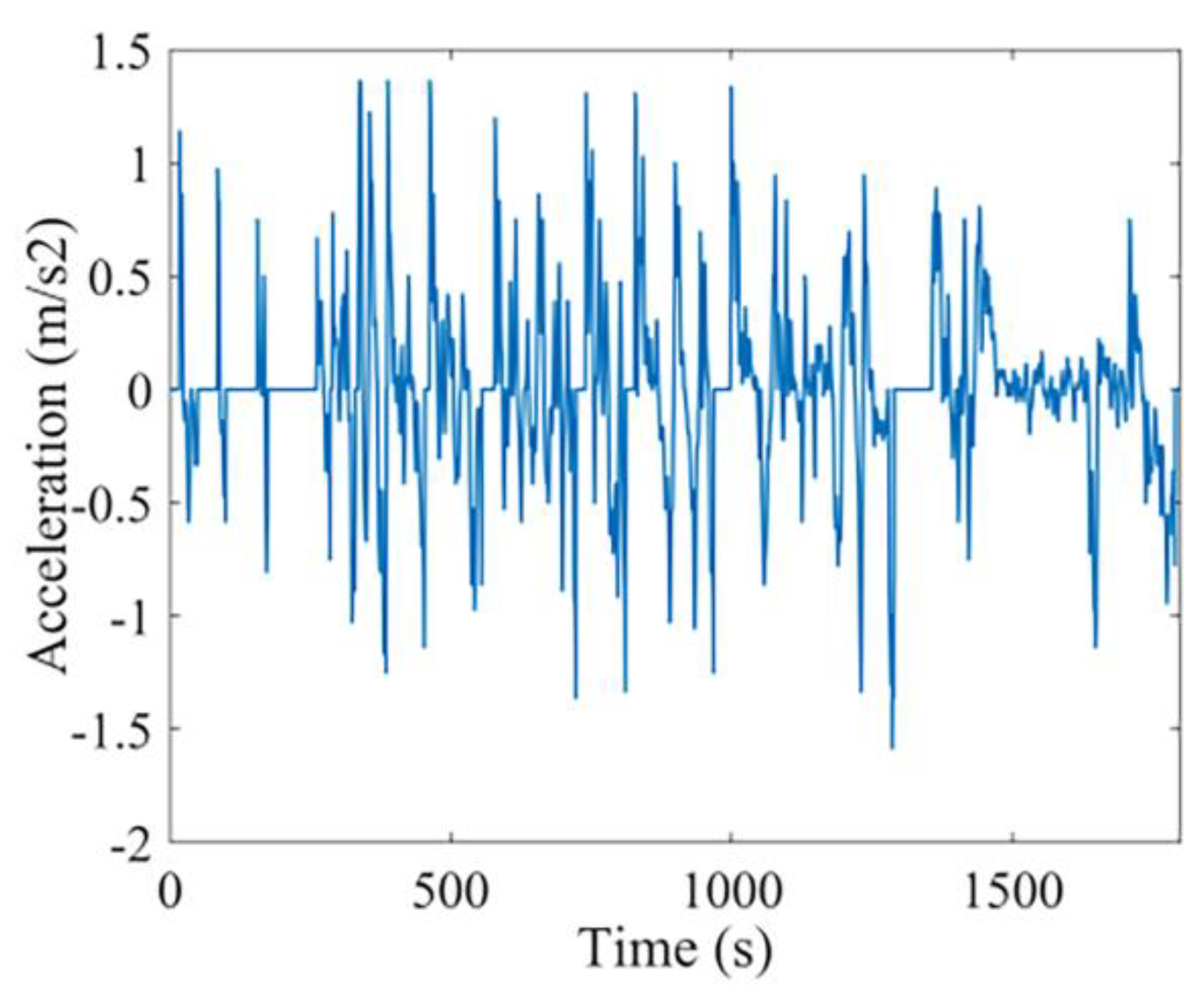
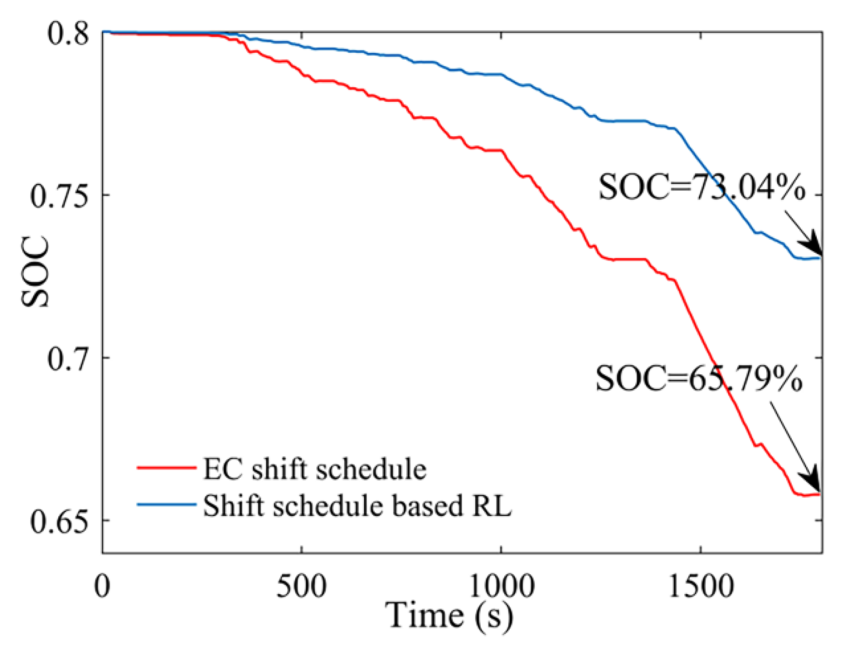
3.2.5. Model Simulation Verification

To test the performance of the shift schedule based on RL in terms of energy consumption economy, the next step is to conduct software-in-the-loop simulation tests for two shift schedules based on the pure electric vehicle model. Considering the usage scenarios and uses of the research object, it was decided to adopt the China light vehicle test cycle (CLTC) specified in the national standard of the People’s Republic of China as the test condition [18]. The CLTC is shown in Figure 12.

The CLTC working condition information is taken as the expected vehicle speed. After it is given to the driver model, the output AP opening is shown in Figure 13, and the acceleration and vehicle speed following output by the driving model are shown in Figure 14 and Figure 15 respectively.

As can be seen from Figure 13, due to the rapid fluctuation of operating conditions, the change of the AP opening is also more frequent. Figure 14 also proves that there will be rapid acceleration during driving. The pedal opening will appear to be deeply depressed to ensure the power of the vehicle. It can be seen from Figure 15 that the actual vehicle speed can follow the target vehicle speed well, which further ensures the reliability and accuracy of the subsequent simulation. Based on the above working condition information, the two shift schedules are brought into the vehicle model for simulation [19]. The gear comparison diagram is shown in Figure 16, and the SOC result comparison diagram is shown in Figure 17.

Combined with the simulation conditions, it can be seen from Figure 16 that in the low-speed road section, the vehicle speed is generally low, and the vehicle is driven in a low gear under the EC shift schedule. The shift schedule based on RL adopts shifting gears to deal with the change of working conditions. This is due to the change of the state of the vehicle resulting in the change of the optimal gear, which shows that the shift schedule based on RL has a certain adaptability [20]. In the medium-speed section, due to the severe fluctuation of working conditions, frequent shift occurs under the EC shift schedule, while the problem of frequent shift does not occur under the shift schedule based on RL, which also proves the rationality of the design of return function in the previous paper. In the high-speed road section, due to the sudden deceleration in the second half of the high-speed working condition, the shift schedule based on RL and the EC shift schedule are adopted to change the gear position. Combining with Figure 17, it can be seen that both of them have different degrees of braking energy recovery, which is in line with practical applications. At the same time, the whole cycle is about 16.4 km in length. In terms of data, under the EC shift schedule, the SOC remains 65.79%. Under the shift schedule based on RL, the SOC remains 73.04%, and the energy consumption is reduced by about 7.27%.

On the whole, shift schedule based on RL can effectively reduce the energy consumption of the pure electric vehicle and improve the cruising range.

4. Hardware-in-the-Loop Experiment

4.1. Introduction to Hardware-in-the-Loop Platforms

The pure electric vehicle performance comprehensive test platform takes PXI as the core, and integrates six hardware modules: Driving simulator (Modified version based on cs75 console, Chang’an Automobile, Chongqing, China), battery pack (RiseSun MGL, Beijing, China), wheel speed simulator, motor, AMT (self-development) and chassis dynamometer. The human-computer interaction platform developed based on LabVIEW and the virtual environment built based on CarSim together constitute the software system of the hardware-in-the-loop experimental platform [21]. The experimental platform architecture is shown in Figure 18.

The platform is mainly divided into three parts, which are the host computer, the lower computer and the underlying actuator. The host computer is the PC side of the computer and runs the human-computer interaction software written by LabVIEW. The communication function between the PC and PXI is realized through the local area network to ensure the real-time transmission and display of data. In addition, the virtual environment built based on CarSim is also displayed and runs on the PC side. The lower computer is PXI, which realizes the signal interaction with the underlying actuator through CAN communication, and feeds back the signal of the underlying actuator to the host computer. The longitudinal dynamics model of the vehicle runs in the lower computer.

The underlying actuator mainly uses the AMT’s gear selection motor and drive motor. According to the obtained vehicle status signal, the TCU judges the target gear, coordinates and controls the response of the motor and the gear selection motor, and then realizes the switching of gears. The TCU feeds back real-time signals to the lower computer through CAN communication, and the host computer reads the real-time data fed back to the lower computer by the underlying actuator through the local area network to realize the closed-loop simulation of the system. In addition, driving simulators, battery packs, wheel speed simulators, and chassis dynamometers can also be considered as categories of underlying actuator. The driving simulator is used to output the AP/BP opening signal and the shift handle position signal. The power battery pack provides power for the entire hardware-in-the-loop test platform, and feeds back the SOC to the host computer in real time. The wheel speed simulator is used to simulate the wheel speed. The chassis dynamometers are used to simulate the driving resistance of the car during driving.

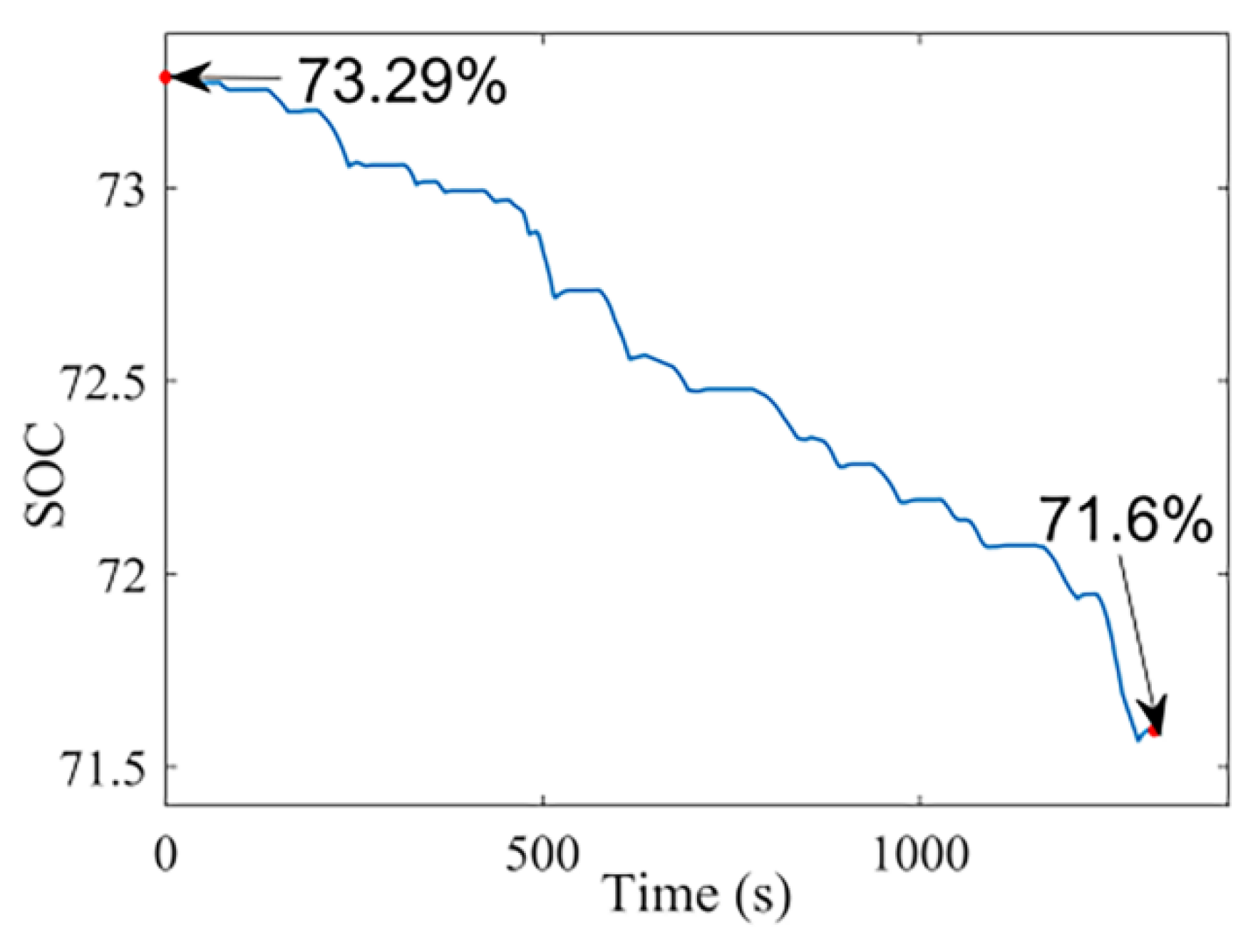
4.2. Hardware-in-the-loop Experiments and Analysis

Dynamic Shift Experiment

This section compares and verifies the two shift schedules through dynamic shift experiments.

To ensure the consistency of the experimental conditions and eliminate the interference of human factors on the experimental results as much as possible, this paper conducts experiments based on fixed operating conditions, and comprehensively considers the application scenarios of vehicles mainly in China. Therefore, the experiment is carried out using China Typica, a typical domestic working condition. The China Typica working condition is shown in Figure 19.

In this test, the driver model running on the lower computer outputs the AP/BP opening, and the driving simulator is only used to realize the position control of the shift handle.

Figure 20, Figure 21, Figure 22, Figure 23, Figure 24 and Figure 25 show the experimental results of the EC shift schedule based on the hardware-in-the-loop platform and the experimental results of the shift schedule based on RL. The two state parameters of the EC shift schedule are vehicle speed and pedal opening. When the hardware in the loop platform is tested, the working condition is read by the host computer software and directly sent to the driver model of the lower computer for operation.

As shown in Figure 20, the change of the pedal opening is in line with the changing trend of the working conditions. There is good feedback in the rapid acceleration and rapid deceleration segments, indicating that the output parameters of the driver model are accurate and real-time.

The reliable driver model ensures the smooth progress of the dynamic shift schedule experiment, and its gear map and SOC change map are shown in Figure 21 and Figure 22. In the low-speed section, although the vehicle speed fluctuates violently, the two state parameters do not reach the shift threshold, the AMT does not shift under the EC shift schedule. In the medium-speed section, when the vehicle speed exceeds 30 km/h, the AP opening exceeds at 50%, and the AMT will shift to the 3rd gear. Only when the vehicle speed exceeds 50 km/h and the AP opening exceeds 70%, the AMT will shift to the 4th gear. There were only three times of driving in 4th gear during the whole journey, and in high probability cases, they were all in low gears and driving with a large AP opening. Figure 22 reflects the SOC change under the EC shift schedule. The SOC change under this condition is 4.87%. The acceleration is calculated comprehensively based on the virtual load dynamically imposed by the chassis dynamometer, and the output is shown in Figure 23. It can be seen from the figure that the acceleration varies between −1 and 1 m/s. At the same time, the acceleration shows an instantaneous sudden change and short-term maintenance. The comparative analysis shows that this is also consistent with the characteristics of rapid acceleration and rapid deceleration under the China Typica working condition, which can reflect the state change of the vehicle to a certain extent.

Figure 24 reflects the gear map under the shift schedule based on RL. It is not difficult to see that the shift frequency is significantly increased compared with the EC shift schedule, and the frequency of switching back and forth between 2nd/3rd gear is mostly increased. This is because the Q table that stores the reinforcement learning shift rule defines the optimal gear in each vehicle state based on the motor efficiency. By analyzing the China Typica working condition, it is not difficult to find that the vehicle speed in this working condition mostly fluctuates between 0 and 40 km/h, and switching between 2nd/3rd gear is a normal phenomenon. In addition, in the range of 1200~1300 s, there is a maximum vehicle speed (60 km/h) under this working condition, but during the experiment, it did not increase to 4th gear in this state. Through the collected vehicle state parameters, the state of the vehicle is not found by searching the Q table. The reason for this situation is that the Opt LHD sampling results in the reduction of state variables, so when the vehicle reaches this state, the operation of maintaining the original gear is adopted by default.

The shift schedule based on RL designed in this paper is based on economy. The SOC change map as shown in Figure 25. The change of SOC is 1.69%. Compared with the EC shift schedule, the energy consumption is reduced by about 3.18%, which proves the feasibility and application potential of the shift schedule based on RL.

Experiment results of the EC shift schedule:

Figure 20. Pedal opening.

Figure 20. Pedal opening.

Figure 21. Gear of the EC shift schedule.

Figure 21. Gear of the EC shift schedule.

Figure 22. SOC of EC shift schedule.

Figure 22. SOC of EC shift schedule.

Experiment results of the shift schedule based on RL:

Figure 23. Acceleration.

Figure 23. Acceleration.

Figure 24. Gear of the shift schedule based on RL.

Figure 24. Gear of the shift schedule based on RL.

Figure 25. SOC of the shift schedule based on RL.

Figure 25. SOC of the shift schedule based on RL.

5. Conclusions

In this paper, a multi-speed AMT pure electric vehicle is taken as the research object, and a shift schedule based on RL is proposed to improve vehicle energy performance. The main conclusions are as listed as follows:

(1)

The proposed shift schedule can continuously self-learn according to the reward and punishment mechanism designed by the reward function and match the best gear according to the principle of economy. It solves the problem of high energy consumption caused by poor adaptability of traditional shift schedules.

(2)

The Opt LHD was introduced to reduce the state space of the Q table of the shift schedule, and solved the problem that the shift schedule could not be embedded in the TCU due to the “dimension disaster”. Using Opt LHD sampling can reduce the number of trials, ease the computational burden of the computer, and effectively reduce the computing power demand.

(3)

Compared with the EC shift schedule, energy consumption is reduced by about 3.18% by using the shift schedule based on RL. The feasibility and application potential of the shift schedule based on RL have been proven.

Overall, the method proposed in this paper taps the energy economy potential of multi-speed pure electric vehicles. The shift schedule based on RL proposed in this paper provides a new case for the combination of machine learning and shift schedule, and also provides a new idea for reducing the energy consumption of electric vehicles. Researchers can use other machine learning methods to optimize the shift schedule, which is not limited to RL. However, the proposed method has some shortcomings. First of all, due to the consideration of the impact of shift frequency on ride comfort, the design of the reward function is not based on the highest efficiency, but is designed in the form of a difference. Although shift frequency is reduced, energy consumption has been improved. Secondly, due to the problem of controller computing power, the state space of the Q table should not be too large. Therefore, the number of state variables is limited, and the accuracy of the Q table to describe the vehicle state needs to be further improved. In the future, through continuous research, the above problems will be solved.

References

- Ruan, J.; Walker, P.; Zhang, N. A comparative study energy consumption and costs of battery electric vehicle transmissions. Appl. Energy 2016, 165, 119–134. [Google Scholar] [CrossRef] [Green Version]
- Han, K.; Wang, Y.; Filev, D.; Dai, E.; Kolmanovsky, I.; Girard, A. Optimized design of multi-speed transmissions for battery electric vehicles. In Proceedings of the 2019 American Control Conference (ACC), Philadelphia, PA, USA, 10–12 July 2019; pp. 816–821. [Google Scholar]
- Nguyen, C.T.; Walker, P.D.; Zhang, N. Optimization and coordinated control of gear shift and mode transition for a dual-motor electric vehicle. Mech. Syst. Signal Process. 2021, 158, 107731. [Google Scholar] [CrossRef]
- Han, K.; Li, N.; Kolmanovsky, I.; Girard, A.; Wang, Y.; Filev, D.; Dai, E. Hierarchical optimization of speed and gearshift control for battery electric vehicles using preview information. In Proceedings of the 2020 American Control Conference (ACC), Denver, CO, USA, 1–3 July; 2020; pp. 4913–4919. [Google Scholar]
- Sujan, V.A. System and Methods of Adjusting a Transmission Shift Schedule. U.S. Patent 9,989,147, 5 June 2018. [Google Scholar]
- Yuanguang, J.; Haonan, L.; Jiankun, P.; Zhanjiang, L. Research of the AMT Multi Parameter Fusion Shift Rule of Pure Electric Bus. Mech. Transm. 2019, 43, 21–26. [Google Scholar] [CrossRef]
- Huang, W.; Huang, J.; Yin, C. Optimal design and control of a two-speed planetary gear automatic transmission for electric vehicle. Appl. Sci. 2020, 10, 6612. [Google Scholar] [CrossRef]
- Sun, G.B.; Chiu, Y.J.; Lu, G.W.; Xiong, M. The Study of Dynamic Programming with Fuzzy Logic Energy Design and Simulation of Gear Shift for Electric Vehicles. J. Netw. Intell. 2019, 4, 88–99. [Google Scholar]
- Lin, C.; Zhao, M.; Pan, H.; Yi, J. Blending gear shift strategy design and comparison study for a battery electric city bus with AMT. Energy 2019, 185, 1–14. [Google Scholar] [CrossRef]
- Hang, Q.; Hongwen, H.; Mo, H. Electric Vehicle Shift Strategy Based on Model Predictive Control. J. Chongqing Univ. Technol. 2021, 35, 90–95. [Google Scholar]
- Li, H.; He, H.; Peng, J.; Li, Z. Five-parameter shift strategy of automatic mechanical transmission for electric bus. DEStech Trans. Env. Energ. Earth Sci. 2019. [CrossRef]
- Li, G.; Görges, D. Ecological adaptive cruise control for vehicles with step-gear transmission based on RL. IEEE Trans. Intell. Transp. Syst. 2019, 21, 4895–4905. [Google Scholar] [CrossRef]
- Wenguang, L.; Shanshan, B.; Chang, X. Shifting Strategy for Two-Speed AMT of Electric Vehicle. J. Chongqing Univ. Technol. 2021, 35, 41–49. [Google Scholar]
- Liu, Z.; Li, Z.; Zhang, J.; Su, L.; Ge, H. Accurate and efficient estimation of lithium-ion battery state of charge with alternate adaptive extended Kalman filter and ampere-hour counting methods. Energies 2019, 12, 757. [Google Scholar] [CrossRef] [Green Version]
- Zhu, B.; Zhang, N.; Walker, P.; Zhou, X.; Zhan, W.; Wei, Y.; Ke, N. Gear shift schedule design for multi-speed pure electric vehicles. Proc. Inst. Mech. Eng. Part D J. Automob. Eng. 2015, 229, 70–82. [Google Scholar] [CrossRef]
- Samadi, E.; Badri, A.; Ebrahimpour, R. Decentralized multi-agent based energy management of microgrid using RL. Int. J. Electr. Power Energy Syst. 2020, 122, 106211. [Google Scholar] [CrossRef]
- Yi, J.; Li, X.; Xiao, M.; Xu, J.; Zhang, L. Construction of nested maximin designs based on successive local enumeration and modified novel global harmony search algorithm. Eng. Optim. 2017, 49, 161–180. [Google Scholar] [CrossRef]
- Chen, J.; Su, Y. Fuel Consumption and Nox Emissions from Vehicle Over the Wltc and Cltc_C. Available online: https://ssrn.com/abstract=4046059 (accessed on 17 October 2022).
- Powell, B.K.; Bailey, K.E.; Cikanek, S.R. Dynamic modeling and control of hybrid electric vehicle powertrain systems. IEEE Control. Syst. Mag. 1998, 18, 17–33. [Google Scholar]
- Lewis, F.L.; Vrabie, D. RL and adaptive dynamic programming for feedback control. IEEE Circuits Syst. Mag. 2009, 9, 32–50. [Google Scholar] [CrossRef]
- Sun, Y.; Ru, Y.; He, X.; Dong, C. Research on Testing System and Test Method for Charging Facilities of Electric Vehicles. In Proceedings of the 2018 5th IEEE International Conference on Cloud Computing and Intelligence Systems (CCIS), Nanjing, China, 23–25 November 2018; pp. 1048–1052. [Google Scholar]