WSN-Based SHM Optimisation Algorithm for Civil Engineering Structures

Abstract

With the development of economy and the improvement of architectural aesthetics, civil structure buildings show a trend of diversification and complexity, which brings great challenges to the Structural Health Monitoring (SHM) of civil structure buildings. In order to optimise the structural health monitoring effect of civil structures, reduce monitoring costs, and improve the ability of civil structures to deal with risks, a civil structure health monitoring method combining Variational Modal Decomposition (VMD) and the Gated Recurrent Unit (GRU) is proposed. The gated neural network algorithm of modal decomposition is used, and then a wireless sensor network (WSN) civil structure health monitoring model is constructed on this basis. Finally, the application effect of the model is tested and analysed. The results show that the network energy consumption of this model can reach a minimum of 0.05 J, which is 0.05 J less than that of the Gate Recurrent Unit (GRU) model. The minimum loss value is 0.08. Its Mean Absolute Error (MAE), Root-Mean-Square Error (RMSE), and Mean Absolute Percent Error (MAPE) are 0.03, 0.04, and 0.06, respectively; the prediction error is the smallest, the overall amplitude difference monitored by the model remains at a low level of less than 0.01, and the changes are closest to the real situation. This shows that the model improves the operation efficiency, improves the accuracy of health monitoring, enhances the adaptability of building structural health monitoring to complex structures, provides a new way for the development of building structural health monitoring technology, and is conducive to enhancing civil structures. The safety and stability of buildings promote the high-quality development of civil and structural buildings.

1. Introduction

Because of its advantages such as easy access to building materials, civil structure buildings have become one of the building categories with a wide range of applications [1]. However, in practice, civil engineering buildings are subject to high levels of wear and tear, damage and degradation, low loads and structural fragility, as well as being less resilient to risk and more severely damaged than other structures in the face of natural disasters such as earthquakes and typhoons. The environmental impact of civil engineering buildings is one of the obstacles to their development [2,3,4,5]. With the advancement of internet technology, structural health monitoring (SHM) is also developing in the direction of intelligence and informatisation. Wireless sensor networks (WSN) have the advantages of strong collaboration and rapid transmission, which can provide real-time and reliable monitoring data for SHM and improve the traditional detection of time-consuming and labour-intensive problems, and the combination of WSN and SHM is gradually becoming a basic technology in this field [6,7,8,9]. However, when faced with complex building structures with large spans, WSN-based SHM has limitations such as inaccurate monitoring results and high time costs, and cannot play a reliable role in the subsequent assessment of building health levels and the determination of rational management plans [10,11,12,13,14]. In order to optimise the WSN-based SHM method, this study proposes a civil structural health monitoring method combining Variational Modal Decomposition (VMD) and the Gated Neural Network, which improves the performance of SHM, improves the detection effect, and provides more reference values for the management of civil and structural buildings. This paper aims to provide a better reference value for the management of civil and structural buildings and to promote the modernisation of civil and structural buildings.

2. Related Work

Building structural health monitoring (SHM) detects building structures through network technology for the purpose of effective building management. Guo et al. designed a CBNN structure for automatic crack damage classification to improve the value of crack damage classification in SHM, reducing operational difficulties by transforming the connection structure of the classifier into a multi-level cascade. Experiments on multiple datasets demonstrated that this method improves classification accuracy and operational efficiency compared to traditional classification methods [15]. Wang et al. analysed the building performance of recycled coarse aggregate concrete buildings by using SHM based on artificial neural networks as a research object. Experimental comparisons with natural aggregate concrete showed that recycled coarse aggregate concrete buildings change their dynamic behaviour in response to changes in the environment and have better resilience compared to natural aggregate concrete buildings [16]. The destructive power of earthquakes on buildings and the impact of damaged buildings on human society were illustrated by Carratù et al. [17]. To improve buildings’ resilience to earthquakes, they proposed the use of IEEE1451 sensing network triggers for the collection and storage of building health information before and after earthquakes. Experiments demonstrated that the method has significant advantages in predicting building safety levels, etc. Zhang et al. proposed the combination of Lamb wave damage localisation with SHM, using probes to detect damage in thin-slab structures and forming a dictionary matrix based on scattered signals [18]. The dictionary data were updated while the damage in the building was formed into an image using the BPDN algorithm. The method was proven to be effective and feasible through experiments. Wu et al. addressed the problems of ice structures in terms of appearance construction and health monitoring, and proposed an ice composite shell material using an inflatable formwork as a design basis to achieve the free design of the ice shell form and to improve structural safety [19]. Experiments demonstrated the effectiveness of the method in the construction of ice shells at scale and facilitated the health monitoring capability.

As one of the common building structures, civil engineering plays a major role in the construction of infrastructure such as bridges, houses, and roads. Peckens et al. proposed a bionic control algorithm to improve the ability of civil engineering buildings to cope with risks such as natural disasters and the environment, and compared three control methods such as artificial neural networks and particle swarm algorithms experimentally [20]. The results showed that the control technique based on the particle swarm algorithm performs best, greatly reducing the number of operations and improving operational efficiency. Shen et al. aimed to investigate the seismic protection capability of civil and wooden buildings and proposed the use of parameters to optimise the TID, reduce the response rate in short cycles, and improve the stability of the vibration damping device. Experimental data showed that this method can effectively control the seismic response compared to conventional dampers and is applicable to multi-freedom building structures, which is of value in earthquake engineering [21]. Li et al. dissected the specificity and importance of modal parameter identification in civil and wooden structural buildings [22]. To improve the effectiveness of parameter identification, they used random subspace identification as a modal identification method to take advantage of its ability to identify the intrinsic frequency. The modal parameters were determined through the system matrix. A comparison experiment with other methods demonstrated that this method improves the recognition performance. Raffaele and Bruno focused on the impact of wind and sand prediction on civil and wooden structures in coastal and desert areas [23]. For the variability in wind and sand occurrence, they proposed the application of a probabilistic approach to assess wind and sand activity, which specifically includes sand action eigenvalues as well as failure eigentimes. The feasibility of this method was demonstrated by applying it to a desert railway. De-La-Colina et al. aimed to investigate the effect of noise on the response displacements of civil buildings in the case of earthquakes [24]. Linear and nonlinear systems were used as the object of study, with signal-to-noise ratios entered at the noise locations and the building responses observed. The results showed that the linear system is less affected by noise and that the displacement estimates for both are within acceptable limits, improving the application of this method in the field of civil construction buildings.

From these findings, it is clear that SHM is important in improving the safety of buildings and their ability to cope with natural disasters by monitoring the health indicators of buildings. Civil engineering buildings are subject to environmental and other factors and require the use of technology to optimise the parameters within them to improve their stability. Therefore, the study proposes a WSN civil structural SHM model incorporating VMD-GRU in order to improve the effectiveness of SHM in civil structural buildings, extend building life, and provide technical support for the development of civil structural buildings

3. Methodology

3.1. VMD-GRU Optimisation Algorithm

In the WSN civil structure building health monitoring method integrated into VMD-GRU, VMD and GRU are the core parts, in which VMD is responsible for improving the quality of building structure data, and GRU adjusts the gated structure by updating and resetting the gates’data input and retention, to improve forecast accuracy and efficiency. First, the collected data of civil structures and buildings are standardised to improve the standardisation and uniformity of the data; then, VMD is used to divide the original data time series and remove signal noise, and the decomposed intrinsic modal components are input into the GRU. In the model, the GRU model completes the prediction of the health state of the building structure through training and learning.

VMD is a variational and signal processing method for nonstationary sequences, which can reduce the signal processing errors caused by factors such as the number of sampling points and noise size, improve the quality of original data, accurately extract data features, and achieve the decomposition of time series signals. GRU is mainly used to solve problems such as the disappearance of gradients in back propagation in neural networks, which can reduce the difficulty of network operations and improve the training speed and prediction effect [25]. The combination of VMD and GRU is beneficial to improve the sensitivity to data features, and continuously adjust the error in the iterative process through back-propagation, to improve the prediction accuracy. At the same time, by eliminating redundant data and invalid data, the complexity of calculation is reduced, which is conducive to improving operation efficiency, accelerating convergence speed, realising real-time capture of various index data of civil structures and buildings, and accurately predicting them, providing a reliable reference for SHM opinion [26]. VMD revolves around the variational problem of a time series and aims to provide an optimal solution to it. The input time series is set as $f$, which is decomposed into $m$ IMFs; the first $m$ modal function is $u_m$; the intrinsic modal component consists of several modal functions, i.e., $\left\{u_m\right\}=\left\{u_1,u_2,..,u_M\right\}$; the total number of intrinsic modal components is $M$. In order to improve the modulation efficiency and save the frequency band, the finite bandwidth of each modal component is obtained quickly and efficiently, and each of the decomposed $u_m$ needs to be analysed for the signal time–frequency properties using the Hilbert transform to obtain the one-sided spectrum; please see Formula (1).

$$\{\begin{array}{l}\left(\delta (t)+\frac{j}{\pi t}\right)\ast u_m(t)\\ \delta (t)=\{\begin{array}{l}0,t\ne 0\\ \infty ,t=0\end{array}\end{array}$$

(1)

where $t$ is the current moment; $\delta (t)$ is the pulse function describing the physical quantities of the signal at different moments in time; $\ast$ is the convolution operation; $j$ is the imaginary unit. The spectrum of $u_m$ is adjusted to correspond to and combine with the “baseband” by adjusting each centre frequency in the finite bandwidth of the modal function. The calculation is as shown in Formula (2).

$$\left[\left(\delta (t)+\frac{j}{\pi t}\right)\ast u_M(t)\right]e^{-j{w}_{M}t}$$

(2)

where $w_m$ denotes the centre frequency corresponding to the mode, the centre frequency used for the IMF pair is denoted as $\left\{w_m\right\}=\left\{w_1,w_2,..,w_M\right\}$; $e^{-j{w}_{M}t}$ denotes the exponential signal. The modulated signal $H$ is manipulated by Gaussian blur to estimate the bandwidth of each mode and construct a constrained variational problem; see Formula (3).

$$\{\begin{array}{l}\underset{\left\{u_m\right\},\left\{w_m\right\}}{\min }\left\{{\displaystyle \sum _m||{\partial }_t\left[\left(\delta (t)+\frac{j}{\pi t}\right)\ast u_m(t)\right]e^{-j{w}_{M}t}|{|}_2^2}\right\}\\ s.t.{\displaystyle \sum _m^M{u}_m=f}\end{array}$$

(3)

where ${\partial }_t$ denotes the partial derivative operation on $t$. In order to better search for the optimal solution and solve the variational problem, it is necessary to construct the augmented Lagrangian function $L$, which transforms the constrained variational problem into an unconstrained variational problem. The expression of $L$ is shown in Formula (4).

$$\begin{array}{l}L\left\{\left\{u_m\right\},\left\{w_m\right\},\lambda \right\}=\alpha {\displaystyle \sum _m||{\partial }_t}\left[\left(\delta (t)+\frac{j}{\pi t}\right)\ast u_m(t)\right]e^{-j{w}_{M}t}|{|}_2^2\\ \hspace{1em}\hspace{1em}\hspace{1em}\hspace{1em}\hspace{1em}\hspace{1em}\hspace{1em}\hspace{1em}\hspace{1em}\hspace{1em}\hspace{1em}\hspace{1em}+||f(t)-{\displaystyle \sum _m{u}_m(t)|{|}_2^2}+\langle \lambda (t),f(t)-{\displaystyle \sum _m{u}_m(t)}\rangle \end{array}$$

(4)

where $\alpha$ denotes the quadratic penalty factor, which is responsible for convergence and enables the signal to recover and maintain high accuracy in various noisy environments with a Gaussian distribution; $\lambda (t)$ denotes the $L$ function penalty factor, which has good constraint capability. $f(t)$, $\lambda (t)$, $u_i(t)$, and $u_m^{n+1}(t)$ are optimised by Fourier transformation to obtain $f(w)$, $\widehat{\lambda }(w)$, $u_i(w)$, and $u_m^{n+1}(w)$, respectively. The saddle points of the $L$ function are searched by alternating direction multipliers to update the modal spectrum ${\widehat{u}}_m^{n+1}(w)$, the modal centre frequency $w_m^{n+1}$, and the Lagrangian factor $\lambda$. The parameters $a$ and $\tau$ are used to balance the data fidelity and to update $\lambda$, respectively. After continuous iterative optimisation, the minimum value of the modal function and the central frequency is obtained by satisfying the convergence condition, i.e., the optimal value. The expression is shown in Formula (5).

$$\{\begin{array}{l}{\widehat{u}}_m^{n+1}(w)=\frac{\widehat{f}(w)-{\displaystyle \sum _{i\ne k}{\widehat{u}}_i(w)+\frac{\widehat{\lambda }(w)}{2}}}{1+2a{(w-w_m)}^2}\\ w_m^{n+1}=\frac{{\displaystyle {\int }_0^{\infty }w|{\widehat{u}}_m(w){|}^{2}dw}}{{\displaystyle {\int }_0^{\infty }|{\widehat{u}}_m(w){|}^{2}dw}}\\ {\widehat{\lambda }}^{n+1}(w)={\widehat{\lambda }}^n(w)+\tau \left(\widehat{f}(w)-{\displaystyle \sum _m{\widehat{u}}_m^{n+1}(w)}\right)\\ {\displaystyle \sum _m\frac{||{\widehat{u}}_m^{n+1}-{\widehat{u}}_m^n|{|}^2}{||{\widehat{u}}_m^n|{|}^2}<\epsilon }\end{array}$$

(5)

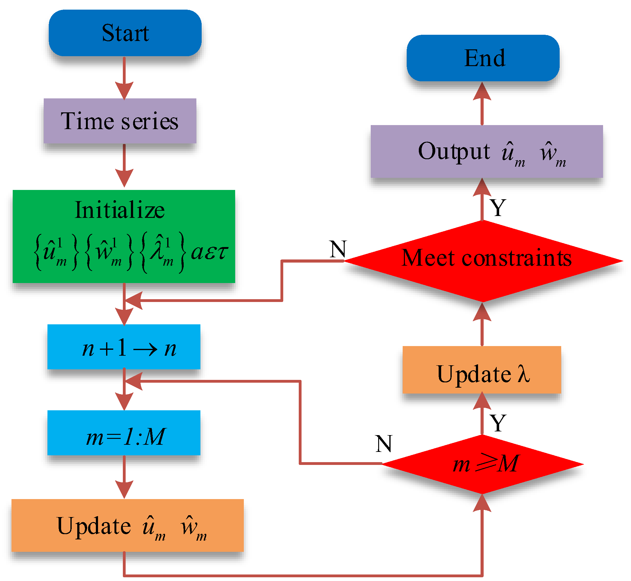
where $d$ denotes the offset parameter, $\epsilon$ denotes the convergence error line, and $\epsilon$ satisfies the condition of being greater than 0. The calculation flow of the variational mode decomposition is shown in Figure 1.

Figure 1 shows that the VMD decomposes the time series into a number of stable IMFs by removing noise and dividing the input signal in the frequency domain. Based on the finite bandwidth of each IMF, each IMF is predicted using its different centre frequencies, and the minimum value of the sum of the bandwidths is determined as the solution to the variational problem.

There are two gating units in the GRU, the update gate ($z$) and the reset gate ($r$), which are used to control the input of the function by adjusting the parameters, thus preserving the information of the useable value and eliminating useless and redundant data, which are good solutions for the problems of large fluctuations, slow convergence, and instability of the neural network caused by gradient disappearance and gradient explosion during operation. After the VMD decomposes the IMF, it is used as the input to the GRU, which is set at the time of $x_t$$t$, and the output of the hidden layer is $h_t$, which forms the candidate value ${\widehat{h}}_t$. The weights of the update gate are composed of $W_{zh}$ and $W_{zx}$; the weight matrix of the reset gate is composed of $W_{rh}$ and $W_{rx}$ ; the weight matrix of the hidden layer output candidate ${\widehat{h}}_t$ is $W_{hh}$ and $W_{hx}$; the output candidate value is obtained through these element operations (see Formula (6) for details).

$$\{\begin{array}{l}{z}_t=\sigma (W_{zh}{h}_{t-1}+W_{zx}{x}_t)\\ r_t=\sigma (W_{rh}{h}_{t-1}+W_{rx}{x}_t)\\ {\widehat{h}}_t=\tanh (W_{hh}(r_t\odot h_{t-1})+W_{hx}{x}_t)\\ h_t=(1-z_t)\odot h_{t-1}+{\widehat{h}}_t\odot z_t\end{array}$$

(6)

where $\sigma$ denotes the sigmoid function, $\sigma \in (0,1)$, which is responsible for activating the network; tanh denotes the hyperbolic tangent function, which belongs to (−1, 1); $\odot$ denotes the element product operation on the weight matrix. GRU uses the error between the input IMF value and the output value to adjust the weight parameters of the update gate, reset gate, and hidden layer, i.e., $W_z$, $W_r$, and $W_h$, respectively, in the process of continuous forward propagation to gradually obtain the optimal parameters, thus achieving the optimal prediction. By setting the input $y_t^i$ to $W_{v}h$ and the output $y_t^v$ to $\sigma (y_t^i)$, each weight parameter is calculated according to Formula (7).

$$\{\begin{array}{l}{W}_r=W_{rz}+W_{rh}\\ W_z=W_{zx}+W_{zh}\\ W_{\tilde{h}}=W_{\tilde{h}x}+W_{\tilde{h}h}\end{array}$$

(7)

The weight matrix is combined to form the parameter weights. The loss function of the moment $t$ is set to $E_t=0.5{(y_d-y_t^v)}^2$ and the loss function is used to converge the loss of the sample by performing a bias operation on each parameter weight. The update of each parameter after the convergence operation is shown in Formula (8).

$$\{\begin{array}{l}\frac{\partial E}{\partial W_{zx}}={\delta }_{z,t}{x}_t\\ \frac{\partial E}{\partial W_{zh}}={\delta }_{z,t}{h}_{t-1}\\ \frac{\partial E}{\partial W_{\widehat{h}x}}={\delta }_t{x}_t\end{array}$$

(8)

where $E$ denotes the loss of the sample. The GRU network reaches the optimum after training each parameter. The structure of the GRU gated recurrent unit is shown in Figure 2.

Figure 2 shows that the structure of the GRU consists of an update gate and a reset gate. In the update gate, the input at the moment determines the amount of information transferred between the upper and lower hidden layers through the sigmoid function, which reflects the GRU’s attention to historical data. In the gate, the activation function is used to determine the amount of information forgotten in the input at the moment, which reflects the update status of the information in the GRU network. Based on the gating unit and hidden layer, the analysis of information at each moment is realised, focusing on important information and ensuring the delivery of effective information. The short-term prediction process of the VMD-GRU algorithm is shown in Figure 3.

Figure 3 shows thatVMD-GRU prediction first requires the application of VMD to decompose the signal to reduce the complexity of the time series, and the resulting IMF is fed into the GRU network to make predictions after training parameters to achieve the monitoring of the health of civil and structural buildings.

3.2. WSN Civil Structural SHM Model Incorporating VMD-GRU

SHM can timely understand the health level of buildings by obtaining the durability and bearing capacity of current civil building structures. The incorporation of VMD-GRU in SHM provides risk prediction for the management of building structures, enabling problems to be identified and improved in a timely manner before hazards occur, which contributes to the sustainability of civil engineering buildings. Before VMD-GRU can make predictions, WSNs need to be used to distribute wireless sensor nodes in the monitoring area, enabling communication between the nodes so that information related to the health of the civil and structural building can be collected and processed. The sensor node coverage of the WSN is, thus, related to the comprehensiveness and accuracy of data collection and the efficiency of information transfer, which directly affects the assessment of the final building health level. Probabilistic sensing is used to understand the sensing range and sensing intensity of each node of the sensor, and this is used to adjust the node distribution to ensure comprehensive coverage. Assuming a target monitoring area of $S$, $K$ sensor nodes are randomly deployed within $S$. To ensure accuracy, the performance parameters of each node are set uniformly, and the coordinates of each node are $(x_n,y_n)$. Assuming that the node transmission range is a circle, with the sensor node’s own position as the centre, a circle for the effective sensing radius is drawn to obtain the coverage area of the sensor node $r$$c_n$; then, $c_n=(x_n,y_n,r)$. The coverage area of each sensor node is aggregated to form the set of sensor nodes $C=\left\{c_1,c_2,c_3,\dots ,c_N\right\}$. Assuming that the $S$ area consists of multiple equal pixels, each with an area of $a\times b$, the coordinates of each pixel point are $(x,y)$. The probability that each pixel point is within the coverage of the sensor node is $P\left\{r_n\right\}$, which can also be expressed as $P_{\mathrm{cov}}(x,y,c_n)$, where $r_n$ represents the pixel-point-covered event $P\left\{r_n\right\}$. See Formula (9) for the calculation.

$$P\left\{r_n\right\}=P_{\mathrm{cov}}(x,y,c_n)=\{\begin{array}{l}1, d(c_n,q)<r\\ 0, otherwise\end{array}$$

(9)

where $d(c_n,q)$ represents the distance between the node, $S$ is any point in the region, and its calculation is $Q(x_q,y_q)$, detailed in Formula (10).

$$d(c_n,q)=\sqrt{{(x_n-x_q)}^2+{(y_n-y_q)}^2}$$

(10)

The distance between the node $n$ and the node $q$ is the Euclidean distance, ${\lambda }_1$ and ${\lambda }_2$, obtaining the sensor node characteristics. Its calculation is shown in Formula (11).

$$\{\begin{array}{l}{\lambda }_1=r_e-r+d(c_n,p)\\ {\lambda }_2=r_e+r+d(c_n,p)\end{array}$$

(11)

where $r_e$ indicates the fluctuation range of sensor node monitoring, $r_e\in (0,r)$. Considering the actual monitoring environment of civil and structural buildings, it can be affected by the environment and interference from factors such as noise and high-frequency signals, which affect the accuracy of sensor node coverage. Probabilistic sensing is able to adjust the probability according to the changes in the environment and is highly adaptable, and the probability is calculated according to Formula (12).

$$P_{\mathrm{cov}}(x,y,c_n)=\{\begin{array}{l}1 d(c_n,q)\le r-r_e\\ e^{\frac{-{\alpha }_1{\lambda }_1{}^{{\beta }_1}}{{\lambda }_2{}^{{\beta }_2}+{\alpha }_2}\hspace{1em}\hspace{1em}\hspace{1em}\hspace{1em}\hspace{1em}\hspace{1em}\hspace{1em}\hspace{1em}\hspace{1em}}|d(c_n,q)-r|\le r_e\\ 0 d(c_n,q)\ge r+r_e\end{array}$$

(12)

The parameters ${\alpha }_1$, ${\alpha }_2$, ${\beta }_1$, and ${\beta }_2$ represent the probability of a node sensing a monitored target when the monitored target lies within the fluctuating range of the node’s monitoring. During the monitoring process, the sensing capability of the sensor node decreases with time and task, so it is often necessary to set a maximum value of target sensing probability $P_{\min }$ to limit the sensing behaviour of the node in order to improve the sensing accuracy of the node and maximise the role of the node. A monitored target is considered to be within range of a sensor node when its detection probability is greater than or equal to $P_{\min }$; otherwise, it means that the target is not sensed by the sensor node, i.e., the target is not included in the monitoring. To improve the quality of sensing, sensor nodes need to collaborate with each other to complete the sensing task in the monitoring area, so in the actual monitoring process, there will be multiple sensor nodes detecting the same target; probabilistic sensing needs to fuse the sensing probability of multiple nodes to determine the joint sensing probability, which is calculated according to Formula (13).

$$P_{\mathrm{cov}}(Cov)=1-{\displaystyle \prod _{n=1}^K(1-P_{\mathrm{cov}}(x,y,c_n))}$$

(13)

where $n$ is an integer in the range of [1, K]. The node coverage $P_{\mathrm{cov}}(x,y,c_{})$ determines whether the sensor nodes are within the coverage range, then the calculation of the coverage rate of the node set $R_{area}(C)$ refers to Formula (14).

$$R_{area}(C)=\frac{A_{area}(C)}{A_s}=\frac{{\displaystyle \sum _x^a{\displaystyle \sum _y^b{P}_{\mathrm{cov}}(x,y,c)}}}{a\times b}$$

(14)

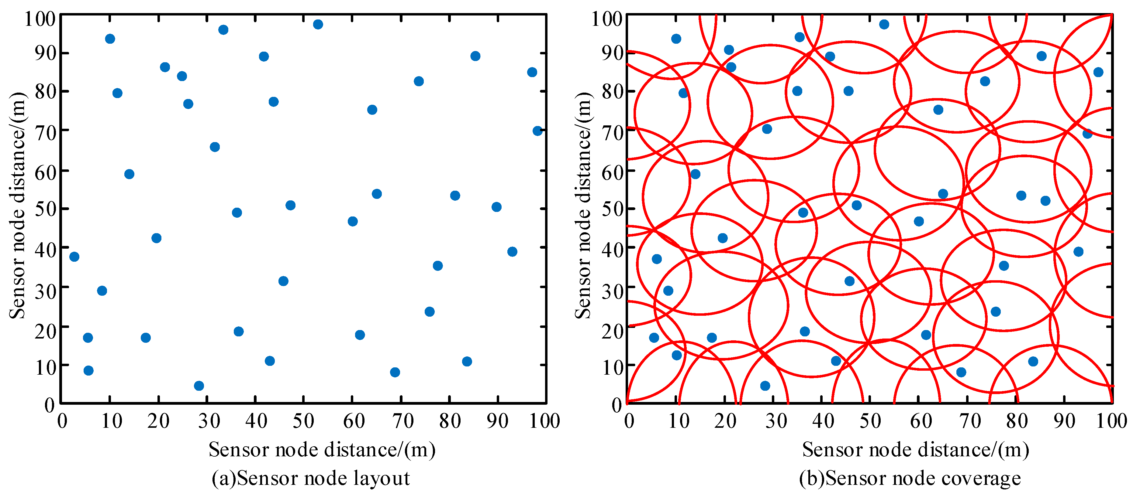
where $A_{area}(C)$ represents the coverage area of the node set $C$; $A_s$ represents the area of the monitoring area. The optimal scheme of node deployment is based on the selection of the best node. The best node needs to be determined by the ratio of the coverage area of the node set to the total area of the detection target area. The ratio is the largest, indicating that this node is the optimal node. The layout and coverage of wireless sensor nodes under probabilistic perception are shown in Figure 4.

Figure 4 shows thatunder probabilistic sensing, the distribution of wireless sensing nodes is more uniform, and their coverage is extensive, covering all areas without any loophole areas, so the wireless sensor network maintains a high coverage level in the monitoring area and achieves accurate positioning and real-time tracking of monitoring targets.

As the collected building structure data are numerous and complex, in order to improve the data quality and reduce the prediction error caused by the redundant data, it is necessary to normalise the data. On the premise of ensuring the integrity of the original information, abnormal and invalid data, including data with incorrect format, non-architectural structure data, and redundant data, are excluded. Dimensionality reduction operations are performed on all data information to reduce the amount of data as much as possible. Linear transformation is performed on the original data and mapped into the $a$ [0, 1] interval, and its calculation is detailed in Formula (15).

$$a^{\prime }=\frac{a-a_{\min }}{a_{\max }-a_{\min }}$$

(15)

where $a_{\max }$ denotes the maximum value of the linearly transformed data; $a_{\min }$ denotes the minimum value of the linearly transformed data. The structure of the WSN civil structural SHM model incorporating VMD-GRU is shown in Figure 5.

Figure 5 shows that the WSN civil structure SHM model incorporated into VMD-GRU consists of three layers: sensing layer, communication layer, and management layer. The WSN reasonably deploys sensor nodes to collect building structure data and form a building structure information database. High-quality information is obtained through data pre-processing and decomposed using VMD to obtain multiple IMFs before inputting them into the GRU model for prediction, and the obtained prediction results are used as a reference for assessing the assessment of the health level of the building structure.

4. Application of WSN Civil and SHM Models Incorporating VMD-GRU

4.1. Performance Analysis of the VMD-GRU Algorithm

The experiments were conducted with the Windows 10 operating system as the running condition and its hardware was an Intel Core i5-7300 CPU at 2.50 GHz with DDR48GB of memory. The signal was decomposed and the model was trained in a MATLAB 2020a environment. Two datasets, A and B, were selected to train and test the model. The A dataset and the B dataset contained 7548 and 7490 data samples, respectively. In both datasets, 80% were randomly selected as the training set, 10% as the test set, and 10% as the validation set. During the experiment, common intelligent algorithms for building structural health monitoring were added as experimental comparison, including the BP neural network (Back propagation neural network, BPNN) [27], GRU [28], and Support Vector Regression (SVR) [29]. The three algorithm models took the loss value and network consumption as the evaluation indicators of the model and evaluated the prediction error of the model and the network energy usage of the model. The parameter $K$ directly affects the accuracy and speed of VMD decomposition, so the optimal $K$ value needs to be determined experimentally to complete the construction of the VMD-GRU algorithm model. In the experiments of the A and B datasets, the comparison of the prediction errors of the VMD-GRU algorithm model under different $K$ values is shown in Figure 6.

Figure 6 shows that in the experiments on the two datasets, when $K$ was 6, the mean absolute error (MAE), root-mean-square error (RMSE), and mean absolute percent error (MAPE) were all the smallest, and the prediction accuracy was the highest. In Figure 6a, the MAE, RMSE, and MAPE for a value of 6 at $K$ were 0.03, 0.04, and 0.07 compared to 0.06, 0.04, and 0.08 for a value of 4 at $K$, respectively. In Figure 6b, the MAE, RMSE, and MAPE for a value of 6 at $K$ had the smallest values of 0.04, 0.05, and 0.07, respectively. MAE, RMSE, and MAPE reached the highest values of 0.07, 0.08, and 0.13, respectively. It can be seen that only when the parameter value was taken as 6, the gap between the predicted and real values was smallest and the prediction results closest to the real situation, which is conducive to giving full play to the advantages of VMD and laying the foundation for obtaining good prediction results.

The parameter $K$ for VMD in the VMD-GRU algorithm model was set to 6. The models were trained together with the comparison algorithm and the performance of each model was compared and analysed. The energy consumption of the network under different algorithm models in the A and B datasets is shown in Figure 7.

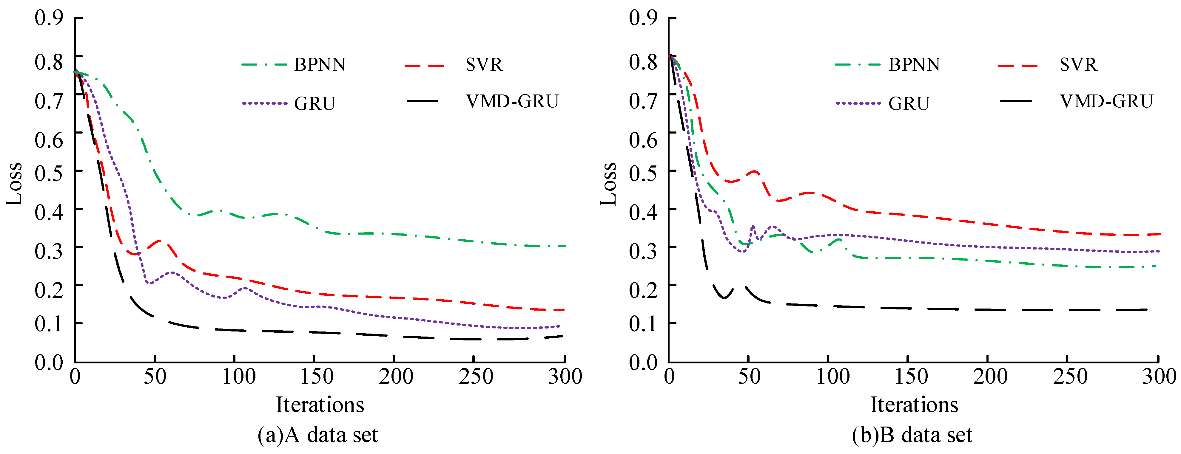
Figure 7 shows that the energy consumed by the VMD-GRU model network remained in the 0.05–1.0 Joule range during training in dataset A. The energy consumption was higher in the 20th, 80th, 130th, 200th, and 240th training rounds, exceeding 0.3 J overall, with high variability. The remaining energy consumption was all concentrated in the low-level range of 0–0.1 Joules. The GRU model had the largest fluctuation in energy consumption, with a minimum of less than 0.1 J and a maximum of up to 1.2 J, with a faster rate of energy change per round. The BPNN model and SVR model had higher levels of energy consumption, concentrated in the range of 0.6–1.0 Joules. In the training of dataset B, the energy consumed by the VMD-GRU model network was concentrated in the range of 0.1–0.5 Joules. The energy consumption of the remaining three models was concentrated in the range of 0.4–1.0 Joule sand fluctuated widely. It can be seen that the VMD-GRU model simplified the operational process, greatly reduced the network energy consumption, and was able to maintain a low and stable level of consumption. The comparison of the loss values of different algorithm models in the A and B datasets is shown in Figure 8.

Figure 8 shows that the loss value of the VMD-GRU model was lowest in both datasets of training. In dataset A, the VMD-GRU model maintained a stable loss value of 0.08 after 70 iterations, while in dataset B, the VMD-GRU model tended to have a loss value of 0.15 after 60 iterations. The BPNN was better trained in dataset B, with a stable loss value of 0.3 after 150 iterations. The loss value of GRU in dataset B improved by 0.2 compared to dataset A, and the number of iterations decreased by 70. This shows that the VMD-GRU model was able to achieve convergence at a faster rate and reach a low loss state, optimising the performance of the model.

4.2. Analysis of SHM Results for Civil Structures

A certain house building in a tourist attraction was used as a model application, and due to the training error, the study used 4 weeks to adjust the model parameters. Considering the influence of the sensor type and the number of sensor nodes on the model monitoring effect, the study selected three types, and 250, 260, and 270 sensors were selected for experiments at the same time. The prediction accuracy of the VMD-GRU model under different sensor types and number of sensor nodes is shown in Figure 9.

Figure 9 shows that under different sensor types, the prediction accuracy of the VMD-GRU model did not change much, the prediction accuracy of the three types of sensors basically remained in the range of 0.7, 0.85. The overall prediction accuracy of sensor type 1, sensor type 2 and sensor type 3 is about 0.8, 0.78 and 0.75 respectively, and the prediction accuracy difference between the three. If it did not exceed 0.1, the difference in prediction effect was not significant. At the same time, when the number of sensor nodes was 250, the prediction accuracy of the model was about 0.65. When the number of sensor nodes was 260 and 270, the prediction effect of the model was similar, and the accuracy was basically the same, about 0.85. Considering the equipment cost, we decided to use 260 sensor nodes to complete the monitoring of civil structures in an efficient and economical way.

A total of 260 sensors were used to monitor the building, of which 130 sensors were placed on the first and second floors; 13 sensors were placed on each civil structure truss; a 50 mm × 100 mm wire trough was used for the collection of wires and protection; shielded lines, water pipes, and load lines were laid under the truss monitoring points; the arrangement of sensor nodes was completed; the sample data collection time interval was set to 1.5 h; the collected building structure data were transmitted to the management through the base station and network. The management adopted an IoT-level structure, which consisted of the internet, wired and wireless communication networks, and cloud computing platforms to monitor the health of the civil and structural buildings, including the deformation and aging of materials, the degree of building corrosion, and the cracks and fractures of materials. A total of 8500 building structure data points were collected between June and September 2020 using showroom sensors, after data pre-processing as the final sample set. Three algorithmic models, BPNN [30], GRU [31] and SVR [32], were still used as experimental comparisons to analyse and test the monitoring performance of the models. The difference between the predicted value and the actual value under different algorithm models is shown in Figure 10.

Figure 10 shows that the overall predicted values of the VMD-GRU model for the health level of the building structure were closest to the real situation and had the highest prediction accuracy. The overall magnitude difference remained low at less than 0.01, except for the sample series of 70, where the magnitude difference reached a maximum level of 0.05. The SVR model produced a large magnitude difference in the prediction process, with the overall difference remaining in the range of 0.05–0.2. The SVR model produced magnitude values that differed significantly from the true values in the prediction of each sample series. The BPNN model had the lowest prediction accuracy, with predicted values differing significantly from the true values, both overall and for each sample series. The maximum difference in magnitude was 0.23, an improvement of 0.18 compared to the VMD-GRU model, and the smallest magnitude was 0.1, still at a high level. This shows that the VMD-GRU model was able to make full use of the advantages of VMD and GRU to achieve a high level of accuracy in predicting the health levels of civil and structural buildings. The comparison of MAE, RMSE, and MAPE values under different algorithm models is shown in Figure 11.

Figure 11 shows that the MAE, RMSE, and MAPE values of the VMD-GRU model were significantly different from the other models. In Figure 10a, the GRU model had the highest MAE value of approximately 0.08; the VMD-GRU model had the smallest MAE value of approximately 0.03, which was 0.02 and 0.04 lower compared to the BPNN and SVR models, respectively. In Figure 10b, the RMSE value was the lowest among the VMD-GRU models at 0.04, followed by the BPNN model with an RMSE value of approximately 0.05, and the SVR model had the highest RMSE value of over 0.08. In Figure 10c, the VMD-GRU model achieved the lowest MAPE value of 0.06, which was 0.05, 0.07, and 0.06 lower than the BPNN, GRU, and SVR models, respectively, and overall, the VMD-GRU model had the smallest average magnitude of error, which indicates that its predicted value was closest to the true value. Thus, the VMD-GRU model optimises the prediction effect and improves the model performance, which can improve a reliable reference for civil construction assessment.

5. Conclusions

SHM is the basis for improving the durability and safety of building structures, which is conducive to maintaining building structures and reducing engineering accidents. In order to optimise the effect of SHM in civil and structural buildings, the study proposed the improvementof the WSN-based SHM model using the VMD-GRU algorithm, and the accuracy of the constructed index system model was verified. In the training process of the model, the improved model achieved the minimum value levels of 0.03, 0.04, and 0.07 for MAE, RMSE, and MAPE, respectively, when the value of VMD parameter $K$ was 6, with the smallest error and the best prediction results. In the decomposition method of VMD, the $K$ value determines the number of IMFs and has an important influence on the decomposition effect. If the $K$ value is too small, it is easy to cause insufficient decomposition, inherent modal confusion, and overlap, which increases the complexity of the data; $K$ data redundancy reduces data availability. It can be seen that whether the $K$ value is too large or too small, it reduces the quality of the original data to a certain extent, adversely affects the subsequent prediction, and causes prediction errors. Therefore, choosing an appropriate $K$ value is the guarantee to improve the prediction effect of the VMD-GRU model.

In the training in dataset A, the energy consumed by the VMD-GRU model network remained in the range of 0.05–1.0; in the training in dataset B, the energy consumed by the VMD-GRU model network was concentrated in the range of 0.1–0.5. The energy consumption was reduced by 0.05–0.2 and 0.1–0.5 for datasets A and B, respectively, compared to the GRU model. The number of iterations was stable around 60 and the loss value remained stable at 0.1. It can be seen that the VMD-GRU model had a faster convergence speed and higher network resource utilisation. VMD uses iterative search to find the optimal solution of modal decomposition, which reduces the complexity of the original data, improves the convenience of data utilisation, and realises the effective decomposition of time series. GRU simplifies the gate mechanism structure, reduces the parameters that need to be used by removing the output gate, improves the scalability of the GRU network, and reduces the risk of overfitting. At the same time, GRU converts the continuous multiplication operation of the activation function derivative into an addition operation, which reduces the complexity and difficulty of the calculation, which is conducive to speeding up the convergence speed of the model, reducing the number of iterations, and improving the operating efficiency of the model.

In the practical application of the model, the overall predicted values of the VMD-GRU model building structure health level were closest to the real situation and had the highest prediction accuracy. The MAE, RMSE, and MAPE were 0.03, 0.04, and 0.06, which were 0.06, 0.02, and 0.07 lower than those of the GRU model, respectively. The VMD-GRU model used VMD decomposition to reduce data errors caused by factors such as noise and outliers, improved the standardisation and availability of building structure data, and provided a good foundation for VMD-GRU model prediction; the VMD-GRU model usedthe GRU method for prediction of civil structure buildings, feature filtering was realised through the update gate and reset gate of GRU, invalid data were eliminated, and important and valuable information was retained. This research helps to understand the global search ability of the optimal solution, further enhances the prediction ability of the model, and provides technical support for the structural health monitoring of buildings.

To sum up, the VMD-GRU model improves the efficiency of health monitoring of civil structure buildings, reduces the prediction error, optimises the monitoring effect, is beneficial to the management and utilisation of civil structure buildings, and improves its social and economic value. Although the research has achieved certain results, there is still the limitation of a small sample data size. In future research, it is necessary to expand the sample size to further verify the results of this research.

References

- Nichols, J.M.; Tomor, A.K.; Benedetti, A. Development of a time-dependent structural reliability model for civil engineering structures. Mason. Int. 2019, 32, 72–79. [Google Scholar]
- Xiao, X.; Mu, B.; Cao, G.; Yang, Y.; Wang, M. Flexible battery-free wireless electronic system for food monitoring. J. Sci. Adv. Mater. Devices 2022, 7, 100430. [Google Scholar] [CrossRef]
- Wu, H.; Jin, S.; Yue, W. Pricing policy for a dynamic spectrum allocation scheme with batch requests and impatient packets in cognitive radio networks. J. Syst. Sci. Syst. Eng. 2022, 31, 133–149. [Google Scholar] [CrossRef]
- Zheng, H.; Jin, S. A multi–source fluid queue based stochastic model of the probabilistic offloading strategy in a MEC system with multiple mobile devices and a single MEC server. Int. J. Appl. Math. Comput. Sci. 2022, 32, 125–138. [Google Scholar]
- Zonzini, F.; Aguzzi, C.; Gigli, L.; Sciullo, L.; Testoni, N.; De Marchi, L.; Di Felice, M.; Cinotti, T.S.; Mennuti, C.; Marzani, A. Structural health monitoring and prognostic of industrial plants and civil structures: A sensor to cloud architecture. IEEE Instrum. Meas. Mag. 2020, 23, 21–27. [Google Scholar] [CrossRef]
- Sui, T.; Marelli, D.; Sun, X.; Fu, M. Multi-sensor state estimation over Lossy channels using coded measurements. Automatica 2020, 111, 108561. [Google Scholar] [CrossRef]
- Wang, Y.; Han, X.; Jin, S. MAP based modeling method and performance study of a task offloading scheme with time-correlated traffic and VM repair in MEC systems. Wirel. Netw. 2022. [Google Scholar] [CrossRef]
- Sun, W.; Lv, X.; Qiu, M. Distributed estimation for stochastic Hamiltonian systems with fading wireless channels. IEEE Trans. Cybern. 2022, 52, 4897–4906. [Google Scholar] [CrossRef]
- Pal, P.; Sharma, R.P.; Tripathi, S.; Kumar, C.; Ramesh, D. 2.4 GHz RF received signal strength based node separation in WSN monitoring infrastructure for millet and rice vegetation. IEEE Sens. J. 2021, 21, 18298–18306. [Google Scholar] [CrossRef]
- Liu, Z.; He, Q.; Li, Z.; Peng, Z.; Zhang, W. Vision-based moving mass detection by time-varying structure vibration monitoring. IEEE Sens. J. 2020, 20, 11566–11577. [Google Scholar] [CrossRef]
- Zhou, X.; Bai, Y.; Nardi, D.C.; Wang, Y.; Wang, Y.; Liu, Z.; Picón, R.A.; Flórez-López, J. Damage evolution modeling for steel structures subjected to combined high cycle fatigue and high-intensity dynamic loadings. Int. J. Struct. Stab. Dyn. 2022, 22, 2240012. [Google Scholar] [CrossRef]
- Zhang, C.; Mousavi, A.A.; Masri, S.F.; Gholipour, G.; Yan, K.; Li, X. Vibration feature extraction using signal processing techniques for structural health monitoring: A review. Mech. Syst. Signal Processing 2022, 177, 109175. [Google Scholar] [CrossRef]
- Xi, Y.; Jiang, W.; Wei, K.; Hong, T.; Cheng, T.; Gong, S. Wideband RCS reduction of Microstrip antenna array using coding Metasurface with low Q resonators and fast optimization method. IEEE Antennas Wirel. Propag. Lett. 2022, 21, 656–660. [Google Scholar] [CrossRef]
- Wang, Z.; Cha, Y.J. Unsupervised deep learning approach using a deep auto-encoder with an one-class support vector machine to detect structural damage. Struct. Health Monit. 2020, 20, 406–425. [Google Scholar] [CrossRef]
- Guo, L.; Li, R.; Jiang, B. A cascade broad neural network for concrete structural crack damage automated classification. IEEE Trans. Ind. Inform. 2020, 17, 2737–2742. [Google Scholar] [CrossRef]
- Wang, C.; Xiao, J.; Zhang, C.; Xiao, X. Structural health monitoring and performance analysis of a 12-story recycled aggregate concrete structure. Eng. Struct. 2020, 205, 110102. [Google Scholar] [CrossRef]
- Carratu, M.; Espirito-Santo, A.; Monte, G.; Paciello, V. Earthquake early detection as an IEEE1451 transducer network trigger for urban infrastructure monitoring and protection. IEEE Instrum. Meas. Mag. 2020, 23, 43–49. [Google Scholar] [CrossRef]
- Zhang, H.; Yu, L.; Ma, S.; Cao, S.; Xia, Q.; Liu, Y.; Zhang, H. Adaptive sparse reconstruction of damage localization via Lamb waves for structure health monitoring. Computing 2019, 101, 679–692. [Google Scholar] [CrossRef]
- Wu, Y.; Liu, X.; Chen, B.; Li, Q.; Luo, P.; Pronk, A. Design, construction and monitoring of an ice composite shell structure. Autom. Constr. 2019, 106, 102862. [Google Scholar] [CrossRef]
- Peckens, C.; Cook, I.; Fogg, C. Bio-inspired sensing and actuating architectures for feedback control of civil structures. Bioinspiration Biomim. 2019, 14, 1748–3190. [Google Scholar] [CrossRef]
- Shen, W.; Niyitangamahoro, A.; Feng, Z.; Zhu, H. Tuned inerter dampers for civil structures subjected to earthquake ground motions: Optimum design and seismic performance. Eng. Struct. 2019, 198, 109470. [Google Scholar] [CrossRef]
- Li, Z.; Fu, J.; Liang, Q.; Mao, H.; He, Y. Modal identification of civil structures via covariance-driven stochastic subspace method. Math. Biosci. Eng. 2019, 16, 5709–5728. [Google Scholar] [CrossRef] [PubMed]
- Raffaele, L.; Bruno, L. Windblown sand action on civil structures: Definition and probabilistic modelling. Eng. Struct. 2019, 178, 88–101. [Google Scholar] [CrossRef]
- De-La-Colina, J.; Arias-Lara, D.; Valdés-González, J. Effect of noise on the assessment of displacements computed from accelerations recorded at linear and nonlinear civil engineering structures. Measurement 2019, 136, 724–734. [Google Scholar] [CrossRef]
- Li, Y.; Bao, T.; Gao, Z.; Shu, X.; Zhang, K.; Xie, L.; Zhang, Z. A new dam structural response estimation paradigm powered by deep learning and transfer learning techniques. Struct. Health Monit. 2021, 21, 770–787. [Google Scholar] [CrossRef]
- Tibaduiza, D. Temperature prediction using multivariate time series deep learning in the lining of an electric arc furnace for ferronickel production. Sensors 2021, 21, 6894. [Google Scholar]
- Zhang, P.; Cui, Z.; Wang, Y.; Ding, S. Application of BPNN optimized by chaotic adaptive gravity search and particle swarm optimization algorithms for fault diagnosis of electrical machine drive system. Electr. Eng. 2021, 104, 819–831. [Google Scholar] [CrossRef]
- Shu, W.; Cai, K.; Xiong, N.N. A short-term traffic flow prediction model based on an improved gate recurrent unit neural network. IEEE Trans. Intell. Transp. Syst. 2021, 23, 16654–16665. [Google Scholar] [CrossRef]
- Leibold, C. Neural kernels for recursive support vector regression as a model for episodic memory. Biol. Cybern. 2022, 116, 377–386. [Google Scholar] [CrossRef]
- Gao, D.; Hu, B.; Qin, F.; Chang, L.; Lyu, X. A real time gravity compensation method for INS based on BPNN. IEEE Sens. J. 2021, 21, 13584–13593. [Google Scholar] [CrossRef]
- Fu, B.; Yuan, W.; Cui, X.; Yu, T.; Zhao, X.; Li, C. Correlation analysis and augmentation of samples for a bidirectional gate recurrent unit network for the remaining useful life prediction of bearings. IEEE Sens. J. 2021, 21, 7989–8001. [Google Scholar] [CrossRef]
- Jassim, M.S.; Coskuner, G.; Zontul, M. Comparative performance analysis of support vector regression and artificial neural network for prediction of municipal solid waste generation. Waste Manag. Res. 2022, 40, 195–204. [Google Scholar] [CrossRef] [PubMed]
Figure 1.
The calculation flow of the variational mode decomposition.
Figure 2.
GRU gate control cycle unit structure.
Figure 3.
Short-term prediction process of VMD-GRU algorithm.
Figure 4.
Placement and coverage of wireless sensor nodes based on probability perception.
Figure 5.
WSN civil structure SHM prediction model structure integrated with VMD-GRU.
Figure 6.
Comparison of prediction errors of VMD-GRU algorithm models under different K values.
Figure 7.
Comparison of network energy consumption under different algorithm models in A and B datasets.
Figure 8.
Comparison of loss values of different algorithm models in A and B datasets.
Figure 9.
Prediction accuracy of VMD-GRU model under different sensor types and number of sensor nodes.
Figure 10.
Comparison of the difference between the predicted value and the real value under different algorithm models.
Figure 11.
Comparison of MAE, RMSE, and MAPE values under different algorithm models.
Publisher’s Note: MDPI stays neutral with regard to jurisdictional claims in published maps and institutional affiliations. |
© 2022 by the author. Licensee MDPI, Basel, Switzerland. This article is an open access article distributed under the terms and conditions of the Creative Commons Attribution (CC BY) license (https://creativecommons.org/licenses/by/4.0/).
Share and Cite
MDPI and ACS Style
Liu, Y. WSN-Based SHM Optimisation Algorithm for Civil Engineering Structures. Processes 2022, 10, 2113. https://doi.org/10.3390/pr10102113
AMA Style
Liu Y. WSN-Based SHM Optimisation Algorithm for Civil Engineering Structures. Processes. 2022; 10(10):2113. https://doi.org/10.3390/pr10102113
Chicago/Turabian StyleLiu, Ying. 2022. "WSN-Based SHM Optimisation Algorithm for Civil Engineering Structures" Processes 10, no. 10: 2113. https://doi.org/10.3390/pr10102113
Note that from the first issue of 2016, this journal uses article numbers instead of page numbers. See further details here.