A Practical Field Test and Simulation Procedure for Prediction of Scaling in Geothermal Wells Containing Noncondensable Gases

Abstract

Scaling in a hydrothermal type of geothermal well reduces or interrupts the production of geothermal energy. Calcite is one of the most common scales in geothermal wells. The reason for its formation in geothermal production wells is clear. The flowing up of geothermal water causes a change in the pressure and temperature, which results in the escape of CO₂ gas from the geothermal water, causing a rise in pH and the supersaturation of CaCO₃ in the solution. To predict scaling in a new geothermal well, conditional data for geothermal well simulations are required. It is important to determine what field data are needed and how to obtain them. It is necessary to deal with some parameters that are hard to measure and that have not been described in detail in the existing literature. In this study, a two-phase flow model and a chemical reaction equilibrium model are integrated to simulate the scaling process in production wells. Based on the simulation, a comprehensive and practical approach, including a novel noncondensable gas content measurement method, is applied to predict the depth of the first gas bubble using simple field test data and does not require reservoir permeability and earth conductivity. The result shows good agreement with the location of scaling detected in the field.

1. Introduction

At present, the main global energy consumption still relies on fossil fuels, which brings problems, such as environmental pollution and climate change. Thus, it is urgent for us to change our energy use to new or renewable energy resources. Geothermal energy is an important renewable energy. It has the characteristics of large reserves, wide distribution and is clean, stable and reliable. It originates from the Earth’s magma and the decay of radioactive materials. Geothermal energy is usually divided into shallow, hydrothermal and hot dry rock categories. In the process of geothermal energy extraction from either hydrothermal geothermal reservoirs or hot dry rock by enhanced geothermal systems [1], due to changes in fluid temperature and pressure and the occurrence of chemical reactions, scaling may occur in geothermal wells and surface equipment [2,3], which will block fluid flowing in pipelines and result in loss or even cessation of production.

Scholars around the world have carried out a large number of studies on this topic. Yanagisawa et al. [1] studied scaling in a hot dry rock geothermal system in Hijiori, Japan. They found that after long-term operation, scales appeared in several different locations due to changes in temperature. Mohammad Zolfagharroshan et al. [4] established a calculation model for geothermal well flow and scaling, which is highly consistent with the actual test data. Zhang et al. [5] tested the performance of a calcium carbonate-scale crystal growth kinetics model through an experiment on scaling in geothermal water blocking flow in pipes and applied it to predict carbonate scaling in a North Sea well. The results showed that the prediction was in good agreement with the real experimental field test results. Tut Haklıdır et al. [6] provided a review of mineral precipitation and effective scale inhibition methods at geothermal power plants in West Anatolia (Turkey). They pointed out that the systematic physical and chemical monitoring studies are critical for providing uninterrupted energy production from power plants. They discussed the selection of suitable chemical inhibitors, identifying optimum dosages of inhibitors along with correct dosage points, and showed that preparing correct dilutions with water for each geothermal system can extend the lifetime of geothermal power plant wells and equipment. Zhang et al. [7] used geothermal water from Xining Basin, China, to conduct scaling reaction tests under different temperatures, pressures and partial pressures of CO₂ and found that only a very small amount of scale particles can attach to the pipe wall, while most of them will invade the formation and damage the injectivity.

An exponential model is an important basis for judging the scaling trend. Song et al. [8] predicted the scaling and corrosion tendencies of geothermal water by using Langelier and Larson index (two kinds of CaCO₃ saturation prediction indexes) models and verified it by a static immersion test. The results show that Langelier index can better predict the scaling tendency of the aerated geothermal water, especially for the geothermal water with a serious scaling potential. Wang et al. [9] analyzed the water quality of a geothermal well in Ganzi, Sichuan province, China, and judged the tendency of corrosion and scaling according to a Larson index and a Ryzner index. The results showed that the geothermal water in this area had a moderate tendency to cause scaling and the scale component was CaCO₃. Liu [10] pointed out that there is still relatively little work on the prediction of the corrosion and scaling tendency of geothermal fluids and suggested systematic analysis of the corrosion and scaling tendency, three-dimensional multiphase flow and chemical reaction numerical simulation based on the characteristics of geothermal fluids in different regions are the future directions for research. Zhu et al. [11] discussed the method for judging the scaling and corrosion tendency of geothermal water. When the Cl⁻ content of geothermal water is greater than 25%, the Larson index is better than the Ryzner index for judging the tendency for scaling.

Prevention or removal of scale in geothermal systems usually requires the use of scale inhibitors and appropriate manipulation of injection to achieve good results. Haklidir et al. [12] designed two fuzzy logic controllers to control silica and calcium carbonate scale inhibition systems and achieved good results. Topcu et al. [13] investigated the effect of CO₂ injection on the formation of scaling in Tuzla Geothermal Field (TGF), located in the northwest of Turkey. The results show that the injection of CO₂ into the hypersaline brine of TGF is a promising green approach for both mitigation of scaling by reducing pH at the well head and the minimization of potential corrosion compared to the use of formic acid. Zhang et al. [14] used PHREEQC, a software developed by The US Geological Survey, to analyze and study the scaling problem of a high-temperature geothermal well in Kangding, China, by using hydrogeochemical simulation technology. The results show that serious scale formation occurs with the change in temperature, pH, pressure and redox environment of the geothermal fluid during exploitation.

To solve the scaling problem, chemical scale inhibitors or mechanical removal are needed in geothermal wells. However, chemical scale inhibitors need to be added to pure liquid geothermal water to achieve good scale inhibition [15,16], so it is very important to determine the depth of the first gas bubble in geothermal wells. The point where the wellbore dynamic pressure profile diverges from linearity is generally used for determining gas breakout depth. However, a significant amount of vaporization must have occurred to change the slope of the line and lead to curvature in the pressure profile. Moreover, the depth of that point is most probably shallower than the depth of the first gas bubble. The pH changes as soon as a gas bubble forms [16]. Therefore, it is not sensitive to use dynamic pressure curve to predict the depth of the first gas bubble and a more accurate calculation model is needed. Pátzay et al. [17] developed an equilibrium simulation algorithm and a computer program for calcite scale formation in a CaCO₃–H₂O-CO₂ system using the Davies and Pitzer activity calculation methods and a simple linearization method to deal with the flow pressure drop and temperature change in the well. Haizlip et al. [15] discussed the influence of noncondensable gases on reservoir and geothermal well productivity. In their study, the partial pressure of CO₂ dissolved in geothermal water was calculated using Henry’s law and the steam tables. The depth of gas breakout (bubble) depth in high gas content wells can be estimated using the measured downhole pressures from dynamic surveys and the calculated total pressure where the total pressure is the sum of the liquid water pressure plus the gas pressure. Akin [16] et al. used the geothermal water composition, CO₂ gas content and wellbore temperature and pressure data to calculate the bubble starting point position in PHREEQC software. Pátzay et al. [18] used a solubility equilibrium program GEOPROF to determine the bubble point depth, temperature and pressure, as well as the partial pressure profiles of the gases CO₂, CH₄ and N₂ in two geothermal wells in southern Hungary. It was recommended that the wellhead pressure should be maintained above 40 bar in one of the wells because of the intensity of scaling at surface conditions. Liang et al. [19] used WellSim, a well simulation software, to predict the location of scaling in a geothermal well in Hebei province, China, and analyzed the impact of scaling. When preventing scaling on site, the depth of the submersible pump or the injection of scaling inhibitor should be below the flash point.

As far as we know, most of the literature on scaling simulations in geothermal wells used existing commercial software (such as WellSim, PHREEQC) or only introduced briefly the simulation calculation. However, geothermal fluid scaling involves two-phase flow and chemical reaction. For example, the model of reference [4] mainly focused on two-phase flow cannot simulate the change in chemical components and analyze the effect of noncondensable gases on scaling. The model in reference [17] focused on chemical equilibrium but without concerning detailed two-phase flow fluid dynamics. In addition, to predict scaling in a new geothermal well, conditional data for geothermal well simulations are required. What field data are needed and how to obtain them has not been described in detail in the previous literature. In this paper, the whole process of specific simulation methods and field data acquisition methods are integrated and clarified. In this study, we will take a geothermal well in Boye, Hebei province, China, as an example to systematically elaborate the methodology.

2. Wellbore Simulation

2.1. Mathematical Model

The basic mechanism of wellbore scaling is as follows: while the geothermal fluid rises from underground through a wellbore, the pressure decreases continuously and flashing may appear somewhere in the wellbore. Then, acidic gaseous CO₂ originally dissolved in geothermal water solution escapes into the steam, which raises the solution pH and results in super-saturation of CaCO₃ solubility and, therefore, precipitation of solid scale.

Although the principle of CaCO₃ scaling in a wellbore has been recognized, accurate modeling of it is quite complicated, involving two-phase flow, formation heat transfer and chemical changes in the solution and especially the flash process. Thus, the model should involve chemical reaction equilibrium and phase equilibrium of the brine in the wellbore, pressure drop in the two-phase flow and heat loss to the formation, etc. The mathematical model of these processes presented in this paper is based on references [4,20,21,22].

2.1.1. Two-Phase Flow Model

The conservation equations for the fluid are given below in one-dimensional form:

Continuity:

$$\frac{\partial \rho }{\partial t}+\frac{\partial \left(\rho v\right)}{\partial l}=0$$

(1)

where ρ is the fluid density in kg/m³, v is the velocity in m/s; t is time in s and l is the wellbore length in m. There is no mass accumulation in steady-state flow. Therefore, we have:

$$\frac{\partial \left(\rho v\right)}{\partial l}=0$$

(2)

Momentum:

$$\frac{\partial \left(\rho v\right)}{\partial t}+\frac{\partial \left(\rho v^2\right)}{\partial l}=-\frac{\partial p}{\partial l}-\tau \frac{\mathsf{\pi }d}{A}-\rho g\sin \theta$$

(3)

where p is pressure in Pa, τ is the frictional coefficient in kg/(m∙s²), d is the wellbore inner diameter in m, A is the wellbore cross sectional area in m², g is the gravitational acceleration in m/s² and θ is the angle between the wellbore and the horizontal direction (dimensionless). Considering steady-state flow and by combining Equations (2) and (3), Equation (3) can be reduced to

$$\frac{\mathrm{d}p}{\mathrm{d}l}=-\tau \frac{\mathsf{\pi }d}{A}-\rho g\sin \theta -\rho v\frac{\mathrm{d}v}{\mathrm{d}l}$$

(4)

When it flashes to two-phase flow, the fluid is regarded as a homogeneous gas–liquid mixture. If the well is vertical, Equation (4) can be written as follows:

$$-\frac{\mathrm{d}p}{\mathrm{d}z}=g{\rho }_{\mathrm{mix}}+\frac{f_{\mathrm{mix}}{v}_{\mathrm{mix}}^2{\rho }_{\mathrm{mix}}}{2d}+{\rho }_{\mathrm{mix}}{v}_{\mathrm{mix}}\frac{\mathrm{d}{v}_{\mathrm{mix}}}{\mathrm{d}z}$$

(5)

where z is the vertical length in m, f is the friction factor (dimensionless) and the subscript mix stands for mixture parameters. In our study, the friction factor calculation model from reference [20] is adopted. Here, we will not repeat related equations from the reference. The void fraction and mixing density are used to calculate different friction factors according to different flow patterns. Flow patterns of gas–liquid two-phase flow can be classified into four types: Bubbly, Slug, Churn and Annular. Slip effects are considered in all these flow regimes.

Energy:

$$\frac{\mathrm{d}h}{\mathrm{d}l}=-v\frac{\mathrm{d}v}{\mathrm{d}l}-g\sin \theta -\frac{\mathrm{d}q}{\mathrm{d}l}$$

(6)

where h is enthalpy in J/kg and q is the heat transfer rate per unit of mass flow rate of a calculation section in W/(kg/s), defined by [21] as:

$$q=\frac{l\mathsf{\pi }dU\left(T-T_{\mathrm{ei}}\right)}{m_{\mathrm{f}}}$$

(7)

where l is the length of a calculated wellbore section in m, m_f is mass flow rate in kg/s, T_ei is the formation temperature in K and U is the total heat transfer coefficient in W/(m²∙K). U may be approximated by [23]

$$U=\frac{0.6k}{d}$$

(8)

where k is the “effective thermal conductivity” of the formation [24]. For steady-state liquid flow through a wellbore, k can be estimated by matching the temperature profile in the well [21].

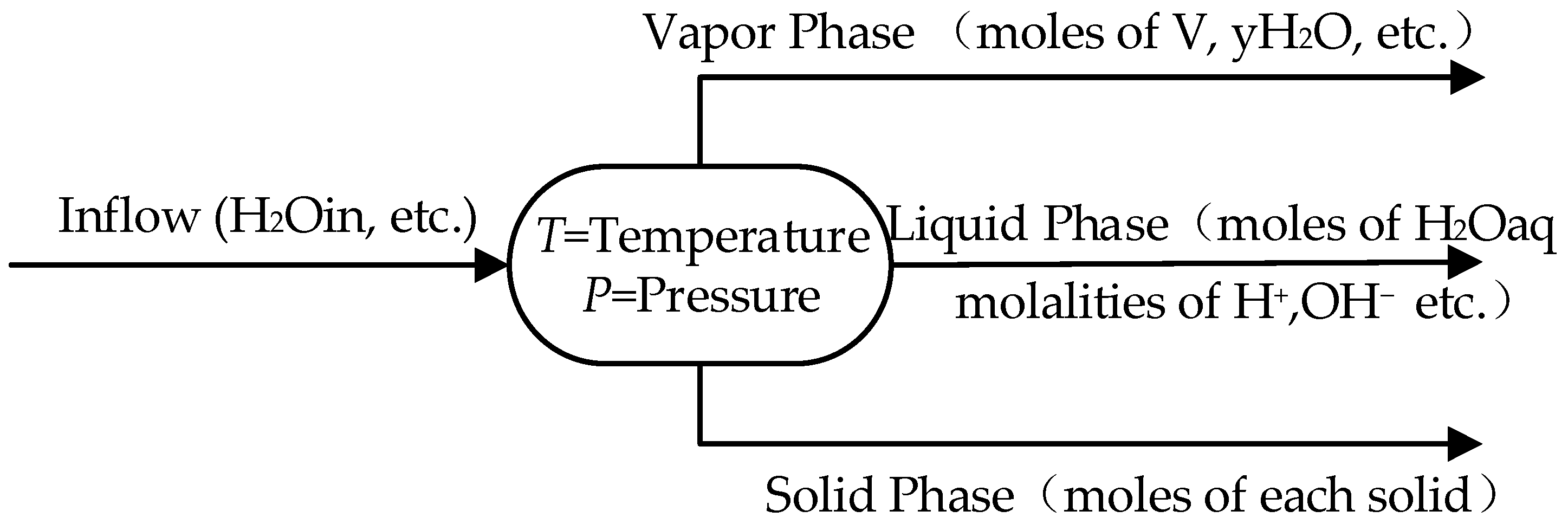
2.1.2. Chemical and Phase Equilibrium Models

The electrolyte solution phase equilibrium model [22] is used as a reference to calculate the flash process. The phase equilibrium model of an electrolyte solution is shown in Figure 1. After the change in temperature and pressure of the incoming solution, containing certain amounts of chemical components, its chemical components are redistributed among the three phases of gas, liquid and solid.

The equations involved are as follows.

Mass equilibrium of chemical components can be expressed as

$$F_{\mathrm{out},i}=F_{\mathrm{in},i}+\sum _{j=1}^M{v}_{i,j}{\xi }_j$$

(9)

where F_in,i and F_out,i are the molar flow rates of each component i before and after ionization or dissociation reaction, respectively, in mol/s, ν is the stoichiometric coefficient (dimensionless), ξ is the reaction degree in mol/s, j stands for a certain equilibrium equation and M is the total number of equilibrium equations.

Therefore, the updated chemical component compositions after chemical reactions have reached equilibrium can be defined by

$$z_i=\frac{F_{\mathrm{out},i}}{{\sum }_i^N{F}_{\mathrm{out},i}}$$

(10)

where N is the total number of chemical components. The total mass equilibrium can be described by the following equations.

$$\begin{array}{l}F=L+V\\ F{z}_i=L{x}_i+V{y}_i\end{array}$$

(11)

where F is the total mass flow rate of all phases in mol/s, L liquid phase, V gas phase, x is the liquid phase ratio, y is the gas phase ratio and z is the chemical component compositions in all phases.

The energy balance is shown in the following equation.

$$H_{\mathrm{L}}L+H_{\mathrm{V}}V=H_{\mathrm{F}}F+Q$$

(12)

where H_L, H_V and H_F are the molar enthalpy of liquid, gas and all phases in J/mol; Q is the heat transfer rate in W.

Phase equilibrium is shown in the following equation.

$$y_i=K_i{x}_i$$

(13)

where K is the Henry coefficient (dimensionless). According to Henry’s law, the solubility of a gas in a liquid (expressed by mole fraction) is proportional to the equilibrium partial pressure of the gas at a certain temperature and equilibrium state.

Chemical equilibrium can be expressed by the following equation.

$$K_j=\prod _{i=1}^N{\left({\gamma }_i{x}_i\right)}^{{\nu }_{ij}}=\prod _{i=1}^N{\left(\frac{p_i{\widehat{\varphi }}_i}{f_i^0}\right)}^{{\nu }_{ij}}$$

(14)

where K is the chemical reaction equilibrium constant, where the dimension is different for each specific chemical reaction, γ is the activity coefficient in dimensionless, φ is the fugacity coefficient in dimensionless and f is the fugacity in Pa. Pitzer electrolyte activity coefficient model [25] was used to calculate the liquid phase activity coefficients, while gas phase fugacity coefficients were calculated by a PR equation of state [26].

The chemical constituent constraint can be expressed by the following equations.

$$\begin{gathered} \sum _{i=1}^{N_{\mathrm{m}}}{y}_i=1 \\ \sum _{i=1}^N{x}_i=1 \end{gathered}$$

(15)

where N_m is the total number of gas molecules and m stands for molecular.

The electroneutral equilibrium can be shown as the following equations.

$$\sum _{i=1}^N{Z}_i{x}_i=0$$

(16)

Here, Z_i represents the true value of the charge of the ion species, not the absolute value, without dimension.

Physical property correlations are shown by the following equations.

$$\begin{array}{l}{H}_{\mathrm{F}}=H\left(P_{\mathrm{F}},T_{\mathrm{F}},z_i\right)\\ H_{\mathrm{V}}=H\left(P,T,y_i\right)\\ H_{\mathrm{L}}=H\left(P,T,x_i\right)\\ K_i=K\left(P,T,x_i,y_i\right)\\ K_j=K\left(T,P\right)\end{array}$$

(17)

2.1.3. Scaling Tendency

A saturation index model is used in this paper to predict the scaling tendency of geothermal fluid. The saturation index is defined by

$$\mathrm{SI}=\lg \frac{\left\{\left[\mathrm{Me}\right]\left[\mathrm{An}\right]\right\}}{K_{\mathrm{sp}}}$$

(18)

where [Me] and [An] are bivalent cation and anion concentrations, respectively, and K_sp is solubility. When the SI is equal to zero, [Me][An] is saturated in the solution; when SI is larger than zero, [Me][An] is super-saturated and there is a tendency for scaling.

For calcite, the following equation for the SI correlation is adopted [4].

$$\begin{array}{l}\mathrm{SI}=\lg \left[\frac{\left[{\mathrm{Ca}}^{2+}\right]\left[{\mathrm{HCO}}_3^{2-}\right]}{P{y}_{\mathrm{g}}^{{\mathrm{CO}}_2}{f}_{\mathrm{g}}^{{\mathrm{CO}}_2}}\right]+6.33+15.0\times {10}^{-3}T-\\ 5.31\times {10}^{-6}{T}^2-5.27\times {10}^{-5}P-3.334S_i^{0.5}+1.431S_i\end{array}$$

(19)

where T is the temperature in °C, P is the pressure in psi and S is the ion strength, defined by

$$S=\frac{1}{2}{\displaystyle \sum _{i=1}^N{C}_i{Z}_i^2}$$

(20)

where C_i is the concentration of each chemical constituent in mol/kg_w (kg_w refers to 1 kg geothermal water).

2.1.4. Identification of the First Gas Bubble

The depth of the first gas bubble is identified by comparing the sum of the gas partial pressures to the local fluid pressure, as shown in the following equation [17].

$${\displaystyle \sum _{i=1}^n\left(K_i{x}_i\right)=1}$$

(21)

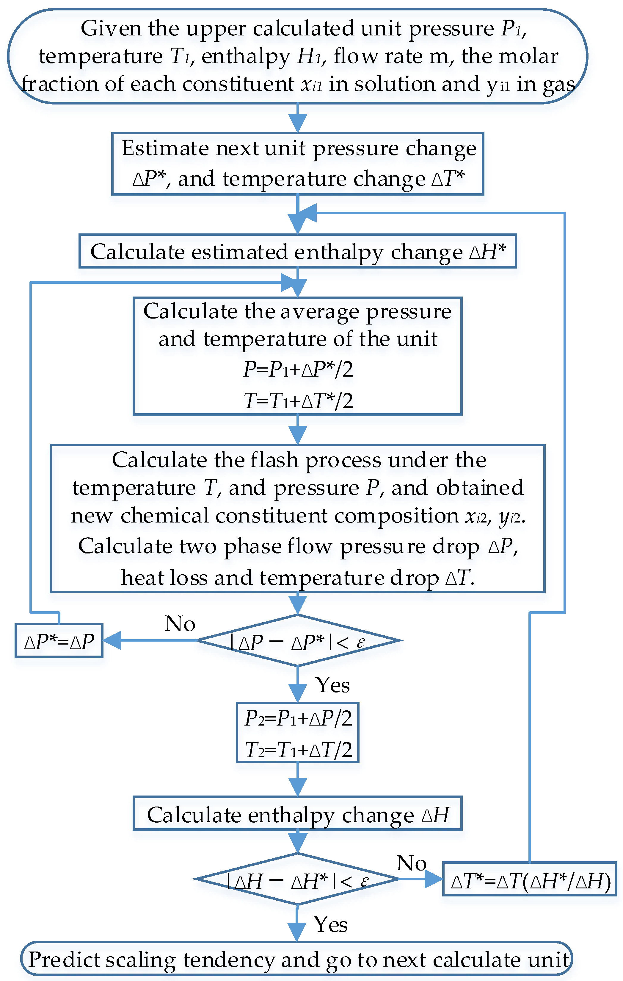
2.2. Model Solution Algorithm

The geothermal water flow in the interior of the wellbore is simplified as one-dimensional steady flow. The wellbore is divided into many computational units in the length direction and the parameters of each unit are calculated step by step from the well bottom to the top, including heat transfer, fluid flow, chemical change and scaling, etc. The unit calculation flowchart is shown in Figure 2.

The flash simulation algorithm is the most complex part in this paper. Luckily, the flash separation process algorithm is a well-developed topic in the subject of chemical engineering simulation [22]. The typical method is to obtain an N + M-dimensional equation set according to the relationship between ionization balance and phase balance for a two-phase system containing N components (all ions and molecules) and M chemical reactions, such as ionization or hydrolysis. The nonlinear equations are solved by Marquardt iterative algorithm.

At the end of the calculation of each unit, the saturation index is calculated to determine whether scaling occurs. If scaling occurs, a certain amount will be precipitated to make the solution return to the saturation state under the current conditions, so as to obtain the balance relationship of each component.

2.3. Chemical Reaction Equations and Phase Change Equilibrium Equations

Due to the complex chemical composition of geothermal fluids, it is impossible to cover all of them. The purpose of this paper is to describe the simulation method of CaCO₃ scaling. Currently, only the interaction of CaCO₃, CO₂, H₂O, NaCl and CH₄ is considered in the wellbore scaling simulation program as shown in

Table 1. Chemical reaction and phase change equilibrium equations involved in this simulation program.

No.	Equations
1	${\mathrm{H}}_2\mathrm{O}+{\mathrm{CO}}_{2(\mathrm{aq})}\leftrightarrow {\mathrm{HCO}}_3{}^{-}+{\mathrm{H}}^{+}$
2	${\mathrm{HCO}}_3{}^{-}\leftrightarrow {\mathrm{CO}}_3{}^{2-}+{\mathrm{H}}^{+}$
3	${\mathrm{H}}_2\mathrm{O}\leftrightarrow {\mathrm{H}}^{+}+{\mathrm{OH}}^{-}$
4	${\mathrm{CaHCO}}_3{}^{+}\leftrightarrow {\mathrm{Ca}}^{2+}+{\mathrm{HCO}}_3{}^{-}$
5	${\mathrm{CaCO}}_3{}^0\leftrightarrow {\mathrm{Ca}}^{2+}+{\mathrm{CO}}_3{}^{2-}$
6	${\mathrm{Ca}\left(\mathrm{OH}\right)}^{+}\leftrightarrow {\mathrm{Ca}}^{2+}+{\mathrm{OH}}^{-}$
7	${\mathrm{H}}_2{\mathrm{O}}_{\left(\mathrm{aq}\right)}\leftrightarrow {\mathrm{H}}_2{\mathrm{O}}^{\mathrm{g}}$
8	${\mathrm{CO}}_{2(\mathrm{aq})}\leftrightarrow {\mathrm{CO}}_2{}^{\mathrm{g}}$
9	${\mathrm{NaCl}}^{\mathrm{s}}(\mathrm{halite})\leftrightarrow {\mathrm{Na}}^{+}+{\mathrm{Cl}}^{-}$
10	${\mathrm{CaCO}}_3{}^{\mathrm{s}}(\mathrm{calcite})\leftrightarrow {\mathrm{Ca}}^{2+}+{\mathrm{CO}}_3{}^{2-}$
11	${\mathrm{CH}}_{4(\mathrm{aq})}\leftrightarrow {\mathrm{CH}}_4{}^{\mathrm{g}}$

Note: the subscript aq refers to solution, ^g refers to gas phase and ^s refers to solid phase.

.

2.4. Programming

The wellbore simulation program is written in the Visual Studio 2019 integrated development environment with Python computer language. Tkinter library is used to make a simple parameter input interface. Then, one can easily input the parameters of each example.

3. Field Test for Prediction of the Depth of the First Gas Bubble or Scaling of a Real Geothermal Well

3.1. The Situation of the Tested Geothermal Well

The geothermal well selected in the test is located in Boye County, Hebei Province, China (as shown in Figure 3). This area is located within the hinterland of Jizhong Plain, the middle of Hebei Province and 50 km south of Baoding city. The tectonic position of this area is located in the east-central margin of North China Plate (level 1), Bohai Bay Basin (level 2), Jizhong Depression (level 3), Gaoyang low uplift (level 4 tectonic unit) and the junction of Gaoyang low uplift and Raoyang depression. According to the rock debris logging, drilling time (speed) logging and comprehensive logging data, combined with the comparative analysis of regional geological information, the geothermal well drilled from top to bottom encountered Quaternary Pingyuan Formation, Upper Tertiary Minghuazhen Formation, Guantao Formation, Dongying Formation, Lower Tertiary Shahejie Formation, Kongdian Formation and Wumishan Formation (not drilled through).

The well has a shape of three-stage structure. Three kinds of seamless petroleum steel tubes are used with different well diameters. The well structure for fluid flow is formed as shown in

Table 2. Well structure.

Depth (m)	Inner Diameter (mm)
0~462	320.4
462~3056	226.62
3056~3570	159.42

. The well is currently used for heating in the residential area and the submersible pump is put into the well at a depth of 110 m. The roughness of the tube is about 0.015 mm.

3.2. Field Test Methods

(1)

The depth of scaling:

Open the tube at the wellhead and observe visually.

(2)

Static temperature and pressure of the well:

Professional logging truck is used to measure static wellbore pressure and temperature data. Temperatures and pressures every 10 m from wellhead to the well bottom are recorded and saved in an Excel spreadsheet.

(3)

Gas and liquid chemical composition analysis of the geothermal water:

A sampling port is set at the wellhead. After gas–liquid separation, the gas and liquid are sampled, respectively. The gas composition and contents are analyzed by gas chromatography. The composition of the water sample was sent to professional institutions for analysis. After filtration, the geothermal water is analyzed by induced plasma mass spectrometer, titration and ion chromatography.

(4)

Measuring method of noncondensable gas contents in a unit weight of geothermal water:

A drainage method is used to measure the noncondensable gas content in geothermal water. As shown in Figure 4, the testing procedure is as follows.

At first, the volume of water in a bucket was recorded. Then, a bottle filled with the water was turned upside down in the bucket with the bottle mouth submersed in the water (Figure 4a). In the second step, the valve was opened and the geothermal water containing noncondensable gas flowed into the bottle. As a result, the noncondensable gas was collected inside the bottle (Figure 4b). In the third step, the valve was closed after collecting a certain amount of gas. When the water temperature was equal to the ambient temperature after a while or was the ambient temperature, T was recorded. The bottle was moved up and down to make the liquid surface inside and outside the bottle reach the same level (Figure 4c), so that the pressure of the gas in the bottle is equal to 1 atm. The volume of the gas at this time V was recorded (after making a record and drawing a line on the bottle, use a measuring cylinder to measure the volume with water), then the increased geothermal water m was measured by a measuring cylinder. According to the following equation, the molar of noncondensable gas n can be calculated.

$$(P-P_{\mathrm{water},\mathrm{s}}(T))V=nRT$$

(22)

where P is 1 atm; T is ambient temperature in K; P_water,s is water saturated pressure under the ambient temperature; R is universal gas constant. Then, n/m is the noncondensable gas content in a unit weight of geothermal water.

(5)

Measurement of the total mass flow rate of the geothermal water:

The total mass flow rate of the geothermal water is measured by an ultrasonic flowmeter.

(6)

Measurement of the dynamic temperature and pressure at the wellhead:

A mechanical temperature meter with an accuracy of ±1.0% and a mechanical pressure meter with an accuracy of ±1.6% are fixed in the wellhead and we can read the real-time data.

4. Results and Discussion

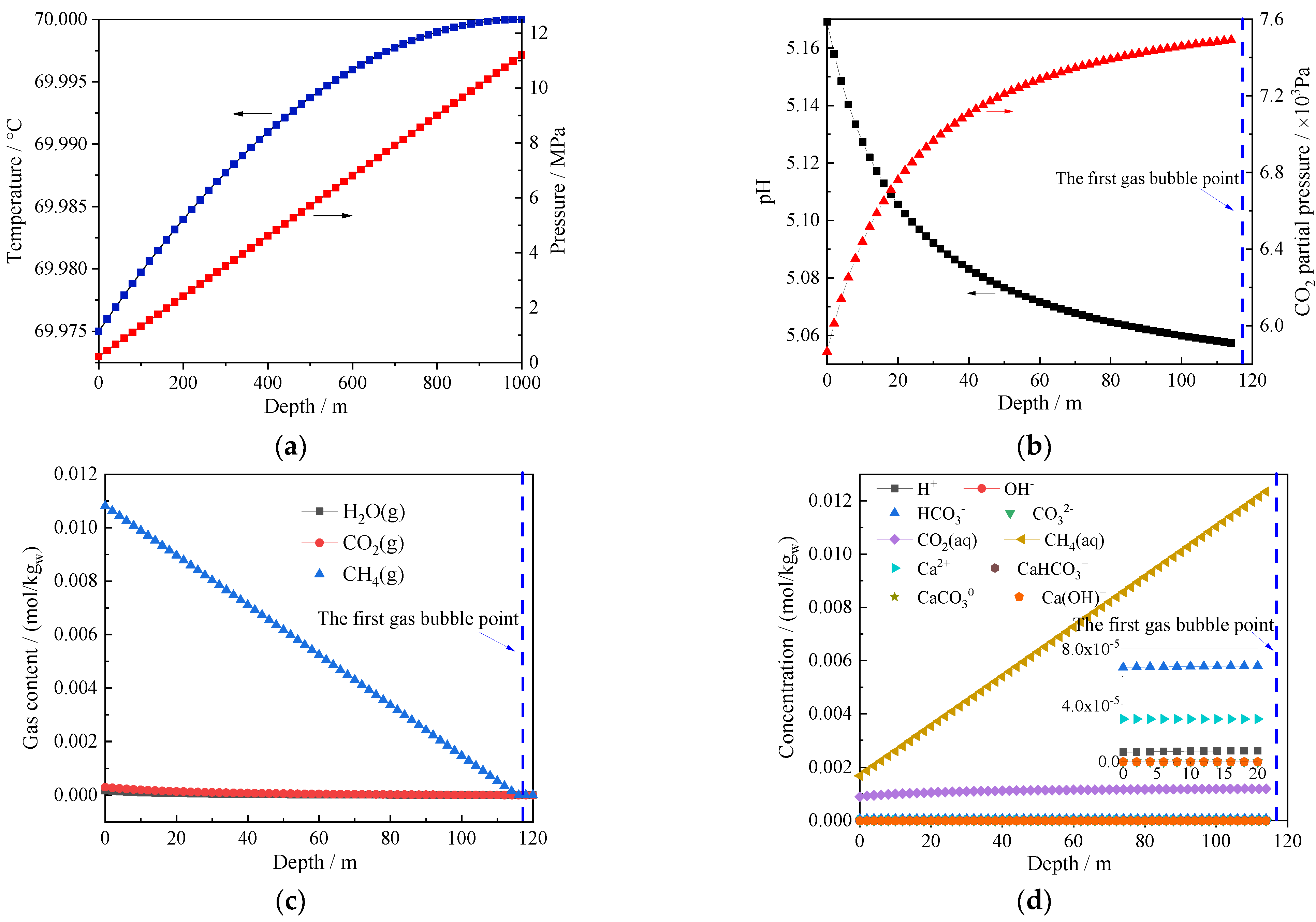
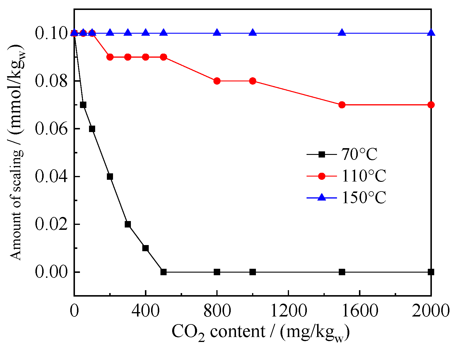
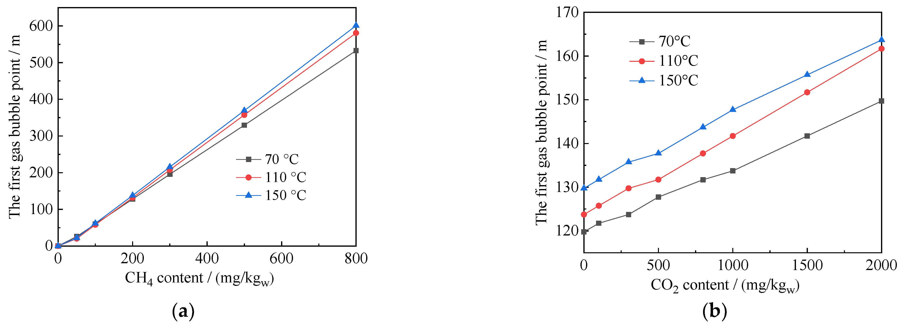
4.1. Analysis of a Trial Computation

Example input parameters are shown in

Table 3. Example input parameters.

Item	Value
Total depth of the wellbore	1000 m
Inner diameter	200 mm
Pipe inner surface roughness	0.015 mm
Bottom hole temperature	70 °C
Bottom hole pressure	11.2 MPa
Flow rate	2.5 kg/s
Ca2+ content	4.0 mg/kgw
HCO3− content	12.18 mg/kgw
CO2 content	50 mg/kgw
CH4 content	200 mg/kgw
ground surface temperature	25 °C

. The Earth formation temperature is calculated as a linear change from ground surface to bottom hole.

The wellbore is divided into 500 computational sections (optional) and parameters, such as gas–liquid component composition, temperature, pressure, flow rate, pH and scaling saturation index, of each unit are obtained after calculation by simulation program, as shown in

Table 4. Concentration of each component in the geothermal water at different depths of the well.

Condition	Concentration/(mol/kgw)
h = 1 000 m T = 343.15 K P = 112.0 bar	H+	OH−	HCO3−	CO32−	CO2(aq)	CH4(aq)	Ca2+
	2.84 × 10−6	5.90 × 10−8	2.02 × 10−4	5.47 × 10−9	1.13 × 10−3	1.25 × 10−2	9.93 × 10−5
	CaHCO3+	CaCO30	Ca(OH)+	H2O(aq)	H2O(g)	CO2(g)	CH4(g)
	4.81 × 10−7	3.52 × 10−9	2.62 × 10−7	55.540 76	0.00	0.00	0.00
h = 150 m T = 342.47 K P = 18.7 bar	H+	OH−	HCO3−	CO32−	CO2(aq)	CH4(aq)	Ca2+
	2.81 × 10−6	5.53 × 10−8	2.02 × 10−4	5.44 × 10−9	1.13 × 10−3	1.25 × 10−2	9.93 × 10−5
	CaHCO3+	CaCO30	Ca(OH)+	H2O(aq)	H2O(g)	CO2(g)	CH4(g)
	4.79 × 10−7	3.42 × 10−9	2.32 × 10−7	55.540 76	0.00	0.00	0.00
h = 60 m T = 342.28 K P = 8.8 bar	H+	OH−	HCO3−	CO32−	CO2(aq)	CH4(aq)	Ca2+
	8.51 × 10−6	1.74 × 10−8	6.81 × 10−5	6.08 × 10−10	1.16 × 10−3	7.28 × 10−3	2.99 × 10−5
	CaHCO3+	CaCO30	Ca(OH)+	H2O(aq)	H2O(g)	CO2(g)	CH4(g)
	4.86 × 10−8	1.15 × 10−10	2.27 × 10−8	55.540 81	1.82 × 10−5	4.33 × 10−5	5.22 × 10−3
h = 0 m T = 342.16 K P = 2.2 bar	H+	OH−	HCO3−	CO32−	CO2(aq)	CH4(aq)	Ca2+
	6.81 × 10−6	2.15 × 10−8	6.64 × 10−5	7.40 × 10−10	9.00 × 10−4	1.68 × 10−3	2.99 × 10−5
	CaHCO3+	CaCO30	Ca(OH)+	H2O(aq)	H2O(g)	CO2(g)	CH4(g)
	4.74 × 10−8	1.39 × 10−10	2.80 × 10−8	55.540 67	1.6 × 10−4	3.00 × 10−4	1.08 × 10−2

Note: the subscript aq refers to solution, g refers to gas phase.

. The partial pressure of each kind of gas is the total pressure multiplied by its gas phase mole fraction and fugacity coefficient. The pH can be determined by H⁺ concentration. The cumulative scale of CaCO₃(s) is 7.0 × 10⁻⁵ mol/kg_w. The depth of the first gas bubble or initial scaling point is 118 m. Therefore, the four representative depths in Table 4 are the bottom of the well, the wellhead, the point before the bubble point (150 m) and the point after the bubble point (60 m), respectively. They are selected to show how parameters change along the wellbore.

Figure 5 is the output data of the calculation example. Figure 5a shows the curves of temperature and pressure changes along the well. Figure 5b–d show evolutions of geothermal water pH, partial pressure of CO₂ and composition of gas and liquid phases after the first gas bubble point, respectively. Under a mass flow rate of 2.5 kg/s flow rate, the temperature decrease is small and the pressure decreases linearly. After the first gas bubble point, due to the escape of CO₂, the pH of geothermal water increases exponentially and the partial pressure of CO₂ decreases rapidly. These curve evolution trends match the calcite scaling mechanism very well. The change in gas composition in Figure 5c shows that CH₄ gas has a faster growth rate than CO₂, because CH₄ has a lower solubility in water. Figure 5d shows the change in concentration of each component in the liquid phase. It can be seen that, except for free CO₂ molecules, CH₄ molecules, HCO³⁻ and Ca²⁺, the concentration of other components in the solution is low, less than 1 × 10⁻⁵ mol/kg_w. In other words, calculated parameters changed significantly after the first gas bubble point, while they were almost unchanged before the first gas bubble point, except for the total pressure.

Effects of Noncondensable Gas on the First Gas Bubble Point and Scale

Figure 6 shows the variation curves of the ultimate scale amount, changing with CO₂ content under different well bottom temperatures. This was achieved by changing the two variables of well bottom temperature and CO₂ content based on the above calculation example. The final amount of scale is calculated by keeping CaCO₃ saturation index less than zero. As can be seen from the figure, under a well bottom temperature of 70 °C, the amount of scale decreases with an increase in CO₂ content and, when the CO₂ content reaches a certain level, the amount of scale approaches 0. Under the same CO₂ content, with an increase in well bottom temperature, the amount of scale increases, but due to the limitation of Ca²⁺, the amount of scale also is limited to a certain maximum.

Figure 7 shows the influence of CH₄ and CO₂ content per kg of geothermal water on the depth of the first gas bubble under the above calculation example conditions. It can be seen from the figure that the depth of the first gas bubble is linearly increased with the content of these two noncondensable gases. In general, the depth of the first gas bubble is the location where scaling begins. As the content of noncondensable gases increases, the gases escape more easily from the aqueous solution and the flash point becomes deeper.

4.2. Field Test Results

(1)

The position of scale is right at the wellhead.

(2)

The logging truck results were recorded in an Excel spreadsheet that recorded temperature and pressure data points every 10 m. Part of the data is shown in

Table 5. Static temperature and pressure in the tested well.

Depth (m)	Temperature (°C)	Gage Pressure (MPa)
72	23.377	0
1000	65.356	8.988
2000	102.649	18.479
3000	137.52	27.72
3570	142.937	32.89

. The static water surface is at a depth of 72 m. The temperature and pressure of the geothermal water in the bottom of the well (depth of 3570 m) are 142.937 °C and 32.89 MPa, respectively.

(3)

The analysis and test center of Guangzhou Institute of Energy Conversion, Chinese Academy of Sciences, detected that the main components of noncondensable gas are 90% CO₂ and 10% CH₄. The liquid composition was tested by the Groundwater Mineral Water and Environment Monitoring Center of the Ministry of Land and Resources, China, and the results are shown in

Table 6. Concentration of each constituent in the geothermal water.

Constituent	K+	Na+	Ca2+	Mg2+	HCO3−	CO32−	Cl−	SO42−	F−	NO3−
Concentration (mg/kgw)	200.6	1889	79.95	12.36	579.1	100.0	2757	116.1	8.35	1.62

.

(4)

The noncondensable gas content in a unit weight of geothermal water is 0.003668 mol/kg_w.

(5)

The total mass flow rate of the geothermal water is 90 m³/h.

(6)

The temperature is 121 °C and pressure is 3.5 bar at the wellhead.

4.3. Depth Prediciton of the First Gas Bubble by Wellbore Simulation

Putting the field test data above into the wellbore simulation program described in Section 2, the depth of the first gas bubble or scale starting point can be predicted. In this well, a submerged pump is placed at a depth of 110 m. In our simulation model, the pressure of the geothermal water is increased suddenly by a certain pressure boost according to the performance of the pump. The lift of the submerged pump is 19 m at a total mass flow rate of 90 m³/h. Geothermal water flows into the pump pipe with a diameter of 150 mm after the pump.

The temperature of the formation for each calculation section is obtained by using linear interpolations between tabulated data from the logging truck. For chemical components that are not considered in the program, anions are subsumed with Cl⁻ input of equal mole charge and cations with Na⁺ input of equal mole charge. For example, 1 mol SO₄²⁻ can be regarded as 2 mol Cl⁻ and 1 mol K⁺ ion can be regarded as 1 mol Na⁺ ion for calculation.

As the well bottom pressure will decrease during the dynamic flow of geothermal wells, the magnitude of the pressure drop factor is related to the formation permeability and other geological properties and, usually, is not easy to obtain. The well bottom pressure under a dynamic condition can be continuously adjusted by multiple trial calculations and after the calculations, the appropriate value can be obtained by comparing with the real wellhead pressure. Similarly, in the process of heat dissipation calculation, the actual formation thermal conductivity k_e is also not easy to obtain. If it cannot be provided, some estimated values can be set and several trial calculations carried out until the well bottom temperature and wellhead temperature are consistent with the measured data. After obtaining satisfactory results, the depth of the first gas bubble can be calculated at about 2 m, which is consistent with the actual location of scaling at the wellhead.

Although we take the geothermal well in Boye county, Hebei Province, China, as an example to show the prediction of the scaling procedure, the methods are suitable to all geothermal wells involving the calcite scaling problem. For other type of scales, other chemical component properties are needed to add into equations of chemical reaction equilibrium manually. However, the computational algorithm is the same. Following the procedure described above, one can easily estimate the depth of the scaling in the geothermal well without reservoir parameters that are hard to obtain.

5. Conclusions

In this paper, models of two-phase flow, chemical reaction equilibrium and flashing are combined together to simulate the flow in a geothermal well. The simulation is able to obtain the change in temperature, pressure, chemical components in the gas and liquid phase, pH and gas phase partial pressure, determine the depth of the first gas bubble and judge the tendency of scaling, etc. A simple calculation example shows that the numerical results are reasonable. It can establish the exponential decrease in CO₂ partial pressure and exponential increase in pH after the occurrence of the first gas bubble. At the same time, after parameter sensitivity analysis, the following three conclusions can be drawn: (1) with an increase in CO₂ content, the amount of scaling gradually decreases until no scaling occurs; (2) the higher the geothermal water temperature, the more likely scaling is to occur; (3) with an increase in noncondensable gas, the first gas bubble location, that is, the scaling location, becomes deeper.

The chemical composition of geothermal water in the simulation program of this paper only includes Ca²⁺, HCO³⁻, Na⁺, Cl⁻ ions and CO₂, CH₄ noncondensable gases. However, real geothermal brine contains more complex components. More chemical components can be added on the basis of this model framework. By using appropriate chemical constants, such as a chemical reaction equilibrium constant and Henry coefficient, the real flow and chemical change in a geothermal well can be accurately simulated.

Based on the simulation model, this paper discusses, in detail, the field test data acquisition process and computational prediction procedure for the scale location of geothermal wells containing noncondensable gases. Through drainage and liquid surface-level balance methods, noncondensable gas content in the geothermal water can be measured. When inputting chemical composition into the simulation program, chemical components not mentioned in the program are combined with corresponding similar components that are already considered. While it is difficult to obtain the bottom hole pressure drop factor and the actual Earth formation thermal conductivity directly, repeated calculation and comparison with the well bottom temperature and pressure are carried out to figure them out indirectly. The depth of the first gas bubble resulting from the simulation program is very close to the location of scaling detected in the field.

References

1. Yanagisawa, N.; Matsunaga, I.; Sato, M.; Okabe, T. Temperature-dependent scale precipitation in the Hijiori Hot Dry Rock system, Japan. Geothermics 2008, 37, 1–18. [Google Scholar] [CrossRef]
2. Pauwels, J.; Salah, S.; Vasile, M.; Laenen, B.; Cappuyns, V. Characterization of scaling material obtained from the geothermal power plant of the Balmatt site. Mol. Geotherm. 2021, 94, 102090. [Google Scholar] [CrossRef]
3. Tonkul, S.; Baba, A.; Demir, M.M.; Regenspurg, S. Characterization of Sb scaling and fluids in saline geothermal power plants: A case study for Germencik Region (Büyük Menderes Graben, Turkey). Geothermics 2021, 96, 102227. [Google Scholar] [CrossRef]
4. Zolfagharroshan, M.; Khamehchi, E. A rigorous approach to scale formation and deposition modelling in geothermal wellbores. Geothermics 2020, 87, 101841. [Google Scholar] [CrossRef]
5. Zhang, Y.P.; Shaw, H.; Farquhar, R.; Dawe, R. The kinetics of carbonate scaling—Application for the prediction of downhole carbonate scaling. J. Petrol. Sci. Eng. 2001, 29, 85–95. [Google Scholar] [CrossRef]
6. Haklıdır, F.S.T.; Balaban, T.Ö. A review of mineral precipitation and effective scale inhibition methods at geothermal power plants in West Anatolia (Turkey). Geothermics 2019, 80, 103–118. [Google Scholar] [CrossRef]
7. Zhang, L.; Geng, S.H.; Chao, J.H.; Yang, L.C.; Zhao, Z.; Qin, G.X.; Ren, S.R. Scaling and block risk in geothermal reinjection wellbore: Experiment assessment and model prediction based on scaling deposition kinetics. J. Petrol. Sci. Eng. 2022, 209, 109867. [Google Scholar] [CrossRef]
8. Song, J.C.; Liu, M.Y.; Sun, X.X. Model analysis and experimental study on scaling and corrosion tendencies of aerated geothermal water. Geothermics 2020, 85, 101766. [Google Scholar] [CrossRef]
9. Wang, Y.X.; Liu, S.L.; Bian, Q.Y.; Yan, B.; Liu, X.F.; Liu, J.X.; Wang, H.Y.; Bu, X.B. Scaling analysis of geothermal well from Ganzi and countermeasures for anti-scale. Adv. New Renew. Energ. 2015, 3, 202–206. (In Chinese) [Google Scholar] [CrossRef]
10. Liu, M.Y. A review on controls of corrosion and scaling in geothermal fluids. Adv. New Renew. Energy 2015, 3, 38–46. (In Chinese) [Google Scholar] [CrossRef]
11. Zhu, J.L.; Yao, T. Judgement and calculation of trend of corrosion and scaling of geothermal water. Ind. Water Waste Water 2004, 35, 23–25. Available online: https://www.docin.com/p-842500009.html (accessed on 1 October 2022). (In Chinese).
12. Haklidir, F.T.; Haklidir, M. Fuzzy control of calcium carbonate and silica scales in geothermal systems. Geothermics 2017, 70, 230–238. [Google Scholar] [CrossRef]
13. Topcu, G.; Koç, G.A.; Baba, A.; Demir, M.M. The injection of CO2 to hypersaline geothermal brine: A case study for Tuzla region. Geothermics 2019, 80, 86–91. [Google Scholar] [CrossRef]
14. Zhang, H.; Hu, Y.Z.; Yun, Z.H.; Qu, Z.W. Applying hydro-geochemistry simulating technology to study scaling of the high-temperature geothermal well in Kangding County. Adv. New Renew. Energy 2016, 4, 111–117. (In Chinese) [Google Scholar] [CrossRef]
15. Haizlip, J.R.; Guney, A.; Haklıdır, F.S.T.; Garg, S.K. The Impact of High Noncondensible Gas Concentrations on Well Performance Kizildere Geothermal Reservoir, Turkey. In Proceedings of the Thirty-Seventh Workshop on Geothermal Reservoir Engineering, Stanford, CA, USA, 30 January–1 February 2012; SGP-TR-194. Available online: http://www.researchgate.net/profile/Fusun_Tut_Haklidir/publication/250928326_THE_IMPACT_OF_HIGH_NONCONDENSIBLE_GAS_CONCENTRATIONS_ON_WELL_PERFORMANCE_KIZILDERE_GEOTHERMAL_RESERVOIR_TURKEY/links/00b7d51ee5d013cfe7000000 (accessed on 1 October 2022).
16. Akin, T.; Güney, A.; Kargi, H.; Haklıdır, T.; Garg, S.K. Modeling of calcite scaling and estimation of gas breakout depth in a geothermal well by using PHREEQC. In Proceedings of the Fortieth workshop on Geothermal Reservoir Engineering, Stanford, CA, USA, 26–28 January 2015; SGP-TR-204. Available online: https://www.researchgate.net/profile/Taylan-Akin-3/publication/272483835_MODELING_OF_CALCITE_SCALING_AND_ESTIMATION_OF_GAS_BREAKOUT_DEPTH_IN_A_GEOTHERMAL_WELL_BY_USING_PHREEQC/links/54e59eaf0cf276cec1746f2c/MODELING-OF-CALCITE-SCALING-AND-ESTIMATION-OF-GAS-BREAKOUT-DEPTH-IN-A-GEOTHERMAL-WELL-BY-USING-PHREEQC.pdf (accessed on 1 October 2022).
17. Pátzay, G.; Stáhl, G.; Kármán, F.H.; Kálmán, E. Modeling of scale formation and corrosion from geothermal water. Electrochim. Acta 1998, 43, 137–147. [Google Scholar] [CrossRef]
18. Pátzay, G.; Kármán, F.H.; Póta, G. Preliminary investigations of scaling and corrosion in high enthalpy geothermal wells in Hungary. Geothermics 2003, 32, 627–638. [Google Scholar] [CrossRef]
19. Liang, H.J.; Guo, X.F.; Gao, T.; Bu, X.B.; Li, H.S.; Wang, L.B. Scaling spot prediction and analysis of influencing factors for a geothermal well in Boye County, Hebei Province. Petrol. Drilling Tech. 2020, 48, 105–110. (In Chinese) [Google Scholar] [CrossRef]
20. Hasan, A.R.; Kabir, C.S. Modeling two-phase fluid and heat flows in geothermal wells. J. Petrol. Sci. Eng. 2010, 71, 77–86. [Google Scholar] [CrossRef]
21. Garg, S.K.; Pritchett, J.W.; Alexander, J.H. A new liquid hold-up correlation for geothermal wells. Geothermics 2004, 33, 795–817. [Google Scholar] [CrossRef]
22. Han, S.S. Research and Development of PROCESS Simulation Containing Electrolyte. Master’s Thesis, Qingdao University of Science and Technology, Qingdao, China, 2019. Available online: https://d.wanfangdata.com.cn/thesis/D01733218 (accessed on 1 October 2022). (In Chinese).
23. Minkowycz, W.J.; Cheng, P. Free convection above a circular cylinder embedded in a porous medium. Int. J. Heat Mass Transf. 1976, 19, 805–813. [Google Scholar] [CrossRef]
24. Pritchett, J.W. Preliminary study of discharge characteristics of slim holes compared to production wells in liquid-dominated geothermal reservoirs. In Proceedings of the 18th Workshop Geothermal Reservoir Engineering, Stanford, CA, USA, 26–28 January 1993; pp. 181–187. [Google Scholar] [CrossRef]
25. Pitzer, K.S. Electrolytes from diluted solutions to fuse salts. J. Am. Chem. Soc. 1980, 102, 2902–2906. [Google Scholar] [CrossRef] [Green Version]
26. Li, J.; Wei, L.L.; Li, X.C. Modeling of CO2-CH4-H2S-brine based on cubic EOS and fugacity-activity approach and their comparisons. Energy Procedia 2014, 63, 3598–3607. [Google Scholar] [CrossRef]
Figure 1. Schematic of phase equilibrium model of electrolyte solution.
Processes 10 02018 g001
Figure 2. Flow chart of a calculation unit.
Processes 10 02018 g002
Figure 3. Location of Boye County, Heibei province, China.
Processes 10 02018 g003
Figure 4. Schematic of noncondensable gas content measuring steps: (a) turn a bottle upside down filled with water; (b) open the valve let geothermal fluid flow inside the bottle; (c) move the bottle to make the liquid surface inside and outside the bottle is at the same level.
Processes 10 02018 g004
Figure 5. (a) Temperature and pressure distribution along the well; (b) CO2 partial pressure and pH evolution after the first gas bubble point; (c) concentration evolution of gas components after the first gas bubble point; (d) concentration evolution of liquid components after the first gas bubble point.
Processes 10 02018 g005
Figure 6. Relation of scale quantities with CO2 content under different well fluid temperatures.
Processes 10 02018 g006
Figure 7. The effect of CH4 (a) and CO2 (b) contents on the first gas bubble point.
Processes 10 02018 g007