An Overview of Molecular Dynamics Simulation for Food Products and Processes

Abstract

Molecular dynamics (MD) simulation is a particularly useful technique in food processing. Normally, food processing techniques can be optimized to favor the creation of higher-quality, safer, more functional, and more nutritionally valuable food products. Modeling food processes through the application of MD simulations, namely, the Groningen Machine for Chemical Simulations (GROMACS) software package, is helpful in achieving a better understanding of the structural changes occurring at the molecular level to the biomolecules present in food products during processing. MD simulations can be applied to define the optimal processing conditions required for a given food product to achieve a desired function or state. This review presents the development history of MD simulations, provides an in-depth explanation of the concept and mechanisms employed through the running of a GROMACS simulation, and outlines certain recent applications of GROMACS MD simulations in the food industry for the modeling of proteins in food products, including peanuts, hazelnuts, cow’s milk, soybeans, egg whites, PSE chicken breast, and kiwifruit.

1. Introduction

The motivation behind and technology applied in food processing have dramatically changed over humanity’s history, often based on the socio-economic context of the time [1]. Currently, modern processing techniques are most commonly applied to improve the safety, shelf life, convenience, and nutritional, functional, and organoleptic qualities of processed food products [2]. Food processes no longer only involve treatment by conventional thermal, chemical, or mechanical means but may equally include novel treatment methods utilizing high hydrostatic pressure, radiation, microwaves, ultrasound, pulsed electric fields, or cold plasma [3]. Understanding the consequences that the application of these external stressors has on the biomolecules present in food products, namely, the carbohydrates, proteins, and lipids, is critical in determining optimal processing conditions. This is where food process engineering is involved, as its primary goal is to better understand the process in order to better manipulate it [4]. By better controlling food processes, a more desirable finished product that better meets the population’s needs can be offered. Although this is easily said, this, in reality, is no simple task, seeing as food processes are often dynamic and involve highly complex mechanisms [4]. Simulation modeling is an important tool that helps to bridge this gap, as it actively combines knowledge of physics, statistics, applied mathematics, and computing to predict the result of a given processing treatment with sufficient accuracy for the application [4,5]. The development of an accurate mathematical model that simulates the real-life mechanism with minimal data noise can eliminate the need for repetitive, isolated experimental trials [5]. It can equally allow for continuous improvement and learning, while also serving to improve experimental design efficiency, thus limiting costs and time invested [5].

One such computational methodology is the use of atomistic molecular dynamics (MD) simulation. Atomistic MD simulation is, at its core, based on Newton’s equation of motion [6]. Each atom, part of the molecular system being modeled, is assigned a position vector defined as a function of time [6]. This position vector then fluctuates based on the stresses acting on the atom through time [6]. The stresses that can be applied to each atom include any relevant forces, originating from “inter-atomic interactions, [treatment] energy and interactions between the molecular system and [its] environment”, namely, the presence of water or salt molecules [6]. Near the end of the 1950s, the concept of molecular dynamics was initially proposed by two physicists, Berni Alder and Tom Wainwright, who were studying statistical mechanics at Lawrence Radiation Laboratory in Livermore, California [7]. Molecular dynamics was a substitute for the earlier Monte Carlo simulation [7]. In a time where few physicists and chemists trusted computer simulations over traditional theoretical methods, Alder and Wainwright were able to successfully model, using both molecular dynamics simulation and Monte Carlo, the interactions and consequent phase transition in a hard-sphere generic molecular system [7]. Later, between 1960 and 1970, other researchers applied MD simulation to model increasingly realistic material systems, including solid copper and liquid argon [8]. However, in September 1974, chemist Frank Stillinger and physicist Aneesur Rahman refined this initial model to simulate the molecular interactions of liquid water molecules at four different temperatures [9]. McCammon et al. [10] further expanded the applications of MD simulation, running a 9.2-picosecond simulation of the dynamics of a small, folded globular protein, a bovine pancreatic trypsin inhibitor held in vacuum. The same study was reworked eleven years after with the bovine trypsin inhibitor now solvated in water, and an improved simulation length of 210 picoseconds was achieved [11].

Since then, with the increasing availability of computing power, simulation lengths of MD simulations have increased dramatically to between 10 and 300 nanoseconds for increasingly long polypeptide chains [11,12]. Currently, polished atomistic MD simulations are being applied in a variety of domains for the modeling of diverse biological molecules, namely, DNA, RNA, and proteins [6]. Atomistic MD simulations have been routinely applied in the pharmaceutical industry for drug discovery and drug design [13]. However, in recent years, they have been increasingly applied in food process engineering to provide greater insight into the molecular interactions and consequent conformational and functional property changes that take place during the processing of food products [2]. The effect of food processes on the structure and function of food carbohydrates, lipids, and other small molecules has been investigated using MD simulations [14]. However, recent emphasis has been placed on MD simulations of food proteins, due to their unique properties, including their diverse conformational states, ability to denature and unfold, ability to interact among themselves and with other biomolecules, their important influence on the functional properties of the foods they are present in, and their capacity to function as an enzyme [14]. Proteins not only play a vital nutritional role in the body following their consumption, but they equally confer certain dynamic functional properties to the food products themselves prior to consumption [15]. Protein structure, which dictates the protein’s function, may influence viscosity, texture, emulsification, gelation, and water absorption and retention. It has equally been suggested that changes in proteins’ conformational state, notably their surface area, limits access to allergenic epitopes, which, when in contact with a T cell or immunoglobulin E antibody, cause allergic reactions by the immune system [16].

Studies targeting food proteins that have already utilized atomistic MD simulations include Ara h 6 in peanuts [17], trypsin inhibitor in soybean [18], bovine β-lactoglobulin in cow’s milk [16], profilin in hazelnuts [12], Act d 2 in kiwifruit [19], avidin in egg whites [20], and myofibrillar proteins in pale, soft, exudative chicken breast meat [21]. MD simulations have equally been employed to simulate the effects of diverse food processes, including the application of thermal and electric fields, both static and oscillating [17]. Although MD simulations have currently only been utilized for a restricted set of food proteins to study the effect of only a couple of food processes, atomistic MD simulations offer potentially endless possibilities, as there is vast opportunity for continued research in this field. This review article provides a general overview of the Groningen Machine for Chemical Simulations (GROMACS) software package for running MD simulations of food proteins and presents the current and potential future applications of MD simulations using GROMACS, along with its most prominent barriers to implementation.

2. GROMACS Software Package for Molecular Dynamics Simulation

Proteins are omnipresent and highly complex macromolecules made up of polypeptide chains [22]. The polypeptide chains that form proteins are composed of many successive amino acid subunits linked together by peptide bonds, which are formed through a simple dehydration reaction [22]. The three-dimensional conformation and protein–protein interactions characteristic of many polypeptides are widely classified into four distinct categories, including primary, secondary, tertiary, and quaternary structures [22]. The primary and secondary structures of proteins refer to the specific amino acid sequence of a polypeptide and the folding of that amino acid chain into α-helices and β-sheets, respectively [22]. The tertiary structure then considers the three-dimensional shape of the protein, including the secondary folding and any other turns or coils held by weak interactive forces [22]. Finally, given the ability of multiple polypeptide chains to aggregate together, the quaternary structure takes into consideration their joint spatial arrangement [22]. Ultimately, these four components of protein structure dictate the protein’s final function [15]. For this reason, being able to accurately model the protein’s conformational states over time, with enough precision to be able to visualize the molecular details of the system, is critical in achieving a better understanding of the macroscopic behavior of a food product during processing [2].

Groningen Machine for Chemical Simulations (GROMACS) is an extremely valuable, fast, free, user-friendly, and high-performing molecular dynamics software package, created at the University of Groningen in the Netherlands [23]. It allows users to develop a virtual molecular model of up to millions of atoms that simulates highly complex biomolecules, to which Newton’s equation of motion can then be applied [23]. The GROMACS software package is composed of three distinct programs: “a preprocessor, a parallel MD and an energy minimization program” [23]. In response to growing research interests, the GROMACS software is constantly being reworked to improve flexibility, provide better handling of errors, and minimize simulation run times [23]. GROMACS was initially programmed using the C programming language but has recently incorporated certain sections of code, written in C++ to improve general versatility [23]. However, it is important to note that although GROMACS offers users the unique opportunity to visualize the dynamic behavior of particles in larger macromolecules under stress, it is only suitable for “the verification of physical principles, which are visually prominent at the macroscale” [23], meaning that, in order to ascertain the true accuracy of any simulation, results must be confirmed against equivalent experimental data.

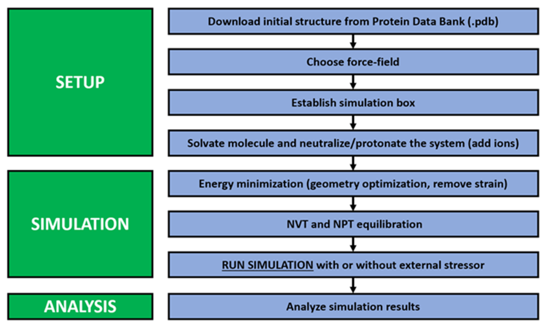
Running an effective GROMACS simulation, to supplement one’s understanding of complementary experimental data, is typically undertaken in a series of sequential steps, as depicted in Figure 1 below. The procedure for completing a GROMACS simulation is generally subdivided into three larger stages: the physical setup, the simulation, and the analysis of the obtained simulation results [14]. In order to obtain simulation results that accurately reflect experimentally derived data, each of these three steps must be thought through and performed fastidiously. The setup of the simulation first begins with the retrieval of the biomolecule’s three-dimensional structure file from the Protein Data Bank (PDB) [2]. Practically speaking, this initial structure file serves to simplify the larger biomolecule into a series of charged points or balls, each imitating a sole atom in the biomolecule’s structure and connected by deformable interatomic bonds, equated to springs [2]. This simplification of the macromolecule’s structure allows for the application of molecular dynamics. The PDB is an open access resource, amassing more than 1 terabyte of structure data for proteins, RNA, and DNA [24]. Although the PDB offers access to a wide array of biomolecular structure data, it still remains possible that the starting coordinates for one’s target molecule may not be available on the PDB. If the structure is not available for download from the PDB, the researcher may proceed by building, from scratch, their own initial structure using computational packages, including ChemOffice and PRODRG [14,25].

The next steps in setting up the simulation require the selection and application of an appropriate force field [2]. Some examples of possible force fields supported by GROMACS include Assisted Model Building and Energy Refinement (AMBER), Chemistry at Harvard Macromolecular Mechanics (CHARMM), Groningen Molecular Simulation (GROMOS), and Optimized Potential for Liquid Simulations (OPLS). The chosen force field for a given simulation will heavily depend on the type of molecular system and the level of complexity required [26]. Selecting an appropriate force field is critical, as the force field is the group of mathematical expressions that will be used, through the length of the simulation, to determine the interatomic potential energy retained in the studied molecule [26]. As shown in Figure 2, the force field equally considers, through the simulation, the evolution of bonded interactions between atoms, including bond stretching, angle bending, and torsion, as well as non-bonded interactions, namely, electrostatic and van der Waals interactions [2]. The bond between two atoms in a macromolecule has a pre-defined equilibrium bond length; any fluctuation away from that equilibrium bond length is referred to as bond stretching. Similarly, for a set of three atoms bonded together at a given equilibrium bond angle, any fluctuation in that angle is termed angle bending. Finally, torsion is generated in a dihedral angle, as four atoms in different planes rotate around a central bond. AMBER, CHARMM, GROMOS, and OPLS are all classified as Class I force fields, as they only consider both these bonded and non-bonded interactions [2]. These four force fields are all suitable for the MD modeling of proteins using GROMACS [2]. It is important to note that other classes of more complex force fields do exist; they are referred to as Class II and Class III force fields. Class II force fields, unlike Class I force fields, consider a potential cross-term effect, which includes supplementary “bond-bond, angle-angle, bond-angle, bond-dihedrals, angles-angles-dihedrals, and bond-bond-dihedrals” interactions [2]. Taking into consideration these smaller-scale interactions at the interatomic level permits slightly greater overall accuracy of the potential energy present in the system.

New force field models and improved versions of past models are continually being published as weaknesses are discovered [27]. The set of current AMBER force fields, developed specifically for use with proteins, notably includes the ff14SB and ff19SB force fields [28,29]. The ff14SB force field was developed using a well-defined fitting strategy to improve upon certain assumptions that rendered the previous AMBER force field model, the ff99SB, weaker [28]. Backbone and side chain parameters for all 20 amino acids were tweaked in the ff14SB force field to improve its overall accuracy, as it better met its benchmarks during training [28]. The most recent and up-to-date AMBER force field is the ff19SB force field, which improved upon earlier assumptions made during the development of the ff14SB model, and it markedly improved amino acid backbone profiles [29]. There are many equally relevant, revised versions of the CHARMM force field available, the most recent being the CHARMM36 force field, which is a refined model of the CHARMM22/CMAP force field [30]. Best et al. [30] rigorously tested the CHARMM36 force field, after its development, assuring its accuracy and proving it to be better equipped in assessing conformational changes in molecular dynamics studies of proteins than its predecessor CHARMM22.

The general potential energy function, expressed in mathematical terms, used to determine the force field acting on the particles during a simulation is written as in Equations (1) and (2) [26]. $U(\overrightarrow{r})$ signifies the “potential energy depending on the coordinates of the N particles” [26].

$$U(\overrightarrow{r})=U_{bond-stretching}+U_{angle-bending}+U_{torsions}+U_{electrostatic}+U_{Van der Waals}$$

(1)

$$\begin{array}{c}U(\overrightarrow{r})={\displaystyle {\displaystyle \sum }_{bond-stretching}}\frac{1}{2}{k}_b{\left(r_i-r_o\right)}^2+{\displaystyle {\displaystyle \sum }_{angle-bending}}\frac{1}{2}{k}_{\theta }{\left({\theta }_i-{\theta }_o\right)}^2+{\displaystyle {\displaystyle \sum }_{torsions}}{k}_{\varnothing } \left(1+\cos \left(n_i{\varnothing }_i-{\varnothing }_o\right)\right)\\ +{\displaystyle {\displaystyle \sum }_i^{ }}{\displaystyle {\displaystyle \sum }_{j \ne i}^{ }}\frac{q_i{q}_j}{ϵr_{ij}}+{\displaystyle {\displaystyle \sum }_i^{ }}{\displaystyle {\displaystyle \sum }_{j \ne i }^{ }}4 {ϵ}_{ij} \left({\left(\frac{{\sigma }_{ij}}{r_{ij}}\right)}^{12}-{\left(\frac{{\sigma }_{ij}}{r_{ij}}\right)}^6\right)\end{array}$$

(2)

The second component required to finalize the building of the desired force field is to identify the data to be used in the aforementioned potential energy equation. Parameters are specified in the data files appended, and they will be read by the directory of the chosen force field. The Protein Data Bank (.pdb) file, a topology file, and a parameter file are all generally required. The Protein Data Bank file principally specifies the initial x, y, and z coordinates of each atom part of the system. The topology file then elaborates on the structure of the macromolecule, namely, the atom types, charge, and mass, as well as the presence of bonds, angles, and dihedrals. Finally, the parameter file specifies the values to be used for the force constants, $k_b$, $k_{\theta }$, and $k_{\varnothing }$, and other initial criteria, including the equilibrium bond length $r_o$, the equilibrium bond angle ${\theta }_o$, the reference torsion angle ${\varnothing }_o$, the minimum value for the van der Waals term ${ϵ}_{ij}$, and the radius where the van der Waals is at a minimum ${\sigma }_{ij}$ [2].

After completing the force field specification, a simulation cell is then created by applying periodic boundary conditions [23]. This is carried out to assure that the simulation is not affected by any interactions with the neighboring environment, which is typically a vacuum [23]. The created simulation box helps to limit the edge effects between the two differing domains [23]. Imposing periodic boundary conditions involves the creation of a primary simulation box, packed with replicates of the target molecule, spaced at a given cutoff radius. The primary simulation box is then surrounded by infinite copies of itself. Although this is the preferred methodology, it is not appropriate for systems in which long-range interactions are significant [26]. The only interactions that will be appropriately measured are those of a wavelength less than the length of the simulation box [26]. Next, the final step in the setup stage of the general methodology is the solvation of the studied target molecule and the addition of ions. During this step, the molecules in the simulation box are encapsulated in water and salt ions, which are added to the system to either neutralize the overall charge of the system or to impose a net positive charge [2]. This setup with the molecules solvated in water attempts to better simulate the actual environment in which proteins would be found naturally in food products [2]. However, a major challenge in solvation using water molecules in GROMACS MD simulations is selecting a water model that encompasses all the unique properties of water at once, including the dielectric constant, surface tension, and viscosity [31]. The classic, simplistic three-point water models TIP3P and SPCE are those that are most often employed in MD simulation, as they are the most economical in terms of computational power required [32]. However, these commonly used water models do have some rather important limitations. The TIP3P water model has been proven to underestimate water density and overestimate its self-diffusion constant, whereas the SPCE model underestimates the dielectric constant and overestimates the enthalpy of vaporization [32]. A newer three-point water model, termed OPC3, has been shown to perform slightly better with “better agreement with experimental bulk water properties” after comparison with the standard TIP3P and SPCE models [32].

After the careful selection of a force field and water model and the creation of a relevant simulation box, the GROMACS simulation phase then begins. This phase starts with the application of a technique for energy minimization. The goal of energy minimization is to remove any steric clashes or poor geometric features from the protein structure being studied [2]. Steric clashes can be observed in modeled protein structures due to the abnormal overlap of atoms [33]. If the repulsion energy, generated between two atoms due to van der Waals forces, is greater than 0.3 kcal/mol, it is often considered as a steric clash, and the strain in the protein structure at this point must be relieved during energy minimization [33]. The exceptions to this generalized rule include any atoms that are directly bonded, atoms forming a disulfide bridge or hydrogen bond, and those present in tight turns [33]. After energy minimization, the following step is the NPT and NVT equilibration, after which the system is designated as an isobaric–isothermal ensemble and as a canonical ensemble, respectively [2]. NVT satisfies that a constant number of atoms N, as well as a constant volume V and a constant temperature T, will be maintained through the simulation [2]. Conversely, NPT assures that a constant number of atoms N, as well as a constant pressure P and a constant temperature T, will be maintained through the simulation [2]. The calibration of the system in this manner ensures that fluctuations in temperature, pressure, or volume can be considered negligible during the analysis of the modeling results [23]. It equally allows a more direct comparison to real-world processes, as these are typically also performed at a relatively constant temperature and pressure [2].

After all these previous steps have been completed, the MD simulation can then finally be run. However, it is important to note that, in addition to experiencing internal stress due to the interatomic interactions previously described, external sources of stress can also be specified and imposed on the modeled system. The simulation run time will ultimately depend on the complexity of the model designed through the previous steps and the processing power of the computer upon which it is run. Dondapati [23] reported that it would normally take one minute to run on a computer with a 32-i860 processor system, a simulation involving a protein composed of twenty residues, solvated in 800 water molecules, and broken into 100-time steps of 0.2 ps. Through the simulation, the forces acting on the atoms of the macromolecule under study are calculated according to Equation (3), based on the results of Equation (2) [26].

$$F=-\frac{\partial }{\partial r_i}U\left(\overrightarrow{r}\right)$$

(3)

Equations (2) and (3) are solved numerically, based on the position of a given atom in the protein structure $r$ at the specified time point and on the provided mathematical constants [26]. The initial position $r_i$ of a given atom in the protein’s larger structure at the very beginning of the simulation ($t_o$) is known based on the coordinates in the PDB file inputted. The simulation then proceeds through consecutive small time steps $\Delta t$ over which the position of the atom in the protein’s structure is tracked. Therefore, in order to determine the position of the atom after the simulation begins at subsequent time steps $t_o+\Delta t$, $t_o+2\Delta t$, $t_o+3\Delta t$, …, $t_o+n\Delta t$, it is critical to apply an integration scheme to determine $r_i\left(t_o+\Delta t\right) , r_i\left(t_o+2\Delta t\right) , r_i\left(t_o+3\Delta t\right) , \dots , r_i\left(t_o+n\Delta t\right)$ [26]. To develop adequate simulation data, the integration scheme applied has to be stable over the width of the time steps and should be accurate [26]. Initially, a Taylor expansion was proposed to this end. However, due to issues with inaccuracy and instability, it was replaced by the Verlet algorithm, which itself was then subsequently replaced by the modified Verlet algorithm that is not as sensitive to truncation errors [2,26]. The modified Verlet algorithm, a suitable integration scheme commonly utilized in MD simulations, is given as follows in Equations (4) and (5) [26]. This integration scheme, also called the leapfrog integrator, is the default integration scheme used by the GROMACS software package [23].

$$v_i\left(t_o+\frac{\Delta t}{2}\right)=v_i\left(t_o-\frac{\Delta t}{2}\right)+a_i\left(t_o\right)\Delta t=v_i\left(t_o-\frac{\Delta t}{2}\right)+\frac{\Delta t}{m}F\left(t\right)$$

(4)

$$r_i\left(t_o+\Delta t\right)=r_i\left(t_o\right)+v_i\left(t_o+\frac{\Delta t}{2}\right)\Delta t$$

(5)

Once the simulation is finished running, a rigorous analysis of the results can be undertaken. The structural movements the protein’s atoms underwent can be observed and can be analyzed in numerous ways. Secondary structural changes that occur in the modeled protein through the treatment simulation can be measured using “root mean square deviations, radius of gyration, […] and solvent accessible surface area” and analyzed using the STRIDE algorithm [16,34]. The calculation of the root mean square deviation (RMSD) assigns a quantitative value to the structural deviations that occur through the simulation, as it compares the final coordinates of the atoms in the studied molecule to the atoms’ initial coordinates before the imposition of external stress [17]. Contrastingly, the calculation of the radius of gyration (Rg), which describes the spread of the protein’s atoms in relation to its center of mass, is utilized to determine the compactness of the atoms in the final protein structure [35]. A lower value for the radius of gyration indicates greater compaction of the atoms around the protein’s center [35]. Finally, the solvent accessible surface area (SASA) is another important measure, used to quantify the surface area available on the protein where it can interact with the other molecules and solvent particles surrounding it [17]. Changes in the secondary structure will positively or negatively affect the protein’s accessible surface area and therefore will ultimately affect the protein’s surface properties that govern its interactions with the elements around it [17]. Beyond the above-described calculable measures, two computer-based visualization software packages, namely, Visual Molecular Dynamics (VMD) and PyMOL, can equally be employed to better conceptualize the biomolecular structures pre- or post-simulation in three dimensions [14].

Although MD simulations are a powerful tool for simulating atomic interactions within a system, it remains important to always bear in mind the approximations inherent in this type of analysis. First, due to the classical Newtonian approach applied, MD simulations will not generate valid results for low temperatures or in scenarios that include quantum mechanical phenomena [23]. Furthermore, they do not consider the effect the movement of electrons within an atom may have [23]. It is always assumed that the electrons, part of each atom, remain in their ground state [23]. Long-range interactions, beyond the boundaries of the simulation cell, are cut off and therefore are equally not taken into consideration [23]. Finally, as previously touched upon, the simulation will only ever be as good as the force field and parameters inputted. As such, ensuring careful selection and review of these criteria is critical to the overall success of the simulation and consequent compatibility with experimental data.

3. Application of Molecular Dynamics Simulation for Food Products and Processes

As previously described, proteins undergoing MD simulation are often subject to a number of different distortional forces. They are not only agitated by external factors, including surrounding solvent particles, ions, and the chosen treatment techniques, but also by intramolecular forces and forces due to the environment at both the edge and beyond the simulation box. External food processes imposed during the thermal, electrical, or chemical treatment of food products can effectively modify the higher levels of protein structure without redesigning the primary amino acid sequence [2]. The overall stability of a protein undergoing a stress treatment is often measured by its inherent ability to resist structural deviations. It has been observed that the presence of hydrophobic amino acids, as well as the formation of salt bridges or disulfide bonds, greatly increases the functional stability of proteins undergoing treatment [2]. Conversely, a high concentration of water molecules, surrounding the target protein, is often linked to decreased stability, as the water molecules penetrate within the protein’s structure, aiding in the destruction of the higher-order protein structure [2]. The application of MD simulation technology to model food processes has been popularized in recent years, which has allowed us to gain new insight into how pH, solvent composition and ionic strength, temperature, and exposure to electric fields can affect the denaturation process of the various proteins in diverse food products [2]. Many recent studies have investigated the effects of food processes, namely, treatment using heat, static, or oscillating electric fields or a combination of these, on different food products using GROMACS (

Table 1. Molecular dynamics studies using GROMACS applied to diverse food proteins.

Food Protein Studied	Food Process Studied	Simulation Lengths	Reference
Ara h 6 peanut protein	9 simulations: 27 °C, 107 °C, and 151 °C with no electric field, with a static electric field (0.05 V/nm), or with an oscillating electric field (0.05 V/nm, 2.45 GHz).	1 ns	[17]
Soybean trypsin inhibitor	8 simulations: 27 °C, 70 °C, 100 °C, and 121 °C with no electric field or with an oscillating electric field (0.5 V/nm, 2.45 GHz).	5 ns	[18]
β-lactoglobulin in cow’s milk	6 simulations: 60 °C, 75 °C, and 90 °C with no electric field or with an oscillating electric field (0.5 V/nm, 2.45 GHz).	2 ns	[16]
Act d 2 in kiwifruit	8 simulations: 27 °C, 52 °C, 77 °C, and 102 °C with no electric field or with an oscillating electric field (0.05 V/nm, 2.45 GHz).	2 ns	[19]
Cora a 2 profilin in hazelnuts	5 simulations: 27 °C, 77 °C, 127 °C, 177 °C, and 227 °C.	200 ns	[12]
Avidin in egg whites	8 simulations: 27 °C, 60 °C, 70 °C, and 80 °C with no electric field or with an oscillating electric field (0.05 V/nm, 2.45 GHz).	2 ns	[20]
Myofibrillar proteins from pale, soft, exudative chicken breast meat	4 simulations: 0 V/nm, 0.0008 V/nm, 0.0018 V/nm, or 0.0028 V/nm pulsed electric field.	30 ns	[21]

). These molecular modeling studies often allow the researchers to make important associations between the proposed process parameters and potential improvements in the bioavailability, functionality, or allergenic potential of the protein. These conclusions drawn from computer-based MD simulations successfully connect the changes observed in the protein’s molecular structure to the food product’s final macroscopic functions. This new and deeper understanding of the key relationship between structure and function is significant in supporting efforts to improve overall food safety and quality.

Vanga et al. [17] authored a study in which the Ara h 6 peanut protein was modeled using GROMACS MD simulation. In this study, the Ara h 6 peanut protein, composed of 127 individual amino acids, was subject to the CHARMM27 force field. The protein molecule was enclosed in a cubic box with sides 10.215 nm long, solvated using the water model TIP3P, and neutralized using three sodium atoms [17]. This simulation setup was used to run nine separate MD simulations, in which the Ara h 6 protein was subject to thermal treatments at 27 °C, 107 °C, and 151 °C, with either no electric field imposed, a static electric field at an intensity of 0.05 V/nm, or an oscillating electric field at an intensity of 0.05 V/nm and a frequency of 2450 MHz [17]. The results of the STRIDE and RMSD analysis showed that important deviations in the secondary structure of the Ara h 6 protein occurred under both the static and oscillating electric fields as the treatment temperature rose to 151 °C [17]. Most interestingly, analysis of the radius of gyration of the modeled protein suggested that these modifications in the protein’s higher order structure led to the compaction of the protein [17]. SASA calculations confirmed this result, as the accessible surface area for intermolecular interaction was diminished [17]. It has been suggested that this observed compaction of the Ara h 6 protein imparts its superior functional properties, including “better thermal stability, protein solubility, emulsifying and foam properties” [36]. Zhu et al. [20], in their later MD modeling study of the avidin protein in egg whites, equally determined that the undoing of hydrogen bonds in the protein structure due to the imposed external stresses would affect the functional properties of the product. However, the researchers were not able to specify the nature of the functional properties that would be affected but suggested this would be a topic of future research [20]. Dong, Tian et al. [21], in their molecular modeling study of myofibrillar proteins in pale, soft, and exudative (PSE-like) chicken breast meat, observed that under the stress of a pulsed electric field, hydrogen bonds within the myofibrillar proteins increased and the radius of gyration decreased. These conformational changes, observed through 30-nanosecond MD simulations and combined with experimental knowledge of observed macroscale changes, allowed the researchers to conclude that pulsed electric field treatment could be useful in enhancing the gelation properties of myofibrillar proteins in PSE-like chicken breast meat [21].

Vagadia et al. [18] performed a similar modeling study on the Kunitz-type trypsin inhibitor protein in soybeans, a uniquely stable protein. It is critical to understand how processing techniques can efficiently denature the trypsin inhibitor in soybean, as trypsin inhibitors are a known antinutritional factor that inhibits the function of human pancreatic enzymes trypsin and chymotrypsin, which are crucial for the absorption of proteins from the diet [37]. Furthermore, this same negative effect of ingested nondenatured trypsin inhibitors also applies to livestock animals and therefore is equally relevant in the processing of animal feed. Similar setup parameters were specified for this simulation as in the study performed by Vanga et al. [18], as the CHARMM27 force field and TIP3P water model were also used. However, to accommodate the larger protein of 181 amino acids, the cubic simulation cell was built instead with longer 11.005 nm sides and the system was then neutralized using seven sodium atoms [18]. The results of this particular study helped to confirm an initial hypothesis regarding the stabilizing effect of some secondary structures associated with the trypsin inhibitor protein. The trypsin inhibitor protein performed as expected, demonstrating its inherent stability as it produced few structural deviations during its MD simulations [18]. The presence of β-sheets, lack of α-helices, and presence of two disulfide bonds provide a unique stability to the trypsin inhibitor protein that allow it to better resist denaturation [18]. However, the MD simulations in this study could only be performed over a period lasting 5 nanoseconds, and therefore denaturation of the soybean trypsin inhibitor may have occurred later in the simulations if they could have been performed over a longer duration [18]. This highlights a rather important weakness of current MD simulations, as with limited computational capacity, they can only be run over short time periods that are not necessarily comparable to the time period over which a unit operation may be performed in a food processing plant.

Elsewhere, Saxena et al. [16] applied thermal and oscillating electric fields to the common allergen β-lactoglobulin protein present in cow’s milk. In this study, the AMBER99SB-ILDN force field was utilized, and, considering the net negative charge (−14e) of the β-lactoglobulin protein, it was neutralized with fourteen positively charged sodium ions [16]. This particular modeling study identified the important effect the treatments had on epitopes that lead to IgE-mediated allergic reactions by the immune system. Epitopes on β-lactoglobulin are specific regions on the protein that readily interact with immunoglobulin E antibodies present in the body, thus causing allergic reactions by the immune system [16]. At lower thermal treatment temperatures, Saxena et al. [16] observed that the allergenic epitopes began gradually losing their rigidity and opened up new sites for the binding of immunoglobulin E antibodies, which may further increase the risk of an allergic reaction. However, the opposite effect was observed when β-lactoglobulin was treated at higher temperatures, as the allergenic epitopes became increasingly rigid and moved into the hydrophobic core of the protein where they could no longer be accessed by the immunoglobulin E antibodies [16]. Saxena et al. [16] linked this augmented rigidity and consequent restricted access to allergenic epitopes to a potential reduction in protein digestibility due to restricted access for digestive enzymes, and to a reduction in the risk of allergic reaction due to restricted access for immunoglobulin E antibodies.

The effect of combined thermal and oscillating electric field treatment on allergenicity was also observed by Wang et al. [19], who investigated the Act d 2 allergenic protein in kiwifruit using GROMACS MD simulations. The model was generated using the CHARMM27 force field and TIP3P water model in a cubic simulation box of length 7.799 nm [19]. The results of this study effectively demonstrated the remarkable thermal stability of the Act d 2 protein. There were no significant changes in the secondary structures of the Act d 2 protein, even under the highest thermal treatment of 102 °C [19]. Furthermore, these minute structural changes, observed during the MD simulations of only the thermal treatment, were proven to have no significant effect on modifying the Act d 2 protein’s allergenicity, as determined by experimental ELISA tests [19]. However, when the thermal treatment was applied in conjunction with an oscillating electric field, turns and α-helices in Act d 2’s structure were undone [19]. The oscillating electric field contributes significantly to the unfolding of the secondary structures of the Act d 2 protein, as the protein actively deforms in an attempt to align itself in the direction of the electric field [17]. The ability of antibodies to bind to the immunoglobulin E epitopes of Act d 2 to cause an allergic reaction was diminished by a remarkable 75.2% under the combined treatment at 102 °C and using the oscillating electric field [19]. Similar to the Act d 2 protein in kiwifruit and trypsin inhibitor in soybeans, Barazorda-Ccahuana et al. [12] equally reported the impressive thermal stability of the Cor a 2 profilin in hazelnuts due to the presence of β-sheets and salt bridges, in an MD modeling study. In this study, they applied the OPLS-AA force field and TIP4P water model in GROMACS [12]. They found that Cor a 2 did not show complete denaturation of the β-sheets, even when treated at temperatures as high as 227 °C, and only demonstrated partial, not complete, loss of allergenicity [12].

Other food protein modeling studies have also been performed, researching the interactions between food proteins and smaller molecules in their environment. β-lactoglobulin is an important bovine whey protein, present in cow’s milk and a common by-product of cheese production, that is widely available and inexpensive [38]. Huang et al. [39] performed MD simulations of 150 ns using the GROMACS software package, GROMOS54a7 force field, and SPC water model to gain insight into how β-lactoglobulin would deform under high-pressure treatment (600 MPa) when bound at one of two sites to a small molecule, namely, epigallocatechin gallate (EGCG), a component of tea polyphenols with important benefits to human health. Huang et al. [39] noted in their concluding remarks the importance of the results of their study in “further improving the quality of tea milk beverage and the application of high-pressure technology in milk beverage”. Sahihi et al. [40] previously explored, using MD simulations, a similar interaction between β-lactoglobulin and natural polyphenolic compounds, including quercetin, quercitrin, and rutin, believed to capture harmful reactive oxygen and nitrogen in the body. They utilized the GROMACS software package, the GROMOS96 43a1 force field, and the SPC water model, over a simulation length of 10 ns [40]. Abdollahi et al. [38] also investigated the interaction between β-lactoglobulin and a major beneficial phenolic acid present in plants, ferulic acid, using MD simulation, at a neutral pH (7.3) and an acidic pH (2.4). Their MD model used the GROMACS software package with the CHARMM27 force field and TIP3P water model, over a simulation length of at least 50 ns [38]. Abdollahi et al. [38] expressed the relevance of their MD results to the food processing industry, as they could help potentially “enhance associative interactions […] of bioactives”, and in the development of novel and more nutritious consumer products.

As has been seen, the potential applications of molecular dynamics simulation studies in the food processing industry are vast. Performing MD simulations using the GROMACS software package provides deeper insight into the more minute molecular changes that occur within the food products being treated that cannot be observed macroscopically. MD simulations, as applied to food products and processes, are a unique, inexpensive, and user-friendly tool that researchers can adopt to help guide them in the development of their initial hypotheses and their methodologies used to perform their practical experiments. Moreover, MD simulations can be a particularly useful tool in improving the management of available resources for experimentation and in lowering the unintentional wasting of time. The list of modeling studies performed for the diverse food products discussed in the section above is not exhaustive but provides a general idea of how molecular dynamics is being used to determine more ideal treatment conditions, needed to achieve the desired final product state or quality. Molecular dynamics play a significant role in determining the necessary processing conditions required to improve the functional properties and attenuate antinutritional components in food products, while equally further reducing the allergenicity and improving the bioavailability of food proteins.

4. Conclusions

After thoroughly reviewing the development history, mechanism, and recent applications of the GROMACS molecular dynamics simulation package, it can be confidently stated that it offers a most unique opportunity to those working in the food processing industry. It is a valuable tool that researchers can freely use to help optimize their experimental designs without the need for long repetitive trials. The analysis of carefully developed molecular dynamics simulations offers researchers a most interesting view of the microscopic changes that occur within food products. GROMACS computer-based molecular dynamics simulations apply fundamental mathematical equations, based on Newton’s general equations of motion. However, they must always be carefully set up in the manner that best suits their particular application. In the past, GROMACS MD simulations have been successfully applied to study the molecular deviations occurring in a variety of different macromolecules, but most commonly for food proteins. As such, the primary emphasis in this review was placed on GROMACS MD simulations of food proteins exposed to a thermal treatment and static or oscillating electric fields. Although GROMACS MD simulations offer a lot of flexibility and different possibilities, the high computational capacity required to run the software over a suitable simulation length still remains an important challenge. MD simulations would be more powerful if simulation lengths more comparable to those used in real-world processing operations could be achieved. To date, GROMACS MD simulations have often been limited to simulation lengths of much less than 300 nanoseconds. Supercomputers are now becoming more accessible and will likely help overcome this important obstacle, which is currently limiting the more widespread application of MD simulations for the modeling of food processes. Finally, molecular dynamics models can potentially help ascertain the ideal processing conditions to improve the functional properties, attenuate antinutritional components, reduce allergenicity, and improve the bioavailability of proteins in food products. Given the diversity of potentially positive effects on food products, not only in terms of marketability but equally in terms of overall benefit to human and animal health, it may become important in future studies involving MD simulations and food processes to adopt a more multi-disciplinary approach. Involving people of differing backgrounds, including those in food science, engineering, and the health sciences, could help to bridge the gap more smoothly between the computer-based model and the real-life mechanism and application.