How Risky Are the Options? A Comparison with the Underlying Stock Using MaxVaR as a Risk Measure

Abstract

This paper investigates the risk exposure for options and proposes MaxVaR as an alternative risk measure which captures the risk better than Value-at-Risk especially. While VaR is a measure of end-of-horizon risk, MaxVaR captures the interim risk exposure of a position or a portfolio. MaxVaR is a more stringent risk measure as it assesses the risk during the risk horizon. For a 30-day maturity option, we find that MaxVaR can be 40% higher than VaR at a 5% significance level. It highlights the importance of MaxVaR as a risk measure and shows that the risk is vastly underestimated when VaR is used as the measure for risk. The sensitivity of MaxVaR with respect to option characteristics like moneyness, time to maturity and risk horizons at different significance levels are observed. Further, interestingly enough we find that the MaxVar to VaR ratio is higher for stocks than the options and we can surmise that stock returns are more volatile than options. For robustness, the study is carried out under different distributional assumptions on residuals and for different stock index options.

1. Introduction

Risk has regained importance in the financial world after the heavy losses that the investors had to incur during the last financial crisis of 2008. Although new measures of risk are being looked into, Value-at-Risk still remains the most popular and commonly used risk metric around the world. Value-at-Risk can be defined as the maximum loss that can be incurred on a portfolio at the end of a specified period at a given significance level. In statistical terms, it gives us the quantile of the estimated return distribution. It is a very simple and powerful measure of risk as it gives the threshold on the maximum loss that can be incurred.

While being popular in the industry for its simplicity and ease in implementation, VaR suffers from a number of drawbacks (Iqbal 2018). One of the major limitations of VaR is that it gives the risk exposure of the portfolio at the end of the period. It provides no information about the risk that the portfolio might be exposed to during the risk horizon. This is where MaxVaR comes into the picture. As a risk measure, MaxVaR outperforms VaR in the time dimension by relaxing the end of horizon feature and focusing on the distribution of the returns over the trading horizon. MaxVaR is defined as the maximum loss that can be incurred on a portfolio during a given period at a given significance level. It is also known as intra-horizon risk (Bakshi and Panayotov 2010). The importance of MaxVaR can be gauged from the fact that it gives us the information about the interim risk that our portfolio is exposed to, as compared to VaR, which gives information only about the risk exposure of the portfolio at the end of the risk horizon. This could be important from a regulator’s point of view (especially Basel Committee norms, which use a risk horizon of 10 days). Even for a retail investor, in a mark to market environment, it is a very useful tool as it can hint towards possible margin calls during the holding period and give the investor an opportunity to act accordingly. Through our study, we show the importance of using MaxVaR as an additional/alternate risk measure in the context of options.

In his work on corporate risk management and bankruptcy risks, Stulz (1996) stressed on the importance of interim risk horizon. Instead of using standard VaR, he suggested cash flow simulations to estimate default probabilities and capture the within-horizon risk that the companies are exposed to. While summarizing innovations in risk management, the importance of interim-risk was demonstrated by Kritzman and Rich (2002) in the context of Asset management, Hedge funds, Regulatory requirements and loan agreements. They also showed the application of within-horizon probability of loss to currency hedging and leveraged hedge fund. Li and Xia (2017) study the market risk of options on stock indices using Latin Hypercube sampling technique and Monte Carlo Simulation. They estimate the VaR for European put options on stock indices of SSCI and SZCI at 5% significance level. The results show that these techniques can be successfully applied to estimate the risk of options on China’s stock indices. Leippold and Vasiljevic (2016) study the intra-horizon value of risk in a general jump diffusion setup. They develop analytical results for the iVaR and estimate the iVaR using S&P 100 option data. Their study shows that option implied intra-horizon risk estimates are much more responsive to market changes compared to the historical measures. Salhi (2017) focusses on European option pricing under exponential Levy models. They provide a survey on new trends in risk measurement and use Fast Fourier transforms to compute the VaR and CVaR for derivatives.

The use of MaxVaR as a risk measure was first proposed by Boudoukh et al. (2004). They assumed that the daily stock returns are normal and identically and independently distributed with constant mean and volatility. Based on these assumptions, they obtained a simplified expression for MaxVaR and showed how the inflation factor (i.e., ratio of MaxVaR to VaR) varied with respect to drift and volatility of returns. Bhattacharyya et al. (2008) relaxed the assumption of normality and independence of daily stock returns. They modelled the stock returns using a mean and volatility equation with the residuals assumed to follow Pearson’s Type-IV distribution. Others, such as Rossello (2008), have also used non-Gaussian returns to calculate the MaxVaR, besides studying the impact of jumps on inflation factor. Bakshi and Panayotov (2010) proposed the use of intra-horizon risk in the context of jump models and concluded that it consistently exceeds the benchmark VaR and neglecting it could underestimate the risk exposure of the portfolio. While criticizing VaR as a Risk measure, Iqbal (2018) evaluated expected shortfall estimates for European options. They used Monte Carlo simulation and related forms for estimating 1-day and 10-day ahead forecasts at various significance levels. Recently, Farkas et al. (2019), study intra-horizon risk in models with jumps. They argue that quantifying market risk by VaR, which is a point-in-time measure, is not a satisfactory approach in general. Instead, measures of risk that capture the losses incurred at any time during a trading horizon are necessary and provide much more insight to the actual risk exposure of the investor. They derive the intra-horizon risk for Levy Processes and use the S&P 500 index data for empirical analysis.

Despite the obvious importance of MaxVaR/intra-horizon risk, it is a relatively unexplored area with only a handful of published research papers, as discussed above. The aim of our study is to answer the following questions:

• How well can we quantify the risk exposure for options using MaxVaR as a risk measure?
• How does MaxVaR vary with parameters that affect the price of an option, i.e., how sensitive is MaxVaR to the time to maturity of the option and the moneyness of the option?
• How does the MaxVaR to VaR ratio (inflation factor) vary with parameters such as the risk horizon and the significance level?
• How does the MaxVaR to VaR ratio (inflation factor) for an option compare with that of its underlying stock?

Thus, in our study we propose the use of MaxVaR as a risk measure in the context of options and study the differences between 10-day and 15-day VaR and MaxVaR. The Profit and Loss function (P&L) of the options is approximated using the delta-gamma approach (Zangari 1996). Further, we model the P&L using a time-varying mean and volatility equation (ARMA(1,1)-GARCH(1,1)) and use various distributions such as Pearson’s type IV distribution, Johnson’s SU distribution and skewed Student’s t distribution to model the residuals/innovations of the P&L of the options. These distributions are used in order to capture characteristics such as high excess kurtosis and skewness, as observed in the empirical P&L. These distributions (Pearson Type-IV and skewed Student’s t in particular) have proved to be immensely successful in the modelling of similar empirical distributions. Some of the references can be found in Hu and Kercheval (2006, 2010), Bhattacharyya et al. (2008), Stavroyiannis et al. (2012), Zhu and Galbraith (2010).

As discussed above, the literature on MaxVaR is limited and has mostly been restricted to stocks. Our contribution to the existing literature is twofold: First, we plug the gap in the literature by estimating the interim risk exposure (MaxVaR) for the options using an efficient method. Second, we document the properties of the MaxVaR to VaR ratio for options vis-à-vis the underlying stock. This underlines the importance of MaxVaR as a risk measure and its sensitivity to various option parameters.

To the best of our knowledge, the concept of MaxVaR has never been applied to an options framework. Hence, it is important to document the properties of MaxVaR as a risk measure in this context and study how the MaxVaR to VaR ratio for an option varies with respect to its underlying stock. We expect the MaxVaR to VaR ratio for an option to be higher than its underlying stock, the reason for this being the non-linear payoff structure for options.

To summarise the results obtained in our work, we find that the T-day (10/15) MaxVaR and VaR for options with different maturities and at various significance levels can be efficiently estimated using a time-varying mean and volatility equation fitted to the P&L of the options, with the residuals/innovations assumed to follow Pearson’s Type IV distribution. We also find that, on average, the 15-day MaxVaR to VaR ratio for the options could be as high as 1.4 (S&P 500 index option) and 1.26 (FTSE 100 index option). Thus, the interim risk to which the options are exposed to cannot be neglected. Further, while the 15-day MaxVaR to VaR ratio for the options on average is 1.33 (S&P 500 index options at 5% significance level), the corresponding inflation factor for the underlying is 1.4, thereby defying our hunch that the ratio for the options should be higher than the underlying stock. The results are similar to that of Bhattacharyya et al. (2008), who found that the 10-day MaxVar to VaR ratio for stock indices, using a dynamic model, varies from 1.05 at 1% significance to 1.14 at 5% significance level.

The rest of the paper is organised as follows. Section 2 introduces the concept of MaxVaR, and is followed up with a brief discussion on its properties and model specification. Section 3 provides an overview of the data and empirical results. Section 4 presents a detailed discussion on the observations and the results obtained and Section 5 presents the practical implications, and the final section concludes the paper and outlines the future scope for research in the area.

2. Methodology

2.1. MaxVaR: The Concept

MaxVaR as defined by Boudoukh et al. (2004) is a measure of the maximum loss that can be incurred on a portfolio during the holding period (including the last day) at a given confidence level.

Let us consider $X_t$ to be a real-valued random process which represents different paths of the P&L. Further, note that $X_0=0$ and $X_T^{min}=mi{n}_{0<t<T} \left\{X_t\right\}$ is a random variable. MaxVaR can then be defined as the absolute value of a quantile $\alpha$ of the distribution of the random variable $X_T^{min}$. In contrast, VaR is the absolute value of a quantile $\alpha$ of the distribution of the random variable $X_T$.

Mathematically, MaxVaR can be defined as

$$Prob(X_T^{min}<-MaxVaR)=\alpha$$

Similarly, VaR can be defined as

$$Prob(X_T<-VaR)=\alpha$$

For example, if the 10-day 5% MaxVaR for a portfolio is USD 1000, it means that we are 95% confident that the maximum loss the portfolio will incur over a period of 10 days is USD 1000. In contrast to the VaR, this gives us an idea about the portfolio for the complete holding period.

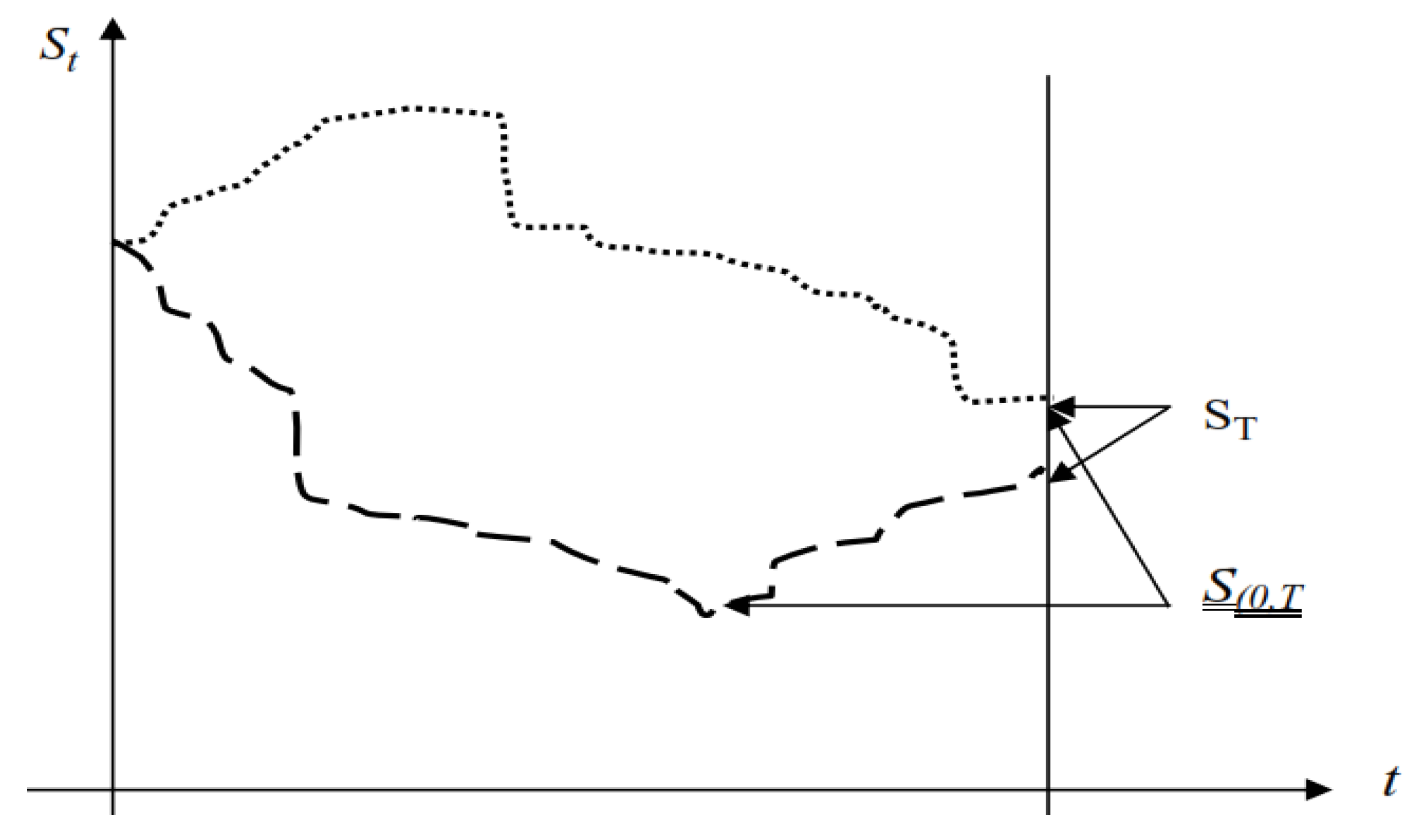
To understand the difference between T-day VaR and T-day MaxVaR at a confidence level α, let us look at Figure 1.

For the sake of simplicity, let us assume that the stock over a period of T days only traverses the two paths as shown in the diagram below. The stock price at any time t is given by S_t. S_T is the stock price at the end of the risk horizon and S_(0,T] is the minimum price that the stock hits across the path that it traverses. Mathematically, S_(0,T] = min {S_t, where t lies between (0, T]} In one of the paths, the minima occurs at the end of T days whereas, in the other, the minimum stock price can be observed at some point before the Tth day. The T-day VaR ignores the fact that a minima was reached before the Tth day, although the stock recovered towards the end of the holding period. It is concerned with the distribution of S_T, whereas MaxVaR takes this into account and depends on the distribution of S_(0,T].

Example 1.

Let the total/cumulative return on a portfolio at the end of T days be given by the following function

R = −400D − 225L + 100U

where D, L and U represent three different states of the world, and are mutually exclusive and collectively exhaustive. For the sake of simplicity, let us assume that all these states of the world are equally likely. This basically means that the chances of the portfolio losing USD 400 or losing USD 225 or gaining USD 100 is equal. Let us further assume that α = 5%. Thus, with a confidence level of 95% and by using the definition of VaR, VaR_α = USD 400.

Now, consider that the cumulative minimum return on the portfolio on or before T days is given by the following function

R_min = −675D − 225L − 111U

Again, assuming α = 5% and applying the definition of VaR on the minimum return function, we have VaR_α = USD 675. This is nothing but the MaxVaR. In other words, MaxVaR can also be defined as the VaR of the minimum return function over the risk horizon. Here, the MaxVaR of the portfolio is about 70% higher than the VaR.

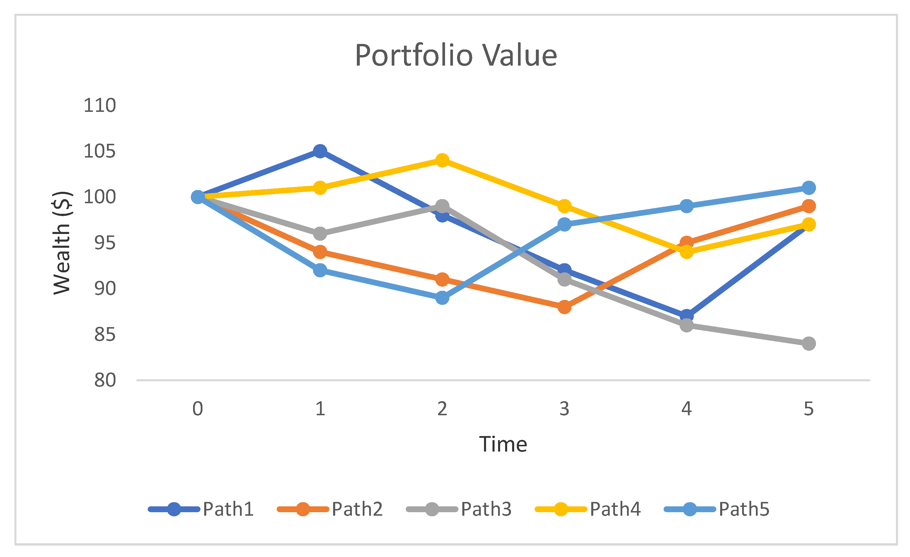
Example 2.

Let us consider a portfolio, the value of which is USD 100 at time t = 0. We are interested in finding out the probability that the portfolio would lose 10% of its value over a period of 5 days. For simplicity, we assume that there are five possible paths that the portfolio can traverse as shown in Figure 2. If we answer the question using a 5-day VaR, then the answer is 20%. From the figure, it is clear that only Path 3 ends up at a value less than USD 90 at the end of 5th day. However, the power of MaxVaR is evident from this example, as we can see that, except for Path 4, the portfolio breaches the barrier of USD 90 in every other path, which means that the probability that the portfolio would lose 10% of its value over a period of 5 days is 80%. With the help of this simple example, it is clear that the difference between MaxVaR and VaR can be large and substantial.

Note: The figure traces five possible paths for a portfolio over a 5-day period. The current value of the portfolio is USD 100. All possible paths (except Path 4) touches a wealth level of USD 90 over the 5-day period, whereas, at the end of the 5th day, only Path 3 has a value of USD 90 or less.

2.2. Properties of MaxVaR

Some of the important properties of MaxVaR and the inflation ratio as observed by Boudoukh et al. (2004) are as follows:

• MaxVaR decreases, with an increase in the drift or expected return given that other parameters are held constant. However, the ratio of MaxVaR to VaR increases as the drift affects the terminal returns more than the interim returns;
• With an increase in the risk horizon, the MaxVaR increases as expected. This also holds true for the inflation ratio;
• With other parameters kept constant, MaxVaR increases with an increase in volatility, but the MaxVaR to VaR ratio decreases;
• There is a decrease in the MaxVaR to VaR ratio at higher confidence levels;
• Discrete MaxVaR is lower than the continuous MaxVaR. This is obvious, as one can miss the minima when moving from a continuous framework to the discrete framework.

These properties were outlined by Boudoukh et al. (2004), assuming the normal distribution and constant volatility of the return series. They did show analytically1 how to derive MaxVaR from VaR and studied these properties for the Gaussian distribution. While using time-varying mean and volatility equations to model the returns with fat-tailed properties (P&L in this case), it might be analytically intractable to get a closed form expression to compute the MaxVaR; and hence, for simplicity purposes, one resorts to Monte Carlo simulation to empirically estimate the MaxVaR. We examine these properties as outlined above for fat-tailed P&L series of the options with time-varying volatility.

2.3. Model Specification

The P&L of the options can be approximated by the following equation2

$$P\&L\approx \delta R+\frac{1}{2}\gamma R^2$$

(1)

where R is the returns of the underlying stock and δ and γ are the option Greeks. Once we have the P&L of the options (as obtained from Equation (1)), we go ahead and fit a time-varying conditional volatility model to it. This is because we find that the series is auto-correlated and stationary (based on standard tests such as ADF and KPSS and time-series plots such as Acf and Pacf). To capture the heteroscedasticity and non-normality of the series, we fit an ARMA(1,1)-GARCH(1,1) model (time varying mean and volatility model) to the P&L of the options. The model so chosen is based on likelihood ratios such as Akaike Information Criteria (AIC) and Bayesian Information Criteria (BIC) and is shown below. Researchers (Bhattacharyya et al. 2008) do assume that the future returns of an asset are governed by the asset’s past returns and use different time series models for this purpose. For modelling purposes, let us denote the P&L of the options by $r_t$.

Model3:

$$r_t={\varphi }_0+{\varphi }_1{r}_{t-1}+{\theta }_1{\epsilon }_{t-1}+{\epsilon }_t$$

(2)

$${\epsilon }_t|\left({\epsilon }_{t-1},{\epsilon }_{t-2},{\epsilon }_{t-3}\dots ..{\epsilon }_1\right)~D\left(parameters\right)$$

(3)

$$h_t={\alpha }_0+{\alpha }_1{\epsilon }_{t-1}^2+{\beta }_1{h}_{t-1}$$

(4)

The usual restrictions apply on the parameters, i.e., $\left|{\varphi }_1\right|$ < 1; ${\alpha }_0,{\alpha }_1,{\beta }_1>0; {\alpha }_1+{\beta }_1<1$. Here, D denotes the distribution of the errors/innovations and $h_t$ denotes volatility at time t. We employ Pearson’s Type IV, Skewed Student’s t and Johnson’s SU distribution. These distributions can capture the skewness and high excess kurtosis, as observed in the P&L series, and have proven to be immensely successful in modelling similar empirical distributions. Some of the references can be found in Hu and Kercheval (2006, 2010), Bhattacharyya et al. (2008), Stavroyiannis et al. (2012), Zhu and Galbraith (2010). More details on these distributions, including their pdfs and parameter restrictions, can be found in Willink (2008), Zhu and Galbraith (2010) and Bhattacharyya and R (2012), among others.

2.4. Model Testing

In order to test the validity of the model, we use the standard back testing method by Kupiec (1995). Observed violations are defined as the number of instances the VaR/MaxVaR threshold is breached by the P&L of the Options for a given significance level α. Expected violations are the number of instances the VaR/MaxVaR threshold is expected to be breached and is calculated as the number of datapoints/days multiplied by the significance level α. The observed and expected violations are compared to check if the difference is statistically significant.

3. Data and Empirical Results

For the purpose of our study, we use the S&P 500 and FTSE 100 index options. In order to determine the volatility of the index options, we use the VIX and VFTSE indices for the corresponding period. The data4 (consisting of S&P 500, FTSE 100, VIX and VFTSE) are from January 2002 to November 2016 (approximately 3100 points). The source of the data is the Bloomberg terminal. The sample is divided into two parts in an 80:20 proportion, with the first part being used for model development and the second part used as a hold-out sample to validate the model predictions. We consider options with 30-day, 60-day and 90-day maturities. We estimate the MaxVaR and VaR at 1%, 2.5% and 5% significance levels and for a 10-day and 15-day risk horizon. The 10-day risk horizon is chosen based on the Basel norms and 15-day risk horizon for comparative purposes. Iqbal (2018) evaluated the expected shortfall estimates for European Options for a 1-day and 10-day risk horizon. Appropriate strike prices for the calls and a risk-free rate of 4% were also assumed for the entire duration. To summarise, the characteristics of the option under consideration are as follows:

Type: European Call	Risk-free rate: 4%
Maturity: 30 days/60 days/90 days	Position: Long
Moneyness: Out of money (K/S > 1)	Underlying5: FTSE 100/S&P 500

It is important to note that the risk-free rate has been taken as a constant for the purpose of simplicity and varying it with time does not change the insights presented in the paper. We conduct the study for six options (various combinations of the underlying and time to maturity of the option) and then conduct a sensitivity analysis by varying the moneyness of the option. We also compare the inflation factor for the option with that of the underlying stock.

Using the data, we estimate the P&L of the options using Equation (1). Then, we fit the time-varying mean and variance model, as described in Section 3, to the P&L of the options. This gives us the estimates of various parameters used in the model (maximum likelihood estimation technique (please see Bhattacharyya and R 2012) is used for the same). Once we have obtained the estimates of the parameters, our next step is to calculate the T-day VaR and MaxVaR using the Monte-Carlo simulation approach. This can be done using the following steps:

• We generate t random deviates. These random deviates are assumed to be the values for the innovations of the next t days. The distributions used to generate these innovations are Johnson’s SU, Pearson’s Type-IV and skewed Student’s t distribution. The parameters for these distributions are obtained by the maximum likelihood estimation procedure, as discussed earlier;
• Then, based on these random innovations generated in the previous step and by using the recursive mean and variance equations (2 and 4), we estimate the P&L for the next t days;
• The lowest cumulative value, as well as the T-day cumulative value of the P&L along the path (i.e., during the period of t days), is recorded;
• We repeat the above-mentioned steps N times (N = 25,000 in this case). The 25,000 values so recorded are sorted in an ascending order. The p% MaxVaR can then be calculated as the pth percentile of the empirical distribution (series with lowest cumulative values). We compare it with the T-day p% VaR, which is also calculated as the pth percentile of the empirical distribution (but from the series with the cumulative value for the entire T-day period);
• This process (i.e., all the steps mentioned above) is repeated for each and every datapoint in the training sample, i.e., we calculate the T-day VaR and MaxVaR for every datapoint in the sample and report the average value of the ratio;
• Once we determine the estimates of T-day VaR and MaxVaR, we then use standard back testing technique (Kupiec’s test) to check how good these estimates are.

Table 1. Summary statistics for the P&L of the index options.

	S&P 500 Index Option			FTSE 100 Index Option
	30-day	60-day	90-day	30-day	60-day	90-day
Mean	0.519	0.395	0.328	2.677	1.871	1.500
Median	0.267	0.331	0.365	0.656	0.721	0.758
Std. Dev	4.531	5.577	6.154	27.98	30.55	32.07
Maximum	54.77	56.65	57.59	296.6	281.6	276.4
Minimum	−9.854	−19.81	−28.11	−70.01	−114.9	−139.5
Skewness	1.988	1.076	0.706	1.578	0.926	0.653
Excess Kurtosis	14.486	8.206	6.666	10.074	6.562	5.568

Note: The table shows the descriptive statistics for the P&L of the index options. In general, the skewness is positive and the distribution is heavy tailed. The observed skewness and kurtosis are statistically significant and different from zero with p-values of the order of 10⁻⁵.

gives us the summary statistics of the P&L of the index options. From the figures in the table, it is clearly evident that the P&L series is heavy-tailed and skewed. This reinforces the argument that normal distribution cannot be used to approximate such a series. These characteristics of the P&L series indicate that the probability of a heavy loss is higher than that given by the normal distribution. The probability of getting large negative returns is different from the probability of getting large positive returns.

4. Observation and Discussion

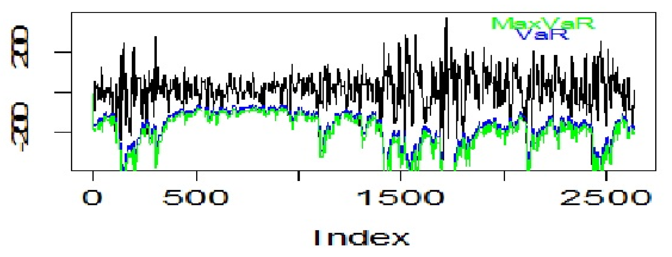
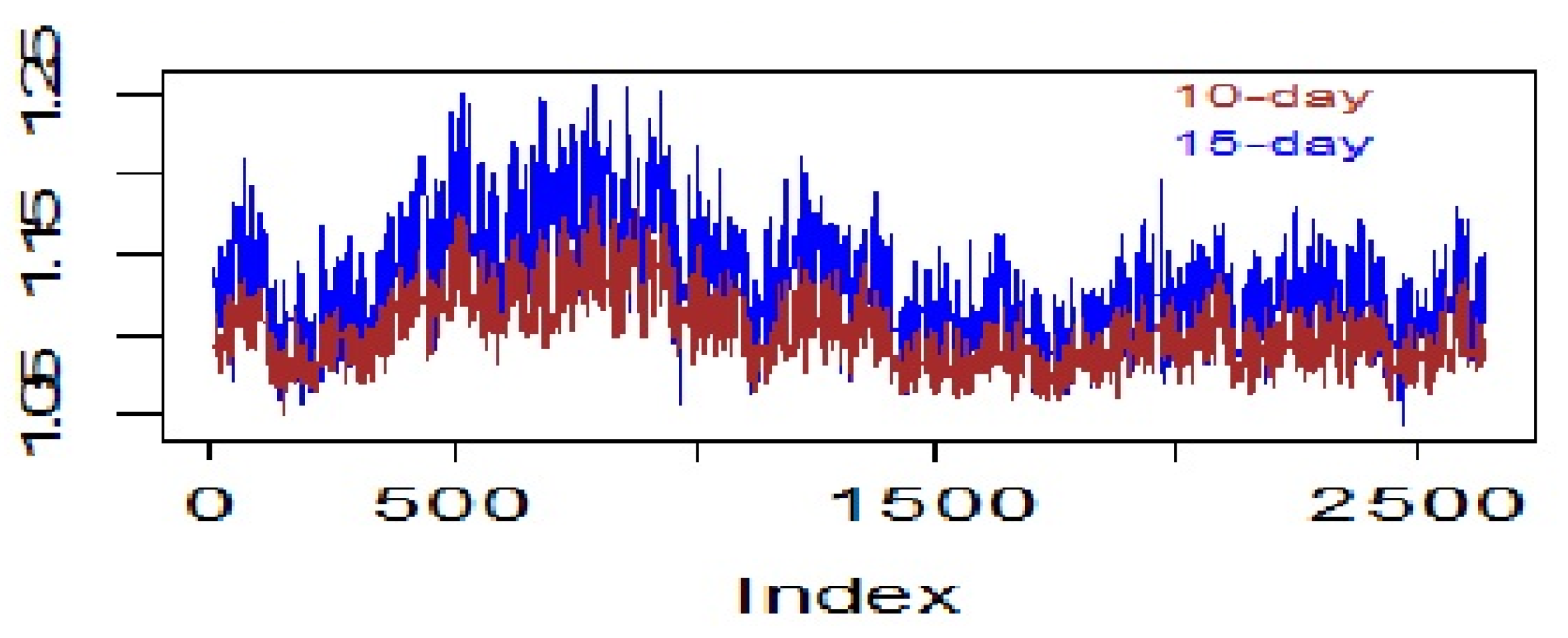
Figure 3 depicts the difference between the 15-day VaR and MaxVaR for a 60-day maturity FTSE 100 index option at 2.5% significance level. Figure 4, which shows the variation in MaxVaR to VaR ratio for all the datapoints of the P&L of the 30-day maturity FTSE 100 index option, reinforces this finding, as we can see that the 10-day ratio is consistently below the 15-day ratio.

The numbers in

Table 2. Back-testing results for 10-day VaR.

Observed Violations	S&P 500 Index Option			FTSE 100 Index Option			Expected Violations
	30-day	60-day	90-day	30-day	60-day	90-day
Pearson IV
1%	5 **	16	18	17	23	24	26
2.5%	67	67	67	71	70	70	65
5%	146	143	149	156	153	152	130
Johnson’s SU
1%	0 **	16	17	16	22	24	26
2.5%	60	59	60	67	65	65	65
5%	144	134	134	154	147	142	130
Skewed Student’s t
1%	0 **	15	16	8 **	17	23	26
2.5%	52	57	62	61	65	67	65
5%	136	134	134	149	148	148	130

Note: The table shows us number of observed and expected violations for 10-day VaR assuming different distributions on the errors in the P&L of the options. The numbers marked with ** indicate that the difference between expected and observed violations is significant at 1% level.

,

Table 3. Back-testing results for 10-day MaxVaR.

Observed Violations	S&P 500 Index Option			FTSE 100 Index Option			Expected Violations
	30-day	60-day	90-day	30-day	60-day	90-day
Pearson IV
1%	29	29	28	23	24	24	26
2.5%	76	69	70	71	67	66	65
5%	161 **	158	150	147	155	159	130
Johnson’s SU
1%	31	31	32	18	18	19	26
2.5%	68	69	66	67	71	81 **	65
5%	124	126	129	132	138	139	130
Skewed Student’s t
1%	18	18	19	21	20	20	26
2.5%	66	67	66	71	71	72	65
5%	111	141	119	144	146	116	130

Note: The table gives us the no. of observed and expected violations for 10-day MaxVaR assuming different distributions on the errors in the P&L of the options. The numbers marked with ** indicate that the difference between expected and observed violations is significant at 1% level.

,

Table 4. Back-testing results for 15-day VaR.

Observed Violations	S&P 500 Index Option			FTSE 100 Index Option			Expected Violations
	30-day	60-day	90-day	30-day	60-day	90-day
Pearson IV
1%	25	20	18	33	25	21	26
2.5%	63	49	47 **	75	60	58	65
5%	157	118	109	141	121	108	130
Johnson’s SU
1%	22	19	16	16	29	19	26
2.5%	58	61	56	62	59	67	65
5%	128	122	143	136	128	131	130
Skewed Student’s t
1%	11 **	17	34	18	18	19	26
2.5%	60	62	62	59	63	64	65
5%	119	120	147	141	134	138	130

Note: The table shows us the no. of observed and expected violations for 15-day VaR assuming different distributions on the errors in the P&L of the options. Numbers marked with ** indicate that the difference between expected and observed violations is significant at 1% level.

and

Table 5. Back-testing results for 15-day MaxVaR.

Observed Violations	S&P 500 Index Option			FTSE 100 Index Option			Expected Violations
	30-day	60-day	90-day	30-day	60-day	90-day
Pearson IV
1%	23	20	19	30	27	25	26
2.5%	57	56	51	87 *	70	67	65
5%	109	116	110	134	117	113	130
Johnson’s SU
1%	21	19	19	32	29	23	26
2.5%	58	55	53	77	68	66	65
5%	111	119	117	131	123	118	130
Skewed Student’s t
1%	29	16	18	21	23	22	26
2.5%	58	62	66	67	66	68	65
5%	110	116	146	124	142	116	130

Note: The figures give the no. of observed and expected violations for 15-day MaxVaR assuming different distributions in the errors on the P&L of the options. Numbers marked with * indicate that the difference between expected and observed violations is significant at 1% level.

give us the observed and expected violations for 10-day and 15-day VaR and MaxVaR for FTSE 100 and S&P 500 index options with different maturities at various significance levels. The standard back testing method by Kupeic is used to examine whether the difference in the expected and observed violations is statistically significant at 1% level. In most of the instances, we find that this is not the case and the expected and observed violations are statistically not different, hence validating the model used to predict T-day (10 and 15) VaR and MaxVaR. This means that any of the heavy-tailed and skewed distributions among Johnson’ SU distribution, Pearson’s Type IV distribution and skewed Student’s t distribution can be used to model the residuals/innovations of the P&L of the options. We also observe that, at 1% significance level, Pearson’s Type IV distribution outperforms the other two, as the difference between the expected and observed violations is the least when it is assumed that residuals follow Pearson’s Type IV distribution. The same can be said about Johnson’s SU distribution at 5% significance level.

The figures in

Table 6. Average 10-day Inflation factor.

10-day MaxVaR to VaR Ratio	S&P 500 Index Option			FTSE 100 Index Option
	30-day	60-day	90-day	30-day	60-day	90-day
Pearson IV
1%	1.142	1.123	1.116	1.086	1.077	1.073
2.5%	1.207	1.173	1.160	1.133	1.115	1.108
5%	1.308	1.245	1.222	1.203	1.169	1.158
Johnson’s SU
1%	1.146	1.129	1.118	1.088	1.075	1.071
2.5%	1.211	1.178	1.165	1.136	1.114	1.109
5%	1.311	1.239	1.226	1.192	1.167	1.161
Skewed Student’s t
1%	1.147	1.119	1.114	1.089	1.079	1.074
2.5%	1.214	1.177	1.162	1.134	1.117	1.111
5%	1.306	1.248	1.219	1.201	1.171	1.159

Note: The figures in the table give the average 10-day MavVaR to VaR ratio for the P&L of the S&P 500 and FTSE 100 index options with different time to maturities and varying distributional assumptions on the residuals.

and

Table 7. Average 15-day Inflation factor.

15-day MaxVaR to VaR Ratio	S&P 500 Index Option			FTSE 100 Index Option
	30-day	60-day	90-day	30-day	60-day	90-day
Pearson IV
1%	1.183	1.152	1.139	1.113	1.097	1.091
2.5%	1.271	1.211	1.191	1.171	1.142	1.132
5%	1.413	1.302	1.266	1.260	1.207	1.189
Johnson’s SU
1%	1.176	1.149	1.141	1.116	1.099	1.089
2.5%	1.269	1.201	1.187	1.177	1.139	1.131
5%	1.397	1.311	1.274	1.268	1.211	1.191
Skewed Student’s t
1%	1.179	1.151	1.138	1.118	1.102	1.096
2.5%	1.277	1.216	1.193	1.169	1.141	1.134
5%	1.404	1.309	1.278	1.257	1.206	1.192

Note: The table shows average 15-day MavVaR to VaR ratio for the P&L of the S&P 500 and FTSE 100 index options with different time to maturities and varying distributional assumptions on the residuals.

suggest that MaxVaR, on average, is about 11% higher than VaR and it increases to about 30% for S&P 500 index option at a higher significance level of 5% for a 10-day risk horizon. For FTSE 100 index options, the range is between 7% and 20%. For a 15-day risk horizon, this ratio increases for both FTSE 100 and S&P 500 index options at all significance levels, irrespective of the distributional assumptions on the residuals. However, for an FTSE 100 index option, the ratio now varies from 1.09–1.26; in the case of the S&P 500 index option, it varies from 1.14–1.41. This is because of the fact that, although both MaxVaR and VaR increase with an increase in the risk-horizon, the increase in MaxVaR is steeper than that of VaR. The results are in agreement with those observed by Kritzman and Rich (2002), wherein the authors argued that the time diversification property does not hold for MaxVar, unlike VaR.

This basically means that unlike VaR, which decreases with time for a long enough risk horizon (say 5 years or so), MaxVaR always increases with an increase in the risk horizon.

We also observe that the MaxVaR to VaR ratio increases with an increase in significance levels which agree with the findings from an earlier work in the area (refer to Section 2 on the properties of MaxVaR). This finding is true for options with different maturities and for both S&P 500 and FTSE 100 index options. We also find that the ratio increases with a decrease in the time to maturity of the option at a given significance level. The trend holds true for both the index options. The reason for this could be attributed to the fact that options with lower maturities are more influenced by speculations as compared to options which have a longer time to maturity. This can also be concluded from the summary statistics of the P&L of the index options as the mean return of the P&L is higher for options with lower time to maturity and we know from the earlier literature (refer to Section 2 on properties of MaxVaR) that the MaxVaR to VaR ratio is directly proportional to the mean return and inversely proportional to the volatility/variance. We also study and compare the inflation factor of the P&L of the options with that of the underlying stock returns. The results are summarised in

Table 8. Summary statistics for the 10-day Inflation factor.

10-day MaxVaR to VaR Ratio	S&P 500 Index		FTSE 100 Index
	Stock	Option	Stock	Option
Average
1%	1.137	1.115	1.085	1.072
2.5%	1.213	1.178	1.113	1.098
5%	1.362	1.299	1.152	1.131
Maximum
1%	1.174	1.167	1.121	1.119
2.5%	1.268	1.256	1.147	1.141
5%	1.514	1.466	1.190	1.182
Minimum
1%	1.095	1.066	1.051	1.029
2.5%	1.160	1.107	1.084	1.057
5%	1.254	1.180	1.119	1.084

Note: The table shows average, maximum and minimum 10-day MavVaR to VaR ratios for the S&P 500 and FTSE 100 index returns and for the P&L of the corresponding 30-day index options at various significance levels.

and

Table 9. Summary statistics for the 15-day inflation factor.

15-day MaxVaR to VaR Ratio	S&P 500 Index		FTSE 100 Index
	Stock	Option	Stock	Option
Average
1%	1.156	1.131	1.100	1.086
2.5%	1.239	1.200	1.131	1.114
5%	1.403	1.332	1.173	1.151
Maximum
1%	1.203	1.192	1.139	1.138
2.5%	1.299	1.295	1.170	1.169
5%	1.545	1.526	1.217	1.211
Minimum
1%	1.119	1.072	1.058	1.042
2.5%	1.177	1.118	1.094	1.071
5%	1.281	1.185	1.126	1.096

Note: The table gives us average, maximum and minimum 15-day MavVaR to VaR ratios for the S&P 500 and FTSE 100 index returns and for the P&L of the corresponding 30-day index options at various significance levels.

.

While Table 8 presents a comparative view of the 10-day MaxVaR to VaR ratio of the P&L of both the index options and the underlying returns at various significance levels, Table 9 presents the 15-day inflation factor. From the figures, it is interesting to note that, on average, the inflation factor is higher for stocks than for the options, which is unexpected as options have a non-linear pay off structure and interim risk exposure for them is expected to be higher than the underlying stocks.

While it is indeed true that the MaxVaR for options is higher than that of the underlying stock, but when compared to end-of-horizon risk, i.e., T-day VaR, the increase in MaxVaR is less than the increase in VaR (for the options vis-à-vis the stock), thereby decreasing the overall ratio or the inflation factor. Although the pattern observed in the P&L of the options and for the underlying stock returns over a period of t days is similar, the level of increase/drop (when compared to the previous day) is different. The change is higher for the stock returns than the P&L of the options. This is the reason for the difference in MaxVaR to VaR ratio between the P&L and the underlying stock returns. Further, as explained in Section 2 above, we know that the MaxVaR to VaR ratio or the inflation factor is directly related to the mean and inversely related with the volatility (for more details, please refer to Boudoukh et al. (2004)). From the data we find that, while the mean of the P&L of options is greater than that of the average returns of the underlying, the P&L of the options are highly volatile as well. The high volatility effect dominates the high mean effect, and as a result the inflation factor for the options decreases when compared to the underlying stock indices. A closed form expression for the adjustment factor under the normality assumption for returns is proposed by Boudoukh et al. (2004). The empirical findings in this study indicate that, although the exact closed form expression may no longer hold when the normality assumption is relaxed, the broad relationships with the various parameters are still preserved6.

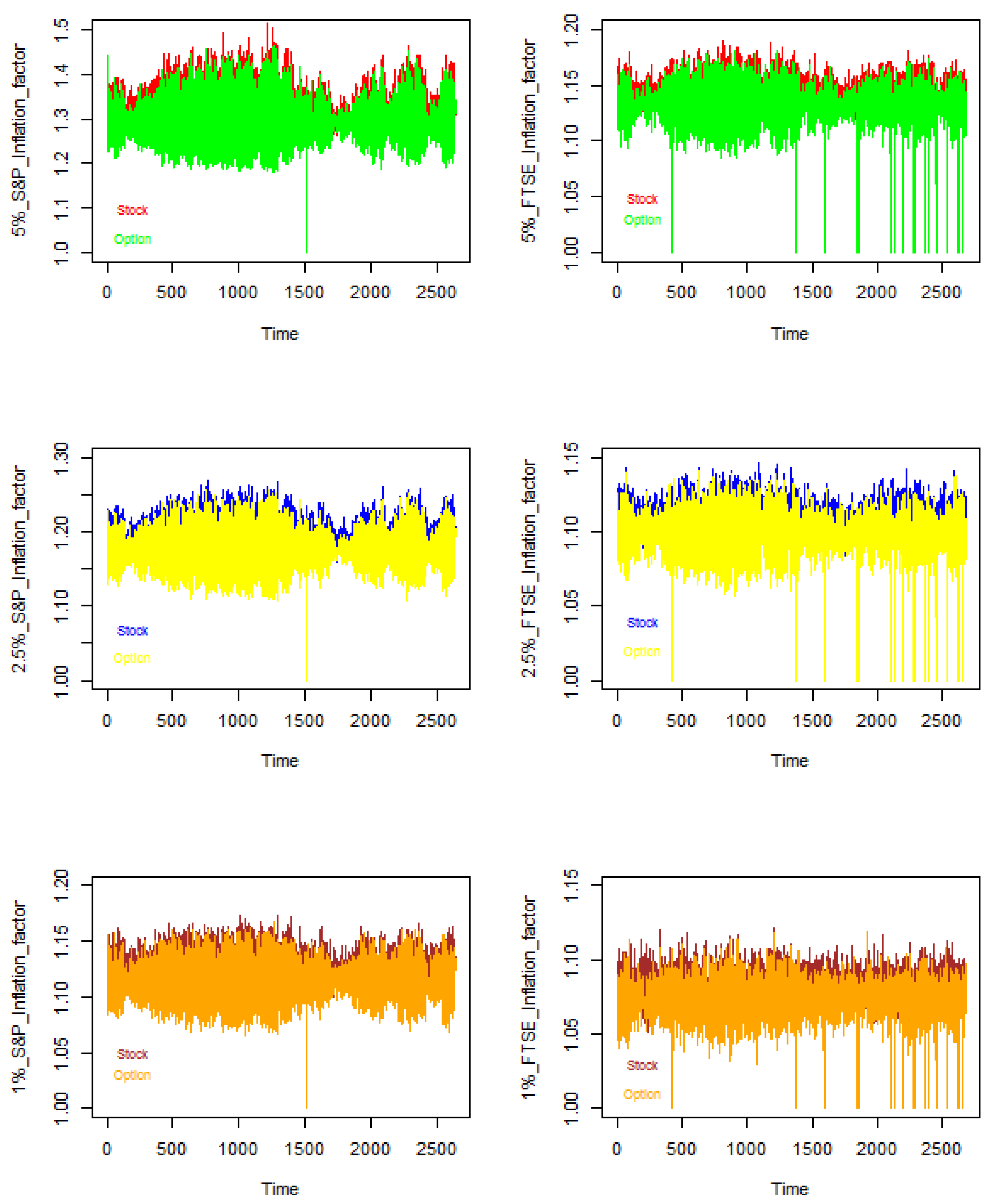
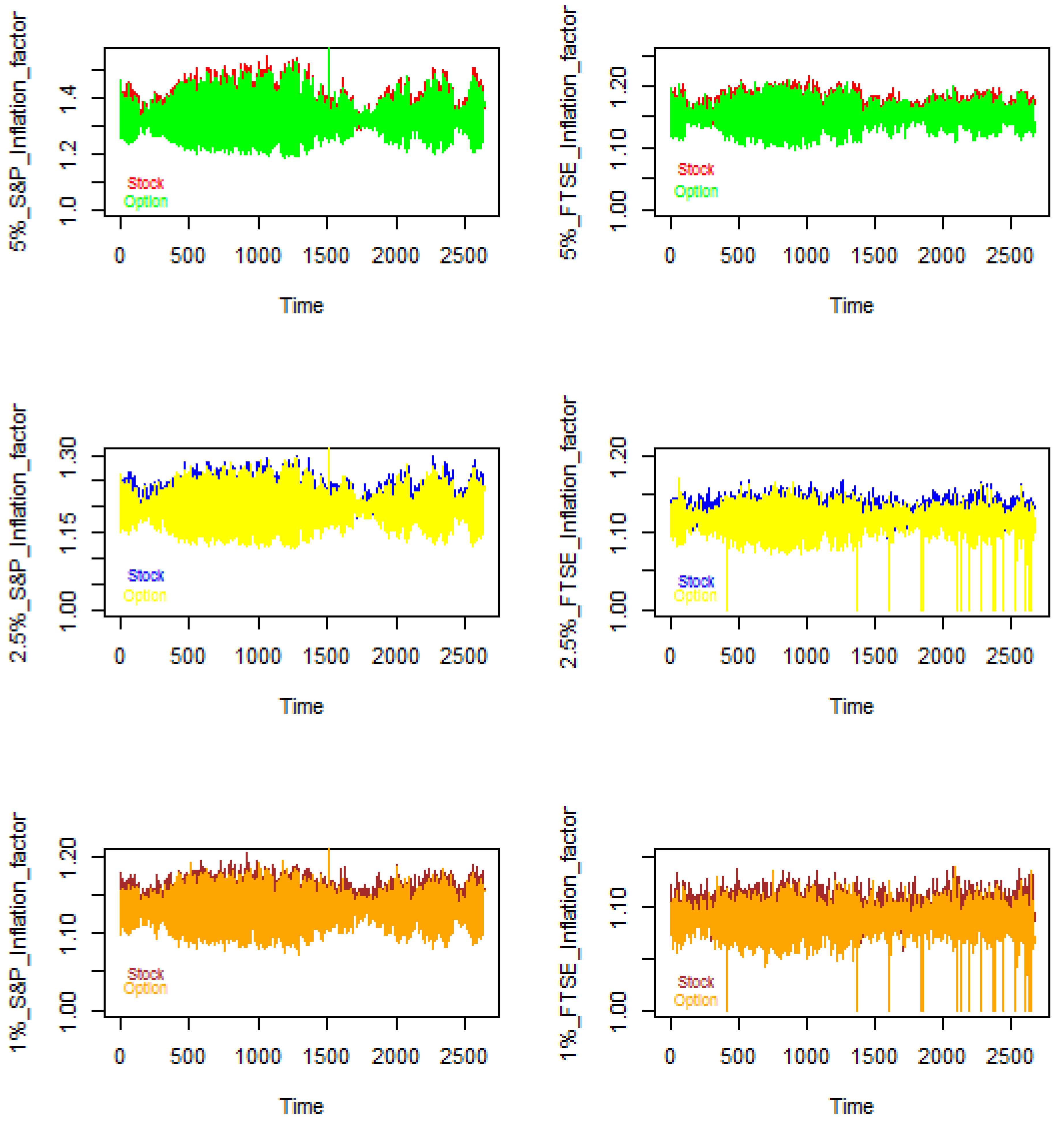
Figure 5 and Figure 6 show us how the MaxVaR to VaR ratio for a 30-day index option varies with that of the underlying stock at various significance levels for the period under study. While Figure 5 is a depiction of the 10-day inflation factor, Figure 6 illustrates the 15-day inflation factor. We find that in most cases (about 80% for FTSE 100 and 72% for S&P 500 index), the inflation factor for the underlying stock exceeds that of the index option.

Table 10. Variation in 15-day Inflation factor with respect to moneyness of the option.

15-day MaxVaR to VaR Ratio	S&P 500 Index Option			FTSE 100 Index Option
	30-day	60-day	90-day	30-day	60-day	90-day
K/S = 0.95
1%	1.117	1.116	1.114	1.083	1.082	1.081
2.5%	1.156	1.156	1.154	1.118	1.117	1.116
5%	1.213	1.211	1.207	1.167	1.165	1.163
K/S = 1
1%	1.156	1.137	1.128	1.106	1.094	1.089
2.5%	1.218	1.187	1.174	1.157	1.136	1.128
5%	1.311	1.259	1.239	1.233	1.196	1.183
K/S = 1.05
1%	1.208	1.161	1.145	1.149	1.112	1.099
2.5%	1.316	1.228	1.200	1.242	1.166	1.145
5%	1.506	1.329	1.279	1.412	1.248	1.211

Note: The figures in the table show average 15-day MavVaR to VaR ratio for the P&L of the S&P 500 and FTSE 100 index options with different time to maturities and varying degree of moneyness. Innovations/residuals of the P&L of the options follow Pearson’s Type IV distribution.

gives us the 15-day MaxVaR to VaR ratio for the P&L of the S&P 500 and FTSE 100 index options with varying time to maturities at various significance levels. The moneyness of the option is varied from 0.9–1.1 and three instances are reported (K/S = 0.95/1/1.05). Here, we assume that the innovations/residuals of the P&L of the options follow Pearson’s Type IV distribution. We find that the average inflation factor varies from 1.15 to 1.41. It is also observed that, with an increase in moneyness of an option, the average inflation factor increases.

As observed, we find that MaxVaR as a risk measure for options is vastly different from VaR. From the numbers reported, we can say that VaR gives us a more conservative risk estimate as it reports the risk of the portfolio only at the end of the time horizon, whereas the potential risk that the portfolio is exposed to is given by MaxVaR and the difference between them could be as large as 40%, as seen in Table 6.

Hence, as a risk measure, MaxVaR gives us more information as compared to VaR and, since the difference between them could be very high, MaxVaR may prove to be a more useful measure of risk in the context of options. This is true from both the retail investor’s as well as the regulator’s perspective.

5. Practical Implications

The models presented in this paper to estimate the interim risk exposure for a portfolio of options can be used in practice by traders, investors and regulators. They can help the traders in the efficient construction and management of portfolios containing options. In case of an investor, these models give her a better idea about the risk involved over the entire holding period of the portfolio and hence, she can make an informed decision about investing in a portfolio of options, keeping in view the prospective margin calls. Even for a regulator, these models could help in monitoring the risk exposure of various institutions who have invested in portfolios which include options.

Further, policy announcements by the Central Bank and its impact on the portfolio rebalancing by the institutional investors could present an additional challenge for the regulator. If we look at VaR (end of the horizon) as a risk measure, the risk exposure for the institutional investors might not get impacted, but the interim risk exposure is definitely prone to changes as MaxVaR measures the risk during the risk horizon and not only at the end.

6. Conclusions

In this paper, our objective was to test the performance of MaxVaR as an alternative risk measure for a portfolio of options. We also wanted to test the sensitivity of MaxVaR with respect to the time to maturity of the option. We also study the variation in the inflation factor (i.e., MaxVaR to VaR ratio) with the significance levels, the risk horizon and the moneyness of the option, and conduct a comparative analysis vis-à-vis the inflation factor of the underlying stock index. We find that MaxVaR as an alternative risk measure could be a significant improvement from the existing risk measure of VaR in the context of options. We observe that MaxVaR can exceed VaR by a huge margin (as high as 41%). We also find that the difference between MaxVaR and VaR varies with the risk horizon and increases with an increase in the risk horizon. This is because of the inherent properties of MaxVaR asnd VaR. While MaxVaR increases monotonically with an increase in the risk horizon, VaR increases at a lower rate with an increase in risk horizon and later decreases. With respect to the significance levels, we find that the MaxVaR to VaR ratio decreases with a decrease in the significance level, i.e., as we move more and more towards the tail of the P&L distribution, we find that the difference in MaxVaR and VaR reduces. We also find that with an increase in moneyness of the option (for the range under study), the inflation factor increases at all significance levels and time to maturities. The analysis has been carried out with the residuals of the P&L being assumed to follow different heavy-tailed and skewed distributions.

In comparison to the underlying stock, the inflation factor of the index option is observed to be lower at all significance levels under study. This is because of the difference in the inherent characteristics of the P&L of the option and the returns of the underlying stock index. These findings can be significant in our endeavor to understand the options and the risk associated with them. Using MaxVaR as a risk measure, one can carefully plan his/her investments, and with a greater understanding of the risk involved, he/she can manage the portfolio even better. There is still further scope for research in the area. The study can be extended to a complex portfolio of path dependent options and one can study the sensitivity of the results with respect to other parameters that affect the price of an option.