Estimating Stochastic Volatility under the Assumption of Stochastic Volatility of Volatility


Abstract
:1. Introduction
2. Model Specification
3. Estimation Technique
4. Application
5. Financial Implications
6. Conclusions
Author Contributions
Funding
Conflicts of Interest
References
- Alghalith, Moawia. 2012. New methods of estimating volatility and returns: Revisited. Journal of Asset Management 13: 307–9. [Google Scholar] [CrossRef]
- Alghalith, Moawia. 2016. Estimating the Stock/Portfolio Volatility and the Volatility of Volatility: A New Simple Method. Econometric Reviews 35: 257–62. [Google Scholar] [CrossRef]
- Amendola, Alessandra, Manuela Braione, Vincenzo Candila, and Giuseppe Storti. 2020. A Model Confidence Set approach to the combination of multivariate volatility forecasts. International Journal of Forecasting. [Google Scholar] [CrossRef]
- Andersen, Torben G., and Jesper Lund. 1997. Estimating continuous-time stochastic volatility models of the short-term interest rate. Journal of Econometrics 77: 343–77. [Google Scholar] [CrossRef]
- Asai, Manabu, and Michael McAleer. 2011. Alternative asymmetric stochastic volatility models. Econometric Reviews 30: 548–64. [Google Scholar] [CrossRef] [Green Version]
- Asai, Manabu, Michael McAleer, and Jun Yu. 2006. Multivariate stochastic volatility: A review. Econometric Reviews 25: 145–75. [Google Scholar] [CrossRef]
- Barndorff-Nielsen, Ole E., and Almut E. D. Veraart. 2013. Stochastic Volatility of Volatility and Variance Risk Premia. Journal of Financial Econometrics 11: 1–46. [Google Scholar] [CrossRef]
- Barndorff-Nielsen, Ole E., P. Reinhard Hansen, Asger Lunde, and Neil Shephard. 2009. Realized kernels in practice: Trades and quotes. The Econometrics Journal 12: C1–C32. [Google Scholar] [CrossRef]
- Bekaert, Geert, and Marie Hoerova. 2014. The VIX, the variance premium and stock market volatility. Journal of Econometrics 183: 181–92. [Google Scholar] [CrossRef]
- Boukhetala, Kamal. 1996. Modelling and Simulation of a Dispersion Pollutant with Attractive Center. Southampton: Computational Mechanics Publications, Boston: Computational Mechanics Inc. [Google Scholar]
- Caporin, Massimiliano, and Michael McAleer. 2012. Do We Really Need Both BEKK and DCC? A Tale of two Multivariate GARCH Models. Journal of Economic Surveys 26: 736–51. [Google Scholar] [CrossRef] [Green Version]
- Cohen, Jerome B., Fischer Black, and Myron Scholes. 1972. The valuation of option contracts and a test of market efficiency. Journal of Finance 27: 399–418. [Google Scholar] [CrossRef]
- Comte, Fabienne, Valentine Genon-Catalot, and Yves Rozenholc. 2010. Nonparametric estimation for a stochastic volatility model. Finance and Stochastics 14: 49–80. [Google Scholar] [CrossRef] [Green Version]
- Corsi, Fulvio, Stefan Mittnik, Christian Pigorsch, and Uta Pigorsch. 2008. The volatility of realized volatility. Econometric Reviews 27: 46–78. [Google Scholar] [CrossRef]
- Cox, John C., Jonathan E. Ingersoll Jr., and Stephen A. Ross. 1985. A Theory of the Term Structure of Interest Rates. Econometrica 53: 385. [Google Scholar] [CrossRef]
- Cui, Zhenyu, J. Lars Kirkby, and Duy Nguyen. 2017. A general framework for discretely sampled realized variance derivatives in stochastic volatility models with jumps. European Journal of Operational Research 262: 381–400. [Google Scholar] [CrossRef]
- Ghysels, Eric, Andrew C. Harvey, and Eric Renault. 1996. Stochastic volatility. In Handbook of Statistics. Edited by Maddala Gangadharrao. Amsterdam: North-Holland, vol. 14, pp. 119–91. [Google Scholar]
- Hansen, Peter Reinhard, and Zhuo Huang. 2016. Exponential GARCH Modeling With Realized Measures of Volatility. Journal of Business & Economic Statistics 34: 269–87. [Google Scholar] [CrossRef]
- Heston, Steven L. 1993. A Closed-Form Solution for Options with Stochastic Volatility with Applications to Bond and Currency Options. The Review of Financial Studies 6: 327–43. [Google Scholar] [CrossRef] [Green Version]
- Huang, Darien, Christian Schlag, Ivan Shaliastovich, and Julian Thimme. 2019. Volatility-of-volatility risk. Journal of Financial and Quantitative Analysis 54: 2423–52. [Google Scholar] [CrossRef] [Green Version]
- Hull, John, and Alan White. 1987. The pricing of options on assets with stochastic volatility. Journal of Finance 42: 281–300. [Google Scholar] [CrossRef]
- Liu, Lily Y., Andrew J. Patton, and Kevin Sheppard. 2015. Does anything beat 5-min RV? A comparison of realized measures across multiple asset classes. Journal of Econometrics 187: 293–311. [Google Scholar] [CrossRef] [Green Version]
- Maasoumi, Esfandiar, and Michael McAleer. 2008. Realized Volatility and Long Memory: An Overview. Econometric Reviews 27: 1–9. [Google Scholar] [CrossRef]
- Mandelbrot, Benoit. 1963. The variation of certain speculative prices. Journal of Business 36: 394–419. [Google Scholar] [CrossRef]
- Mrázek, Milan, Jan Pospíšil, and Tomáš Sobotka. 2016. On calibration of stochastic and fractional stochastic volatility models. European Journal of Operational Research 254: 1036–46. [Google Scholar] [CrossRef]
- Officer, Robert R. 1973. The variability of the market factor of the New York stock exchange. Journal of Business 46: 434–53. [Google Scholar] [CrossRef]
- Park, Yang-Ho. 2015. Volatility-of-volatility and tail risk hedging returns. Journal of Financial Markets 26: 38–63. [Google Scholar] [CrossRef]
- Poon, Ser-Huang, and Clive W. J. Granger. 2003. Forecasting Volatility in Financial Markets: A Review. Journal of Economic Literature 41: 478–539. [Google Scholar] [CrossRef]
- Renò, Roberto. 2006. Nonparametric estimation of stochastic volatility models. Economics Letters 90: 390–95. [Google Scholar] [CrossRef]
- Shephard, Neil. 2005. Stochastic Volatility: Selected Readings. Oxford: Oxford University Press. [Google Scholar]
- Vetter, Mathias. 2015. Estimation of integrated volatility of volatility with applications to goodness-of-fit testing. Bernoulli 21: 2393–418. [Google Scholar] [CrossRef] [Green Version]
- Wong, Hoi Ying, and Yu Wai Lo. 2009. Option pricing with mean reversion and stochastic volatility. European Journal of Operational Research 197: 179–87. [Google Scholar] [CrossRef]
| 1 | Stochastic volatility is an essential component in an asset pricing model, in option pricing. See (Wong and Lo 2009; Mrázek et al. 2016; Cui et al. 2017; among others). |
| 2 | Heston (1993) assumed that the variance follows a square root process, , where σ controls the volatility of volatility. When σ is equal to zero, the volatility is deterministic. Following Heston (1993) and applying Ito’s rule (4), we are able to test whether volatility is stochastic via linear regression equations. We refer to the study implemented by Heston (1993) for more information regarding this issue. |
| 3 | Following Barndorff-Nielsen et al. (2009), (1) we deleted the entries with a timestamp outside the 9:30 a.m.–4 p.m. window when the market is open and (2) we deleted the entries with a bid, ask or a transaction price equal to zero. |
| 4 | For the simulation analysis, we considered a stochastic process of a single random variable based on the S&P 500 index assuming that the variance varies over time (i.e., exhibits serial correlated properties). To this end, we used a stochastic differential equation of the Ito type. The drift and the diffusion parameters are estimated from the original series by the method of maximum pseudo-likelihood (see Boukhetala 1996). |
| 5 | Following Bekaert and Hoerova (2014), the squared index can be decomposed into the variance of equity returns and the variance risk premium. For robustness purposes, in order to isolate the predictive power of past volatility and the volatility on volatility risk premium, we estimated (15) and (16) using the difference between the VIX indices and daily realized variance (estimated as the sum of 5-min intraday returns of the S&P 500) as dependent variables. In this regard, we also used in (15) and (16) the residuals obtained from and their squared specifications as dependent variables. In all cases, the results remain qualitative and quantitatively similar. |


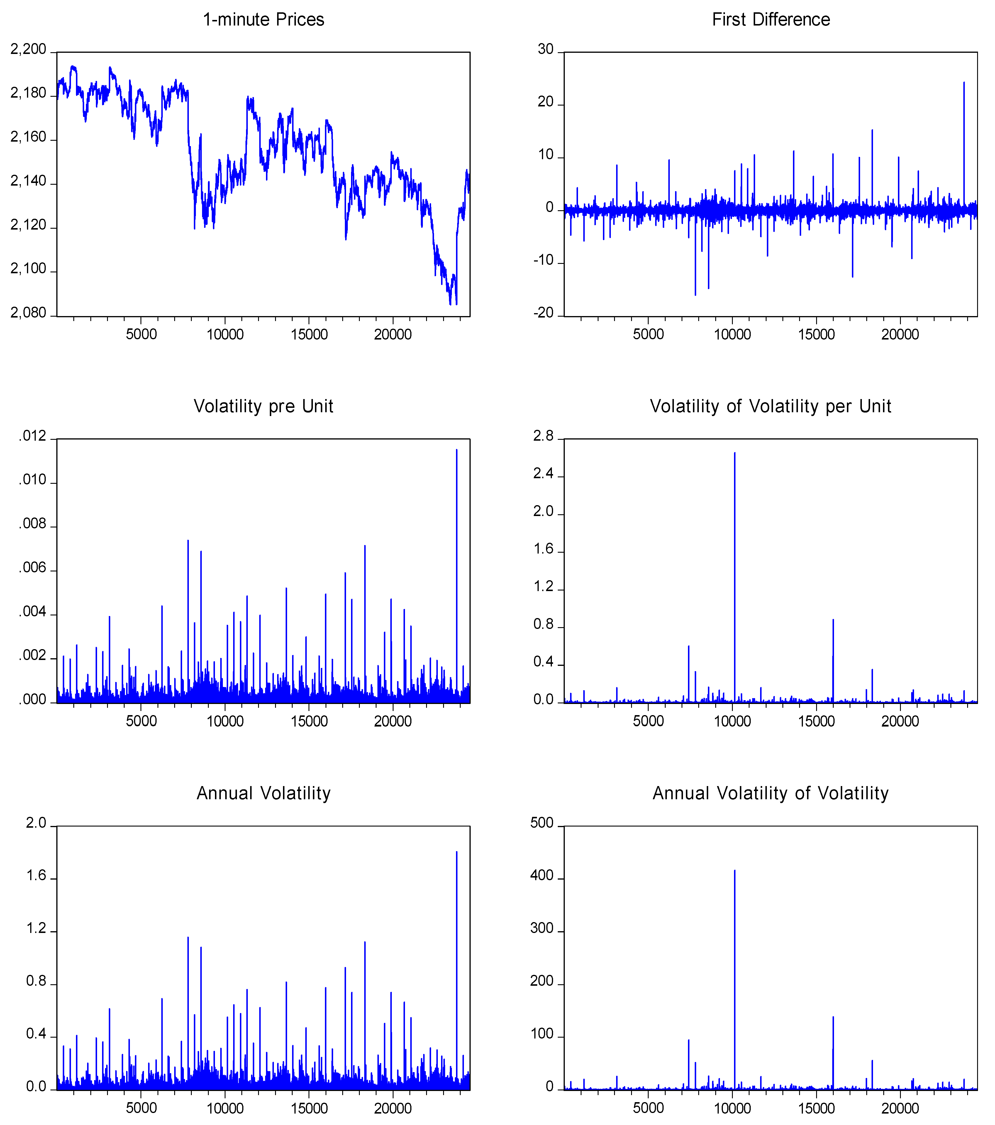
| Panel A: 1-Min Sample | ||||
| vt | γt | vt (annual) | γt (annual) | |
| Mean | 1.59E-04 | 1.05E-03 | 2.4883E-02 | 1.65E-01 |
| Median | 1.03E-04 | 1.73E-04 | 1.6142E-02 | 2.71E-02 |
| Maximum | 1.15E-02 | 2.66E+00 | 1.8062E+00 | 4.16E+02 |
| Minimum | 0.00E+00 | 4.16E-11 | 0.0000E+00 | 6.52E-09 |
| Std. Dev. | 2.32E-04 | 1.91E-02 | 3.6384E-02 | 3.00E+00 |
| Skewness | 1.37E+01 | 1.16E+02 | 1.3678E+01 | 1.16E+02 |
| Kurtosis | 4.21E+02 | 1.55E+04 | 4.2115E+02 | 1.55E+04 |
| Jarque–Bera | 1.80E+08 | 2.43E+11 | 1.8000E+08 | 2.43E+11 |
| p-value | [0.00E+00] | [0.00E+00] | [0.00E+00] | [0.00E+00] |
| No. of obs. | 24,224 | 24,224 | 24,224 | 24,224 |
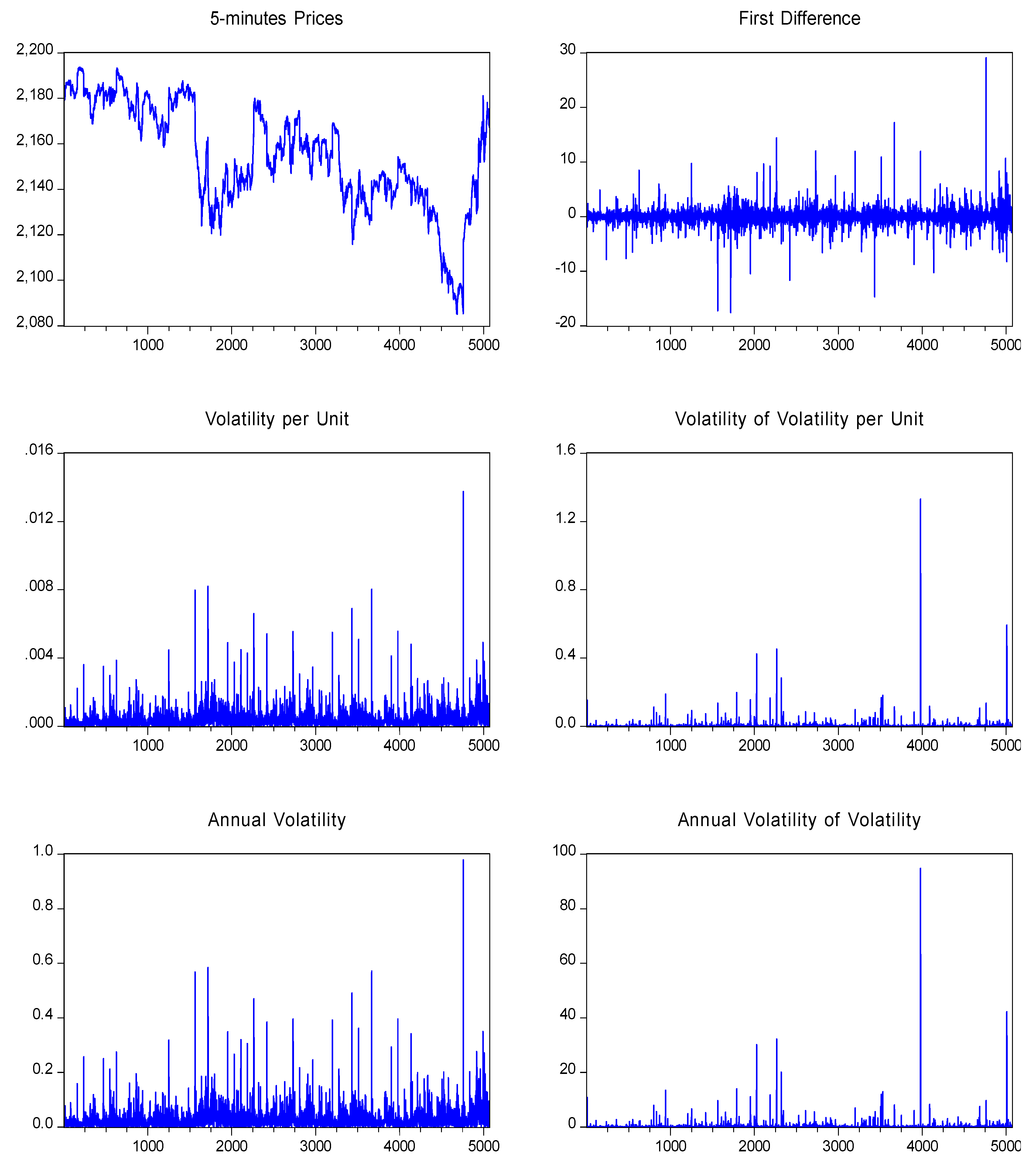
| Panel B: 5-Min Sample | ||||
| vt | γt | vt (annual) | γt (annual) | |
| Mean | 4.16E-04 | 2.96E-03 | 2.96E-02 | 2.11E-01 |
| Median | 2.66E-04 | 4.43E-04 | 1.89E-02 | 3.15E-02 |
| Maximum | 1.37E-02 | 1.33E+00 | 9.79E-01 | 9.48E+01 |
| Minimum | 4.56E-06 | 1.06E-09 | 3.25E-04 | 7.52E-08 |
| Std. Dev. | 5.67E-04 | 2.47E-02 | 4.04E-02 | 1.76E+00 |
| Skewness | 6.98E+00 | 3.69E+01 | 6.98E+00 | 3.69E+01 |
| Kurtosis | 1.02E+02 | 1.78E+03 | 1.02E+02 | 1.78E+03 |
| Jarque–Bera | 2.08E+06 | 6.63E+08 | 2.08E+06 | 6.63E+08 |
| Probability | [0.00E+00] | [0.00E+00] | [0.00E+00] | [0.00E+00] |
| p-value | 5042 | 5042 | 5042 | 5042 |
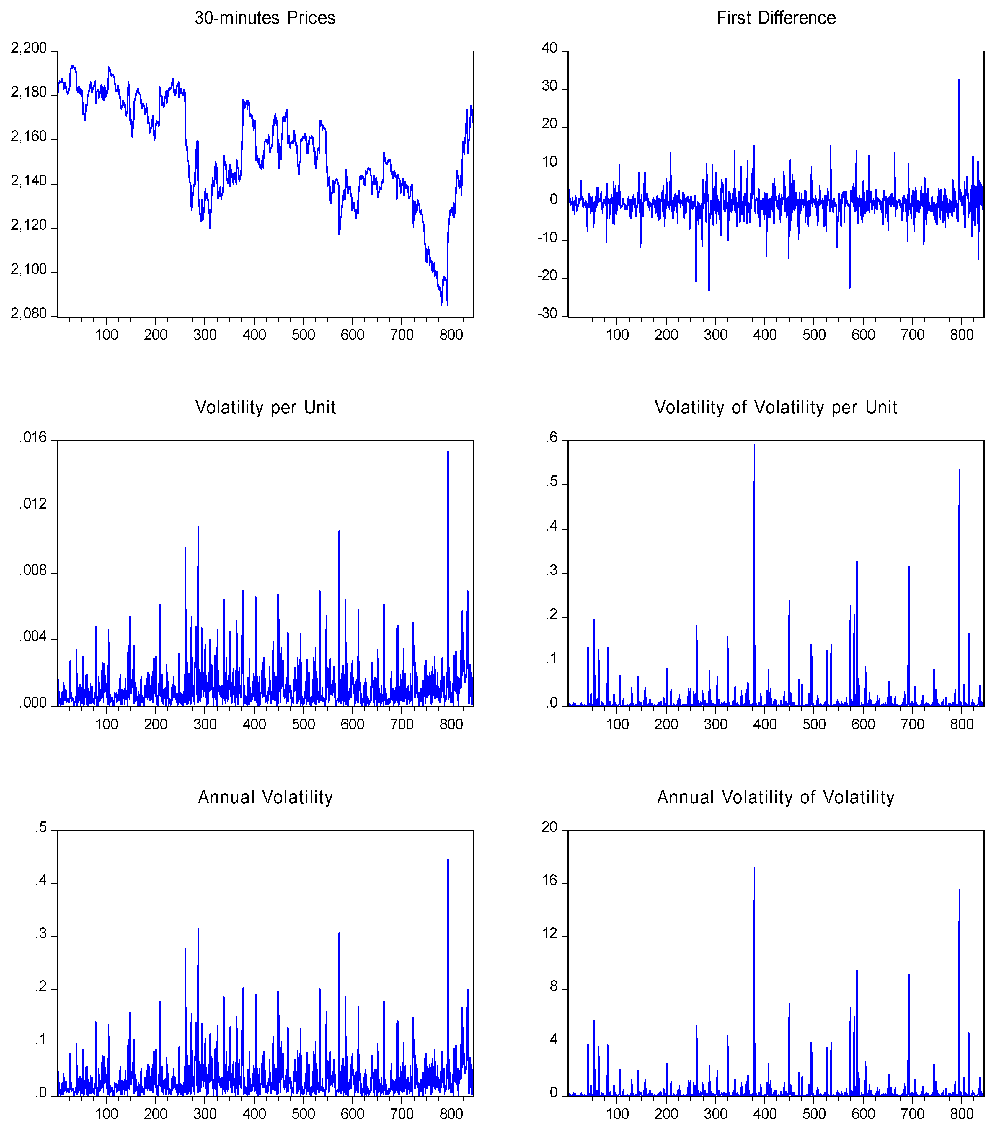
| Panel C: 30-Min Sample | ||||
| vt | γt | vt (annual) | γt (annual) | |
| Mean | 1.14E-03 | 3.31E-02 | 9.56E-03 | 2.78E-01 |
| Median | 7.18E-04 | 2.09E-02 | 1.32E-03 | 3.83E-02 |
| Maximum | 1.53E-02 | 4.46E-01 | 5.91E-01 | 1.72E+01 |
| Minimum | 4.66E-06 | 1.35E-04 | 2.49E-07 | 7.25E-06 |
| Std. Dev. | 1.38E-03 | 4.02E-02 | 3.90E-02 | 1.13E+00 |
| Skewness | 3.63E+00 | 3.63E+00 | 9.34E+00 | 9.34E+00 |
| Kurtosis | 2.48E+01 | 2.48E+01 | 1.13E+02 | 1.13E+02 |
| Jarque–Bera | 1.84E+04 | 1.84E+04 | 4.38E+05 | 4.38E+05 |
| p-value | [0.00E+00] | [0.00E+00] | [0.00E+00] | [0.00E+00] |
| No. of obs. | 841 | 841 | 841 | 841 |
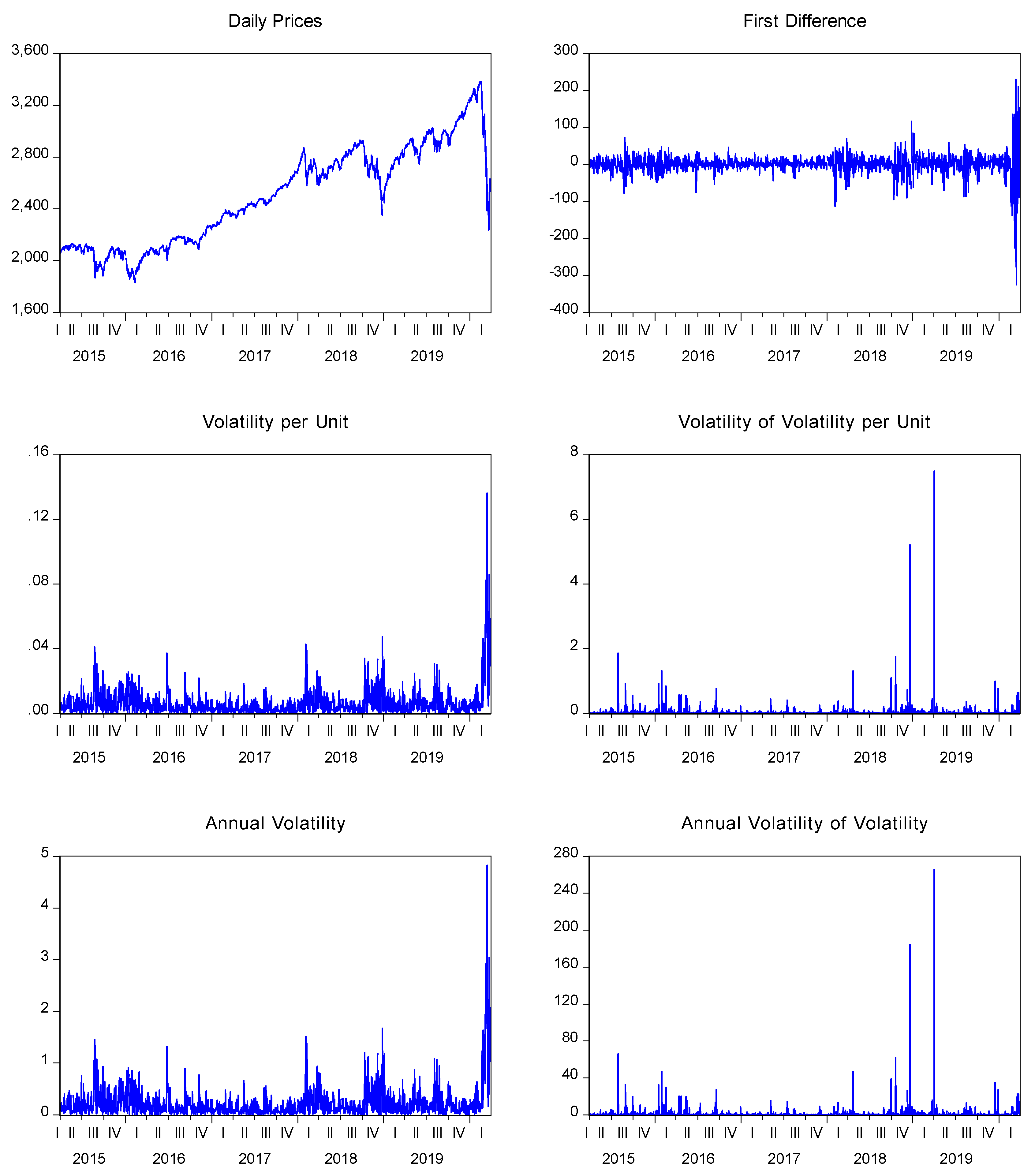
| Panel D: Daily Sample | ||||
| vt | γt | vt (annual) | γt (annual) | |
| Mean | 6.60E-03 | 4.84E-02 | 2.34E-01 | 1.71E+00 |
| Median | 3.77E-03 | 7.28E-03 | 1.33E-01 | 2.58E-01 |
| Maximum | 1.36E-01 | 7.49E+00 | 4.83E+00 | 2.66E+02 |
| Minimum | 6.87E-06 | 3.20E-05 | 2.43E-04 | 1.13E-03 |
| Std. Dev. | 9.54E-03 | 2.87E-01 | 3.38E-01 | 1.02E+01 |
| Skewness | 5.45E+00 | 1.93E+01 | 5.45E+00 | 1.93E+01 |
| Kurtosis | 5.18E+01 | 4.48E+02 | 5.18E+01 | 4.48E+02 |
| Jarque-Bera | 1.31E+05 | 1.04E+07 | 1.31E+05 | 1.04E+07 |
| p-value | [0.00E+00] | [0.00E+00] | [0.00E+00] | [0.00E+00] |
| No. of obs. | 1256 | 1256 | 1256 | 1256 |
| Panel A: 1-Min Sample | |||||
| Case 1: Returns | Case 2: Simulation | ||||
| 8.82E-05 *** | 0.3892 | 8.49E-05 | 0.3789 | ||
| (7.05E-07) | (7.15E-07) | ||||
| Panel B: 5-Min Sample | |||||
| Case 1: Returns | Case 2: Simulation | ||||
| 1.23E-04 *** | 0.3779 | 1.16E-04 | 0.3688 | ||
| (2.22E-06) | (2.28E-06) | ||||
| Panel C: 30-Min Sample | |||||
| Case 1: Returns | Case 2: Simulation | ||||
| 1.36E-04 *** | 0.341 | 1.76E-05 | 0.3184 | ||
| (6.40E-06) | (5.46E-06) | ||||
| Panel D: Daily Sample | |||||
| Case 1: Returns | Case 1: Returns | ||||
| 6.54E-03 *** | 0.3677 | 3.21-E04 | 0.3810 | ||
| (2.40E-04) | (1.37E-05) | ||||
| Panel A: 1-Min Sample | |||||
| Case 1: Returns | Case 2: Simulation | ||||
| 6.95E+00 *** | 0.4937 | 6.25E+00 | 0.4889 | ||
| (4.56E-02) | (6.01E-02) | ||||
| Panel B: 5-Min Sample | |||||
| Case 1: Returns | Case 2: Simulation | ||||
| 1.68Ε+00 *** | 0.4770 | 1.22E+00 | 0.4462 | ||
| (2.48E-02) | (1.85E-02) | ||||
| Panel C: 30-Min Sample | |||||
| Case 1: Returns | Case 2: Simulation | ||||
| 2.87E-01 *** | 0.4491 | 3.16E-01 | 0.4214 | ||
| (1.09E-02) | (2.40E-02) | ||||
| Panel D: Daily Sample | |||||
| Case 1: Returns | Case 2: Simulation | ||||
| 5.02E+01 *** | 0.4710 | 7.99E+01 | 0.3914 | ||
| (1.50E+00) | (1.20E-01) | ||||
| Panel A: Units | |||
| VIX Index | |||
| Wald test | |||
| 4.23E+02 *** | 1.33E+01 *** | 0.2381 | 46.2936 |
| (8.86E+00) | (2.94E-01) | [0.00E+00] | |
| VVIX Index | |||
| Wald test | |||
| 7.60E+02 *** | 7.63E+00 *** | 0.1175 | 25.6088 |
| 2.94E+01 | 9.76E-01 | [0.00E+00] | |
| Panel B: Logarithm Units | |||
| VIX Index | |||
| Wald test | |||
| 2.50E+01 *** | 6.19E-01 *** | 0.2953 | 39.8077 |
| (6.47E-01) | (2.05E-02) | [0.00E+00] | |
| VVIX Index | |||
| Wald test | |||
| 7.73E+00 *** | 8.16E-02 *** | 0.1414 | 23.9296 |
| (8.16E-02) | (1.06E-02) | [0.00E+00] | |
© 2020 by the authors. Licensee MDPI, Basel, Switzerland. This article is an open access article distributed under the terms and conditions of the Creative Commons Attribution (CC BY) license (http://creativecommons.org/licenses/by/4.0/).
Share and Cite
Alghalith, M.; Floros, C.; Gkillas, K. Estimating Stochastic Volatility under the Assumption of Stochastic Volatility of Volatility. Risks 2020, 8, 35. https://doi.org/10.3390/risks8020035
Alghalith M, Floros C, Gkillas K. Estimating Stochastic Volatility under the Assumption of Stochastic Volatility of Volatility. Risks. 2020; 8(2):35. https://doi.org/10.3390/risks8020035
Chicago/Turabian StyleAlghalith, Moawia, Christos Floros, and Konstantinos Gkillas. 2020. "Estimating Stochastic Volatility under the Assumption of Stochastic Volatility of Volatility" Risks 8, no. 2: 35. https://doi.org/10.3390/risks8020035