The Leaders, the Laggers, and the “Vulnerables”

Abstract

We examine the lead-lag effect between the large and the small capitalization financial institutions by constructing two global weekly rebalanced indices. We focus on the 10% of stocks that “survived” all the rebalancings by remaining constituents of the indices. We sort them according to their systemic importance using the marginal expected shortfall (MES), which measures the individual institutions’ vulnerability over the market, the network based MES, which captures the vulnerability of the risks generated by institutions’ interrelations, and the Bayesian network based MES, which takes into account different network structures among institutions’ interrelations. We also check if the lead-lag effect holds in terms of systemic risk implying systemic risk transmission from the large to the small capitalization, concluding a mixed behavior compared to the index returns. Additionally, we find that all the systemic risk indicators increase their magnitude during the financial crisis.

1. Introduction

Seeking for positive expected return and managing portfolio risk are two sides of the same coin, accompanied by a risk-return trade-off that depends on the risk appetite of the market participants. The early literature includes many studies that focus on the behavior of asset returns and the possibility of significant profits due to information diffusion. One of the major financial economic concerns is to understand how firms transmit information to markets and how markets impose this information on stock prices. Traditional asset-pricing theories assume that information is disseminated instantaneously in a complete and frictionless market. However, there is a considerable empirical reason to believe that investors are facing significant frictions, and information can sometimes be slowly transmitted to the market. Specifically, there is ample evidence pointing to a lead-lag effect on equity markets where the stock prices of some firms show a delayed reaction to other firms’ price innovations. Lo and MacKinlay (1990) mentioned that the forecasting ability of stock returns can be attributed to what is known as the “stock market overreaction” hypothesis, based on the waves of optimism or pessimism of investors creating a “momentum”. Hou (2007) primarily focused on explaining the lead-lag effect as a sluggish reaction of certain firms to common information compared to others. The author conditioned on the industry membership, because slow diffusion of common information should be more prevalent among firms from the same industry, and he showed that within the same industry, large firms lead small firms. DeMiguel et al. (2014) studied whether investors can exploit serial dependence in stock returns to improve out-of-sample portfolio performance. Using raw returns rather than returns in excess of the risk-free rate and a rolling-horizon procedure, they estimated a VAR model of a small and large stock portfolio and verified a lead-lag relationship with large stock returns leading small stock returns.

In this study, we also restricted to a single industry, that is financial institutions. Why financial institutions? The fact that a healthy financial system is the backbone of economic progress is addressed by many papers1. Additionally, the waves of optimism or pessimism are not limited to one institution as the financial system’s structure is comprised of many financial institutions with linkages between them that may transfer and magnify financial stress during times of crisis (e.g., Billio et al. 2012). The financial institutions’ connectivity is investigated in many works focusing on the systemic risk2, emphasizing the importance of the financial system’s structure during systemic events and the homogeneity or asset commonality between financial institutions3. The works in Wagner (2010) and Allen et al. (2012) pointed out that an increasing homogeneity between financial institutions makes them vulnerable to the same risks, as they become more similar to each other. The former Fed Chairman, Paul Volcker, supported imposing restrictions on the risk level of large banks, on their size, their interconnections, and activities (Volcker 2012).

The systemic risk as a function of the financial system’s architecture and the size of the financial institutional participants is still under debate among regulators and researchers, especially that large banks were found to have an integral role at the center of the recent financial crisis; see Laeven et al. (2016). The authors studied the significant variation in the cross-section of systemic risk measures of large banks during the recent financial crisis in a broad sample of countries, intending to identify bank-specific factors, like banks size, capital, funding, and activities, that determine systemic risk and shed light on the ongoing debate on the merits of restricting bank size, imposing capital surcharges on large banks, and/or restricting their unstable funding and risky activities. Several theories support the view that large and complex banks contribute to systemic risk. According to one view, which the authors named “the unstable banking hypothesis”, large banks tend to engage in risky activities more (e.g., trading) and to be financed more by short-term debt, which makes them more vulnerable to generalized liquidity shocks and market failures such as liquidity shortages and fire sales (Kashyap et al. 2002; Shleifer and Vishny 2010; Gennaioli et al. 2013). In our view, the importance and the implications of this “hypothesis” are not addressed much by the literature. We chose to expand the sample of financial institutions to a broader one because the results of a shock and its dissemination have not been studied or highlighted so far. For example, the removal of the floor of the Euro/Swiss franc exchange rate from the Swiss National Bank was at a time when the markets were not turbulent. However, some financial services companies have been insolvent due to poorly, for such an event, margined positions. The questions that arise are: How much can the insolvency of small financial institutions become a problem? Who are the “vulnerable” portfolio constituents? Can a financial institution be vulnerable, but at the same time a leader in terms of returns?

The literature discussing measures of banks’ systemic risk is vast, and Benoit et al. (2017) provided an excellent survey of systemic risk measures. The literature either uses only market data, i.e, financial returns or credit default swaps (CDS) (e.g., Billio et al. 2012; Acharya et al. 2012; Allen et al. 2012; Adrian and Brunnermeier 2016), or enriches the dataset with balance sheet data (among others, Brownlees and Engle (2017)) to measure systemic risk. A combination of both microeconomic and macroeconomic data was used by Calabrese and Giudici (2015), who built a statistical model of bank distress, based on the balance sheet of a bank, and on macroeconomic information on the country where the bank operated. Several authors discussed the systemic risk vulnerability in the context of financial networks facing the challenge to provide not only a good fit, but also a good interpretation. This may result in choosing a model that has little support from the data, leading to predictions worse than could be obtained with other models. Additionally, the graphical models are essentially static, photographing a situation in a given period. This assumption seems to be restrictive in economics, in the case of variables that change over time, for example during periods of financial stress. Giudici and Green (1999) and recently in Ahelegbey et al. (2016) proposed more advanced, Bayesian, graphical models to overcome this limitation. Battiston et al. (2012) contributed to the debate on the resilience of financial networks by introducing a dynamic model for the evolution of financial robustness, showing that, in the presence of financial acceleration and persistence, the probability of default did not decrease monotonically with diversification. As a result, the financial network was most resilient for an intermediate level of connectivity. Diebold and Yilmaz (2014) proposed several connectedness measures built from pieces of variance decompositions, and they argued that they provided natural and insightful measures of connectedness. They also showed that variance decompositions define weighted, directed networks, so that our connectedness measures are intimately related to key measures of connectedness used in the network literature. Building on these insights, they tracked daily time-varying connectedness of major U.S. financial institutions’ stock return volatilities in recent years, with emphasis on the financial crisis of 2007–2008. Abedifar et al. (2017) compared the results of three different measures to gauge systemic risk, employing an application of the graphical network model described by Giudici and Spelta (2016) to identify the most interconnected banking sector. Avdjiev et al. (2019), based on a tensor decomposition method that extracted an adjacency matrix from a multi-layer network, proposed a distress measure for national banking systems that incorporated not only banks’ CDS spreads, but also how they interacted with the rest of the global financial system via multiple linkage types, using banks’ foreign exposures. Despite the vast amount of literature, there is no widely accepted methodology to determine the systemically important nodes in a network. To answer this, Battiston et al. (2012) introduced the DebtRank metric to determine the impact of the distress of one or several financial institutions through their counterparties’ network. Soramaki and Cook (2013) introduced SinkRank to predict the influence of disturbance caused by the collapse of a bank and identify most affected banks in the system, and Brunnermeier and Cheridito (2019) developed SystRiskto capture the a priori cost to society for providing tail-risk insurance to the financial system. In addition, Elliott et al. (2014) proposed a simple model of cross-holdings to analyze cascades in financial networks; they concluded that diversification and integration of financial institutions had non-monotonic effects on financial contagions, whereas Amini et al. (2016) considered the magnitude of contagion in large counterparty network, giving analytical expression for the asymptotic fraction of defaults, emphasizing in this way the key role of contagious links via the institutions with large connectivity and a large fraction of contagious links.

To measure systemic risk, we used the marginal expected shortfall (MES) of Acharya et al. (2017) and its alternatives proposed by Hashem and Giudici (2016). MES is simply calculated by each firm’s average return during the C% worst days for the market. It measures how exposed a firm is to the aggregate tail shocks, and together with leverage, it has a significant explanatory power for which firms contribute to a potential crisis (see, Acharya et al. 2017). Additionally and for the portfolio allocation, we used MES because, under the assumption that the individual financial institution and the index returns are driven by a bivariate GARCH, the MES of the financial institution is proportional to its systematic risk, as measured by its time-varying beta (see Benoit et al. 2017). On the other hand, there is much criticism of the systemic risk measures, and various papers have presented their shortcomings (among others, Danielsson et al. 2016; Benoit et al. 2019; Idier et al. 2014). The discussion of the adequacy of the systemic risk measures is out of the scope of this paper, and we chose to use MES and its two alternatives, for three main reasons: First, the stock returns used for its calculation are easily obtained and updated, contrary to the balance sheet data used in other measures that are updated at a quarterly frequency. Second, MES provides a clear measure of the expected loss of financial institutions when an extreme event occurs. Third is its additive property. The sum of MES from all banks is equal to a measure of the total systemic risk, allowing for macroprudential tools to be implemented at the bank level (see Tarashev et al. 2010; Qin and Zhou 2013). The disadvantage of this method is that it does not reflect characteristics like the size and the leverage. However, we would like to address that MES is based on historical data like measures of risks built on the covariance matrix. Given the uniqueness of each crisis, the assumption that the risk measures or the parameters involved in their calculation are sufficiently invariant makes these measures “forensic” tools, as Malevergne and Sornette (2006) pointed out. Therefore, MES complements other forensic approaches without being a forward-looking indicator for an upcoming crisis.

This paper contributes to the size and interconnectedness debates in three ways:

• First, we examine the lead-lag effect reported by Lo and MacKinlay (1990) between large and small capitalization financial index returns. To obtain the two indexes, we divide the financial institutions based on their market capitalization into top ones that are the largest until reaching the top 50th percentile of market capitalization and the remaining bottom ones, repeating this procedure on a weekly basis over the pre- and post-financial crisis period of 2007. We choose to use market capitalization (market cap), as it is widely used to create a context for judging company financial performance and business outlook. Larger cap tend to have more broadly diversified business structures than smaller firms. This may give them more stable business performance from year-to-year, with relatively less variable earnings and revenue streams. As a result, large companies may have less volatile share prices than smaller firms in many circumstances. Large companies generally have also tended to be the least sensitive to economic headwinds. Smaller companies, on the other hand, tend to have a tighter business focus. They may have the potential for more rapid revenue and profit growth, but this potential is often more variable. As a result, small-company shares may be, on average, more volatile and more sensitive to macroeconomic shifts than the shares of larger companies.
• Second, we form a large and a small cap portfolio of the stocks that remained as index constituents in every rebalance (named “survived” large and small cap stocks), and we test whether the lead-lag effect is sustained within the systemic risk measures of those. For this purpose, we use a non-directional systemic risk measure, which does not take size into account upon its construction. This allows us to control for the contemporaneous size effect that results from the systemic risk measure specification. Thus, we use the bivariate marginal expected shortfall (MES) systemic risk measure of Acharya et al. (2017) to estimate the risk exposure of an individual institution to the market.
• Third, we test if the size impact holds upon taking into consideration the financial system structure. The use of network analysis gives insightful information about important players in terms of network connectivity. For this purpose, we use two alternatives of MES that take the interconnectedness relations into account: the network based MES (NetMES), which extends MES by taking multivariate dependencies into its estimation; and the Bayesian NetMES, which further accounts for the network model uncertainty.

We further investigate the size impact at the individual institution level. Upon the estimation of MES, NetMES, and Bayesian NetMES, we rank the institutions based on the systemic risk indicators in descending order for the systemic risk level. We select the top six ranking institutions across the different systemic risk measures, and we evaluate their network connectedness.

The paper is organized as follows: Section 2 describes in detail the dataset and the construction of the large and the small capitalization indices. Section 3 states the VAR model, which explains the lead-lag relation between the large and the small cap index returns and tests its statistical significance to identify the origin of the predictability in index returns. Section 4 discusses the systemic risk indicators, and Section 5 presents the results of the lead-lag relations between the systemic risk indicators. We also give details about the systemically important financial institutions derived from the previous analysis. Section 6 concludes.

2. Data and Market Indices

We examined the interrelations between the large and small capitalization financial stocks by constructing our own indices, instead of using an existing benchmark market index. An already available index would be like a black box, as details like the constituents of the index, the weights in each distinct point of time, and the re-balancing dates are unknown. Indeed, comparing the available benchmark market indices, three separate causative influences can be uncovered. First, the behavior of equity indices is partly attributable to the technical procedures of its construction. Some indices have a small number of stocks, while others have a large number4. Some local benchmark market indices are industrially concentrated, while others are very diversified. These diversification elements explain part of the observed inter-market differences in price indices’ behavior, which do not correspond to differences in the individual stocks behaviors. Second, local indices may vary in their industrial composition and have industries that are inherently more or less volatile. We can think of a local index as a country-specific managed portfolio with particular industry sector “bets”. In this context, even a large portfolio can be influenced by disproportionate investments in certain industries. Third, exchange rates play a significant role. With returns expressed in a local currency, part of a stock index’s return volatility is induced by monetary phenomena such as changes in anticipated and actual local inflation rates. Converting local currency returns into common currency returns (e.g., the U.S. dollar) does not entirely eliminate the exchange rate’s influence.

The steps followed to construct our indices were: First, we collected stocks across the globe, which according to the Global Industry Classification Standard (GICS) were classified as banks and diversified financial institutions, excluding consumer finance, diversified financial services, insurance, and real estate companies. The fact that our sample contained a wide range of financial institutions and not only banks allowed us to take into account other sources of risks. In particular, our sample contained financial institutions exposed to sovereign systemic risk (the case of Greece during the debt crisis), to geographic risk (for example, periods of turmoil in Middle Eastern countries), and/or to risks driven by different banking business models (e.g., banks, asset management and custody banks, etc.). We remark that, as the GICS was applied to companies around the world and it was annually revised, the universe was continuously up-to-date and, therefore, so were our results. Second, we divided them into two tiers: the top 50 sequential percentile rank and the bottom 50 sequential percentile rank, obtaining the large and the small capitalization groups, respectively. The sample was free of survivorship, restatement, and lagging bias and contained the five largest world companies, which accounted for 63.02% of the 2010 world banking sector and represented the fundamentals as they were known in the market at each observation point. Then, all the stock prices were converted into U.S. dollars, since according to Roll (1992), the best way to combine stocks in the same industry, but traded in different currencies was to convert all first to a common currency and then construct the industry index. Beginning from 31 December 2014, and going back to 1 January 2005, our portfolio was weekly rebalanced, ending up with 522 different groups of large and small capitalization financial stocks. During the coverage period, the indices covered 2590 stocks; 1361 appeared in the weekly large cap portfolios and 2064 in the small cap portfolios, and 835 stocks moved between the two groups. The set of large cap stocks spanned 98 countries, 3 industry groups (Banks, Capital Markets, Thrifts & Mortgage), 6 sub-industries (Asset Management & Custody Banks, Diversified Banks, Diversified Capital Markets, Investment Banking & Brokerage, Regional Banks, Thrifts & Mortgage Finance)5, and 103 primary exchanges. For the small cap stocks group, there were 108 countries and 118 primary exchanges. The number of industry and sub-industry groups was the same. Only 321 out of 1361 large cap stocks “survived” through the years in each rebalance, having a positive weight in the indices. On the other hand, 193 out of the 2064 small cap stocks survived. In both cases, we called these groups as “survived”. Following the sub-industry classifications, from the 321 large cap survived financial institutions, 39 belonged to the Asset Management & Custody Banks (AMC), 131 to the Diversified Banks (DB), 8 to the Diversified Capital Markets (DCM), 19 to the Investment Banking & Brokerage (IBB), 98 to the Regional Banks (RB), and 11 to the Thrifts & Mortgage Finance (TMF) sub-industry. Accordingly, from the 193 small cap survived financial institutions, 23 belonged to the Asset Management & Custody Banks (AMC), 18 to the Diversified Banks (DB), 32 to the Investment Banking & Brokerage (IBB), 87 to the Regional Banks (RB), and 14 to the Thrifts & Mortgage Finance (TMF) sub-industry. Unlike the large cap survived group, the Diversified Capital Markets sub-industry for the small cap survived financial institutions was omitted due to missing observations.

The descriptive statistics (

Table A2. Descriptive statistics and Granger causality test for the weekly large and small capitalization index returns (LCR and SCR, respectively) from 1 January 2005 to 31 December 2014.

	Mean	Median	Maximum	Minimum	Std.Dev.	Skewness	Kurtosis	Jarque-Bera	Prob.
LCR	0.0046	0.0127	0.2243	−0.2128	0.0527	−0.3325	7.4896	102.9966	0.0000
SCR	0.0076	0.0138	0.1793	−0.1778	0.0449	−0.3497	6.8502	76.57078	0.0000
Pairwise Granger Causality Tests
Null Hypothesis				F-Statistic	Prob.
SCR does not Granger cause LCR				1.3653	0.2450
LCR does not Granger cause SCR				6.1030	0.0149

) of the weekly returns of the indices showed a departure from normality. Both the skewness and the excess kurtosis statistics were significantly higher than those of the normal distribution at all meaningful significance levels, and these suggested that both series were negatively skewed and leptokurtic. For the large cap index returns, the maximum positive change was 13.605% in November 2008 and the maximum drop −17.78% in October 2008. For the small cap index returns, the maximum positive change was 8.25% in May 2009 and the maximum drop −13.67% in October 2008. For both series, the worst weekly change took place at the end of the second week of October 2008, when UniCredit, Italy’ s second biggest bank by market capitalization, was rumored to be insolvent and a large International Monetary Fund (IMF)-EU rescue package was needed to stabilize the situation in Hungary, where the short-term swap and bond markets were frozen. The period with the highest increases was in April 2009, when the G20 and Japan announced a U.S.$1-trillion and a U.S.$150-billion economic stimulus package, respectively, against the financial crisis. In terms of Granger causality and assuming one period of lagged returns, it was found that the null hypothesis that the returns of the large cap index did not Granger cause the returns of the small cap index was rejected with a test F-statistic of 6.1035, which was significant at the 1.49% level. On the other hand, the null hypothesis that the small cap index did not Granger cause the large cap index could not be rejected at any conventional levels of significance (see Table A2).

3. Lead-Lag Effect

The integration of world financial markets has hastened due to the economic globalization and Internet communication spreading effortless and immediately the price movements from one to another market. Thus, financial markets are more dependent on each other than ever before; one market may lead another one under some circumstances, yet the relationship may be reversed under other circumstances. Consequently, knowing how the markets are interrelated is of great importance. In the same way, for an investor or a financial institution holding multiple assets, the dynamic relationships between asset returns play a vital role in decision making. Furthermore, stock trades do not occur in a synchronous manner, since the trading intensity varies from hour-to-hour and from day-to-day. This important phenomenon known as the lead-lag relationship was first documented by Lo and MacKinlay (1990). Assume that $LC{R}_t$ and $SC{R}_t$ are the returns of the large and the small cap index, and let $r_t$ be a $2\times 1$ vector of the index returns at time t. The dynamics of $r_t$ are presumed to be governed by a first-order Gaussian vector autoregressive model:

$$r_t=c+\mathsf{\Phi }{r}_{t-1}+{ϵ}_t$$

(1)

where ${ϵ}_t\sim NIID(0,\mathsf{\Omega })$ is the error vector, c is a $2\times 1$ vector of intercepts, and $\mathsf{\Phi }$ is a $2\times 2$ matrix of slopes. The VAR specification assumes that the next period’s index return is linearly dependent on today’s with the linear dependency captured by the slope matrix. The analytic representation of the VAR(1) defined above suggests the following regression model:

$$\left(\begin{array}{c}LC{R}_t\hfill \\ SC{R}_t\hfill \end{array}\right)=\left(\begin{array}{c}{c}_1\hfill \\ c_2\hfill \end{array}\right)+\left(\begin{array}{cc}{\varphi }_{11}\hfill & {\varphi }_{12}\hfill \\ {\varphi }_{21}\hfill & {\varphi }_{22}\hfill \end{array}\right)\left(\begin{array}{c}LC{R}_{t-1}\hfill \\ SC{R}_{t-1}\hfill \end{array}\right)+\left(\begin{array}{c}{ϵ}_t^{large}\hfill \\ {ϵ}_t^{small}\hfill \end{array}\right)$$

(2)

Following Hou (2007), who estimated the VAR equations assuming one lag and four lags using weekly data, we considered monthly returns of the large cap and the small cap indices, and we estimated a VAR(1) model. The results are as follows (p-values appear in brackets below estimates):

$$\begin{array}{cc}{\widehat{LCR}}_t=\underset{(0.3953)}{0.0038}+\underset{(0.004)}{0.7033}LC{R}_{t-1}-\underset{(0.245)}{0.3277}SC{R}_{t-1}\hfill & {\overline{R}}^2=20.40\%\hfill \\ {\widehat{SCR}}_t=\underset{(0.1091)}{0.0060}+\underset{(0.0149)}{0.4922}LC{R}_{t-1}-\underset{(0.6787)}{0.0969}SC{R}_{t-1}\hfill & {\overline{R}}^2=23.88\%.\hfill \end{array}$$

(3)

The above-estimated coefficients derived a number of interesting conclusions. First, we confirmed the lead-lag reported by DeMiguel et al. (2014) and Lo and MacKinlay (1990), that the large cap index returns led the small cap index returns, since the large cap interaction coefficient ${\varphi }_{21}$ was positive and statistically significant. Second, the autoregressive coefficient of the large cap stocks was statistically significant and positive, and finally, in line with the Granger causality results obtained previously, large cap index returns did not depend on past small cap index returns (${\varphi }_{12}=0$).

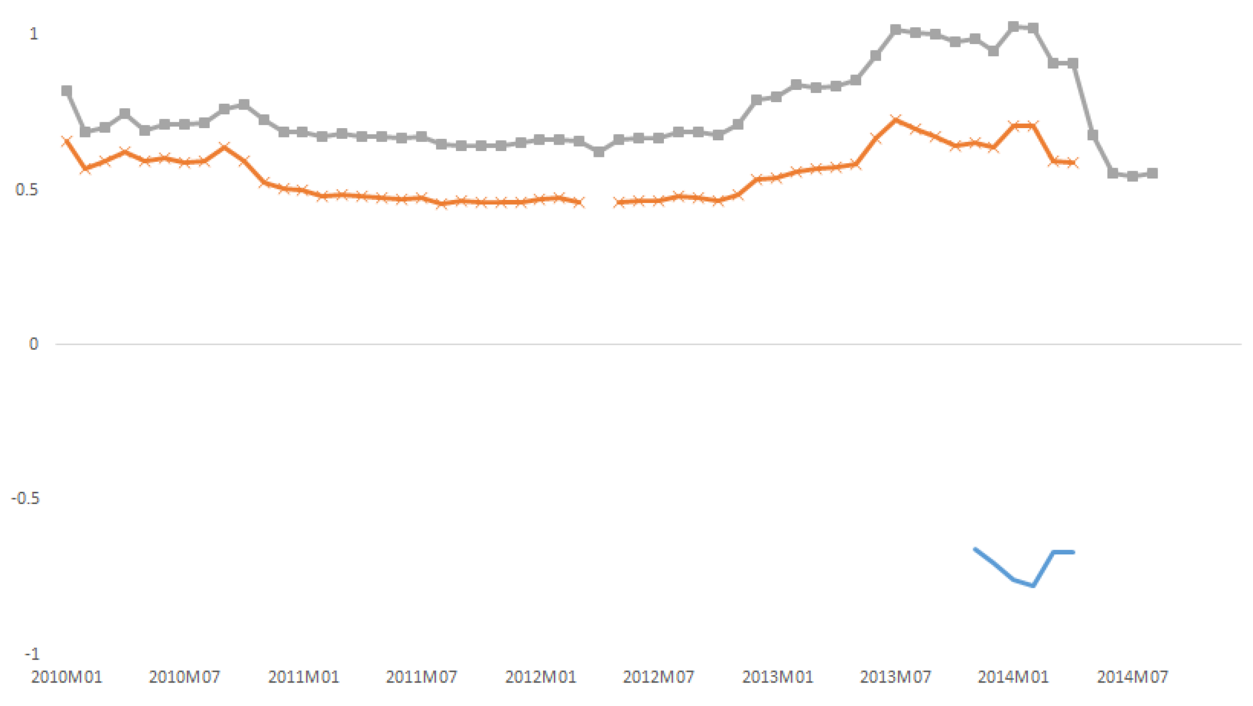
We now present some robustness checks of our lead-lag effect exercise. A rolling analysis was used to evaluate the stability of the parameters identifying the periods where the interaction between the two different segments of the market was more intense. Rolling analysis is also useful to study if and how the direction of the interaction changes over time. Finally, with the rolling analysis, we could examine the evolution of the autoregressive coefficients through time. The VAR model was estimated using a 60 month window (close to the 2000 day estimation window of DeMiguel et al. (2014)) testing along side the significance of the coefficients. In Figure 1, we present the time path of the estimated autoregressive coefficients and interaction terms. The gaps indicate the periods where they were not statistically significant. The large cap autoregressive coefficient ${\varphi }_{11}$ was statistically significant for almost the entire sample period until August 2014. The estimates of ${\varphi }_{11}$ were quite variable, indicating that the market trend in the large cap index was not constant over time. The joint conditions ${\varphi }_{11}$, ${\varphi }_{22}>0$ were needed to test for momentum, which in our case were eliminated to test that ${\varphi }_{11}>0$, since ${\varphi }_{22}$ was not significant in our benchmark model. It was apparent that the coefficient ${\varphi }_{11}$ was statistically positive for the entire sample period, highlighting the existence of momentum in the large cap segment of the market. The small cap interaction term ${\varphi }_{12}$ was statistically significant for the sample periods ending in November 2013 to April 2014, implying that the large cap index returns were affected by the lagged small cap index returns for a very short period. On the other hand, the interaction term of the lagged large cap return index on the small cap index return was statistically significant for almost the entire period ending in January 2010 to April 2014, with the exception of the period March 2012–May 2012.

4. Systemic Risk and Network Measures

The number of systemic risk definitions is vast, and the underlying idea is either based on the market’s efficiency, and therefore the information dispersion, or on the information coming from market data (e.g., accounting data). One prominent example of the market data based measure is the marginal expected shortfall (MES) of Acharya et al. (2017). In our analysis, we used MES and some variations of it.

4.1. Marginal Expected Shortfall

Consider the bivariate vector $r_t={(r_{i,t},r_{m,t})}^{\prime }$ of the i^th financial institution returns and of its reference market, m, at time t. Based on the expected shortfall, which is, in other words, the tail conditional expectation of Artzner et al. (1999), Acharya et al. (2017) introduced the marginal expected shortfall (MES) to capture the marginal contribution of the $i^{\mathrm{th}}$ institution to the risk of the financial system, defined as:

$$ME{S}_{i,t}(C)=\frac{\partial E{S}_{m,t-1}(C)}{\partial y_i}=-E\left[r_i\right|r_{m,t}\le C]$$

(4)

where $y_i$ is the weight of the $i^{\mathrm{th}}$ financial institution in the total portfolio $r_{m,t}={\sum }_i{y}_{i,t}{r}_{i,t}$ and C is a threshold that defines the distress event examined. Institutions with higher MES are the ones contributing the most to the market decline; hence, they are more likely to be systemically risky. Given our global dataset, we would be able to identify global systemically important financial institutions by estimating an institution’s capital shortfall in the case of a worldwide shock. In the aspect of the “cause and effect”, MES is on the “cause” side, in the sense that it is calculated assuming that the market index is already at the tail; therefore, MES captures the “effect” the later has, on the systemic risk of the stock. The aggregate MES is interpreted as the marginal expected shortfall of the returns of a portfolio consisting of individual banks’ equities when the market returns fall below a certain threshold level. In our implementation of MES, we used the dynamic conditional correlation to take into account the increase in volatility during crisis times. To this aim, we followed Brownlees and Engle (2012) and Engle (2012), who employed a bivariate GARCH model for the demeaned returns process, based on a capital asset pricing model (CAPM).

Let H be the variance-covariance matrix of $r_t={(r_{i,t},r_{m,t})}^{\prime }$, Brownlees and Engle (2012). Engle (2012) proposed that:

$$r_t=H_t^{1{/}_2}{ϵ}_t,$$

(5)

where ${ϵ}_t=({ϵ}_{m,t},{\eta }_{i,t})$ represents a vector of zero mean innovations, and:

$$H_t=\left(\begin{array}{cc}{\sigma }_{m,t}^2& {\sigma }_{m,t}{\sigma }_{i,t}{\rho }_{i,t}\\ {\sigma }_{m,t}{\sigma }_{i,t}{\rho }_{i,t}& {\sigma }_{i,t}^2\end{array}\right)$$

(6)

where ${\sigma }_{m,t}$ is the standard deviation of the reference market returns, ${\sigma }_{i,t}$ is the standard deviation of the financial institution’s returns, and ${\rho }_{i,t}$ is its correlation with the reference market returns. To estimate $H_t$, we used the dynamic conditional correlation model of Engle (2002) and Engle and Sheppard (2001). Under the model structure described by (5) and (6)6 and the definition of MES, it is shown that:7

$$\begin{array}{c}\hfill ME{S}_{i,t}(C)=E_{t-1}(r_{i,t}|r_{m,t}<C)=E_{t-1}({\sigma }_{i,t}{\rho }_{i,t}{\epsilon }_{m,t}+{\sigma }_{i,t}\sqrt{1-{\rho }_{i,t}^2}{\eta }_{i,t}|{\epsilon }_{m,t}<\frac{C}{{\sigma }_{m,t}})\\ \hfill ME{S}_{i,t}(C)={\sigma }_{m,t}{\rho }_{i,t}{E}_{t-1}({\epsilon }_{m,t}|{\epsilon }_{m,t}<\frac{C}{{\sigma }_{m,t}})+{\sigma }_{i,t}\sqrt{1-{\rho }_{i,t}^2}{E}_{t-1}({\eta }_{i,t}|{\epsilon }_{m,t}<\frac{C}{{\sigma }_{m,t}}).\end{array}$$

(7)

The last relationship states that MES is a weighted function of the tail expectation of the standardized market residual and the tail expectation of the standardized idiosyncratic financial institution’s residual, measuring the vulnerability of the financial institution i to the systemic risk originated from the financial market $m,$ given that the market returns are less than an assumed threshold C. The intuition behind higher values of MES is that the more vulnerable the institution is to systemic risk, the higher is its contribution to the risk of the financial system. Benoit et al. (2017) showed that MES and the systematic risk of the financial institution are proportional, that is:

$$\begin{array}{c}\hfill ME{S}_{i,t}(C)={\beta }_{i,t}{E}_{t-1}(r_{m,t}|r_{m,t}<Va{R}_{m,t}(C))={\beta }_{i,t}E{S}_{m,t}(C),\end{array}$$

(8)

where ${\beta }_{i,t}={\rho }_{i,t}\frac{{\sigma }_{i,t}}{{\sigma }_{m,t}}$ is the time-varying beta and $E{S}_{m,t}(C)$ is the expected shortfall of the market.

The functional form of MES implies that it can be aggregated, resulting in an aggregate measure, which is interpretable as the marginal expected shortfall of the return of the portfolio of stocks conditional on the market returns being below a certain threshold level.

4.2. Network Marginal Expected Shortfall

In highly correlated markets, such as financial systems, it could be very well the case that the correlation between the market and the institution returns contains other effects, for example, the correlation of the institution with other institutions or the correlation of the market with other institution returns. To remove “spurious” effects, which may bias the relationship between the institution and the market returns, we replaced marginal correlations with partial correlations: the correlations between the residuals from the regression of the institution returns on all other institution returns and the residuals from the regression of the market returns on all other institutions. In this way, we obtained a “netted” estimate of H, not biased by spurious effects, and consequently, a “netted” estimate of MES. We followed the definition of NetMES as introduced by Hashem and Giudici (2016) to take interconnectedness into account in the estimation of MES, and the partial correlations, ${\rho }_{ij.V}$, are calculated by:

$$\begin{array}{c}\hfill {\rho }_{ij.V}=corr({\epsilon }_{X_i|X_{V\backslash \left\{j\right\}}},{\epsilon }_{X_j|X_{V\backslash \left\{i\right\}}}).\end{array}$$

where ${\epsilon }_{X_i|X_{V\backslash \left\{j\right\}}}$ are residuals of the regression of $X_i$ on all other variables excluding $X_j$ and ${\epsilon }_{X_j|X_{V\backslash \left\{i\right\}}}$ are the residuals of the regression of $X_j$ on all other variables excluding $X_i$. The partial correlation coefficient allows measuring the additional contribution of variable $X_j$ to the variability of $X_i$ that is not already explained by the other variables, and vice versa. In our setting, we regressed the market index and institution $i_1$ to the rest of institutions returns to extract the residuals ${ϵ}_{i_{1}t}$ and ${ϵ}_{mt}$, that is:

$$\left\{\begin{array}{cc}\hfill r_{m,t}& =a_1+{\beta }_2{r}_{i_2,t}+\dots +{\beta }_n{r}_{i_n,t}+{\epsilon }_{i_1,t}\hfill \\ \hfill r_{i_1,t}& =a_1+{\beta }_2{r}_{i_2,t}+ldots+{\beta }_n{r}_{i_n,t}+{\epsilon }_{m,t}\hfill \end{array}\right.$$

(9)

and then, we obtained the partial correlation, that is ${\rho }_{m,i_1}=corr({\epsilon }_{m,t},{\epsilon }_{i_1,t})$. We repeated this extraction process for each pair of market and institution returns $(r_{mt},r_{it})$, which are inserted in (8), to obtain the variance-covariance matrix, H, and consequently the NetMES.

4.3. Bayesian Network Marginal Expected Shortfall

A network is comprised of a set of financial institutions, in which each institution represents a node. Assuming a multivariate Gaussian model for the time series observations of N financial agents, the linkages between the nodes can be described by an adjacency matrix A that has an $N\times N$ dimension with elements $a_{i,j}$, in which $a_{i,j}=1$ when two nodes are correlated and $a_{i,j}=0$ when they are not correlated. Partial correlations can be estimated assuming that the same observations follow a graphical Gaussian model, in which the variance-covariance matrix $\mathsf{\Sigma }$ is constrained by the conditional independence described by a graph (see e.g., Lauritzen (1996)).

More formally, let $x=\left(x_1,ldots,x_N\right)\in R^N$ be an N-dimensional random vector distributed according to a multivariate normal distribution ${\mathcal{N}}_N\left(\mu ,\mathsf{\Sigma }\right)$. We assume throughout that the covariance matrix $\mathsf{\Sigma }$ is not singular. For an undirected graph, let $G=(V,E)$, with vertex set $V=\left\{1,ldots,N\right\}$ and edge set $E=V\times V$, a binary matrix, with elements $e_{ij}$, which describe whether pairs of vertices are (symmetrically) linked between each other ($e_{ij}=1$) or not ($e_{ij}=0$). If the vertices V of a graph are put in correspondence with the random variables $X_1,ldots,X_N$, the edge set E induces conditional independence on X via the so-called Markov properties (see, e.g., Lauritzen (1996)). More precisely, the pairwise Markov property determined by G states that for all $1\le i<j\le N$:

$$e_{ij}=0⟺X_i\perp X_j|X_{V\backslash \{i,j\}};$$

The absence of an edge between vertices i and j is equivalent to independence between the random variables $X_i$ and $X_j$, conditionally on all other variables $x_{V\backslash \{i,j\}}$.

In our context, all random variables are continuous, and it is assumed that $X\sim {\mathcal{N}}_N\left(0,\mathsf{\Sigma }\right)$. Let the elements of ${\mathsf{\Sigma }}^{-1}$, the inverse of the variance-covariance matrix, whose elements are indicated by $\left\{{\sigma }^{ij}\right\}.$ Whittaker (2009) proved that the following equivalence also holds:

$$X_i\perp X_j|X_{V\backslash \{i,j\}}⟺{\rho }_{ij.V}=0$$

where:

$${\rho }_{ij.V}=\frac{-{\sigma }^{ij}}{\sqrt{{\sigma }^{ii}{\sigma }^{jj}}}$$

denotes the $i{j}^{\mathrm{th}}$ partial correlation. It can also be shown that the partial correlation coefficient ${\rho }_{ij.V}$ is equal to the correlation of the residuals from the regression of $X_i$ on all other variables (excluding $X_j$) with the residuals from the regression of $X_j$ on all other variables (excluding $X_i$), as in the following:

$${\rho }_{ij.V}=({\epsilon }_{X_i|X_{V\backslash \left\{j\right\}}},{\epsilon }_{X_j|X_{V\backslash \left\{i\right\}}}).$$

In other words, the partial correlation coefficient measures the additional contribution of variable $X_j$ to the variability of $X_i$ not already explained by the others, and vice versa.

A graphical Gaussian model is a Gaussian distribution constrained by a set of partial correlations equal to zero, which corresponds to variables whose additional contribution is not statistically significant. Mathematically, by means of the pairwise Markov property, given an undirected graph $G=(V,E)$, a graphical Gaussian model can be defined as the family of all N-variate normal distributions ${\mathcal{N}}_N\left(0,\mathsf{\Sigma }\right)$ that satisfy the constraints induced by the graph on the partial correlations for all $1\le i<j\le N$, as follows:

$$e_{ij}=0⟺{\rho }_{ij.V}=0.$$

In practice, the available data are used to test which partial correlations are different from zero at the chosen significance level threshold $\alpha$. A drawback of this approach is that results are conditional on a fixed graphical structure. To overcome this problem, we employed a Bayesian model averaging approach, where the estimates were the averages of those coming from the different graphical structure, each with a weight that corresponded to the Bayesian posterior probability of the corresponding graph.

For the purpose of a Bayesian application, the first task was to derive the likelihood of a graphical network and specify an appropriate probability distribution over all graphical networks. For a given a graph G, we considered a sample X of size n from a Gaussian probability distribution $P={\mathcal{N}}_N(0,\mathsf{\Sigma })$, and let S be the observed variance-covariance matrix that estimates $\mathsf{\Sigma }$. The graph G has a defined subset of vertices $A\subset N$, in which ${\mathsf{\Sigma }}_A$ denotes the variance-covariance matrix of the variables in $X_A$ and has $S_A$ as the corresponding observed variance-covariance submatrix. When the graph G is decomposable, the likelihood of the data, under the graphical Gaussian model specified by P, nicely decomposes as follows (see, e.g., Giudici and Spelta (2016)):

$$p(x|\mathsf{\Sigma },G)=\frac{{\prod }_{c\in \mathcal{C}}p(x_C|{\mathsf{\Sigma }}_C)}{{\prod }_{s\in \mathcal{S}}p(x_S|{\mathsf{\Sigma }}_S)}$$

where C and S respectively denote the set of cliques and separators of the graph G, and:

$$P(x_C|{\mathsf{\Sigma }}_C)={(2\pi )}^{-\frac{n*\left|C\right|}{2}}|{\mathsf{\Sigma }}_C{|}^{-n/2}exp[-1/2tr\left(S_C\left({\mathsf{\Sigma }}_C\right){}^{-1}\right)]$$

and similarly for $P(x_S|{\mathsf{\Sigma }}_S)$. A convenient prior for the parameters of the above likelihood is the hyper inverse Wishart distribution. It can be obtained from a collection of clique specific marginal inverse Wishart distributions as follows:

$$l(\mathsf{\Sigma })=\frac{{\prod }_{c\in \mathcal{C}}l({\mathsf{\Sigma }}_C)}{{\prod }_{s\in \mathcal{S}}l({\mathsf{\Sigma }}_S)}$$

where $l({\mathsf{\Sigma }}_C)$ is the density of an inverse Wishart distribution, with hyper-parameters $T_C$ and $\alpha$, and similarly for $l({\mathsf{\Sigma }}_S)$. For the definition of the hyper-parameters, here we follow Giudici and Spelta (2016), and let $T_C$ and $T_S$ be the sub-matrices of a larger matrix $T_0$ of dimension $N\times N$, obtained in correspondence with the two complete sets of vertices C and S, assuming that $\alpha >N$. To complete the prior specification, for $P(G)$, we consider a uniform prior over all possible graphical structures. Dawid and Lauritzen (1993) showed that, under the previous assumptions, the posterior distribution of the variance-covariance matrix $\mathsf{\Sigma }$ is a hyper Wishart distribution with $\alpha +N$ degrees of freedom and a scale matrix given by:

$$T_n=T_0+S_n$$

where $S_n$ is the sample variance-covariance matrix. This result can be used for quantitative learning on the unknown parameters, for a given graphical structure. In addition, Dawid and Lauritzen (1993) showed that the proposed prior distribution can be used to integrate the likelihood with respect to the unknown random parameters, obtaining the so-called marginal likelihood of a graph, which is the main metric for structural learning. Such a marginal likelihood is equal to:

$$P\left(x|G\right)=\frac{{\prod }_{c\in \mathcal{C}}p(x_C)}{{\prod }_{s\in \mathcal{S}}p(x_S)}$$

in which:

$$p\left(x_C\right)={(2\pi )}^{-\frac{n*\left|C\right|}{2}}\frac{k\left(\left|C\right|,\alpha +n\right)}{k\left(\left|C\right|,\alpha \right)}\frac{det{\left(T_0\right)}^{\alpha /2}}{det{\left(T_n\right)}^{(\alpha +n)/2}}$$

where $k(·)$ is the multivariate gamma function, given by:

$$k_p\left(a\right)={\pi }^{\frac{p\left(p-1\right)}{4}}{\prod }_{j=1}^p\mathsf{\Gamma }\left(a+\frac{1-j}{2}\right)$$

Assume that we have several possible graphs, say $n(G)$, and that they are equally likely a prior, so that the probability of $P(G)$ is:

$$P(G)=\frac{1}{\left|G\right|}$$

By Bayes rule, the posterior probability of a graph is given by:

$$P\left(G|x\right)\propto P\left(x|G\right)P\left(G\right)$$

and therefore, since we assume a uniform prior over the graph structures, maximizing the posterior probability is equivalent to maximizing the marginal likelihood. For graphical model selection purposes, we searched in the space of all possible graphs for the structure such that:

$$G^{*}=arg\underset{G}{max}P\left(G|x\right)\propto arg\underset{G}{max}P\left(x|G\right).$$

A Bayesian model averaging approach does not force conditioning inferences on the (best) model chosen. If we assume that the network structure G is random and we assign a prior distribution on it, we derive inference on unknown parameters as model averages to all possible graphical structures, with weights that correspond to the posterior probabilities of each network. This derives from the application of Bayes’ theorem, as follows:

$$P(\mathsf{\Sigma }|X)=P(\mathsf{\Sigma }|x,G)P(G|x).$$

Note that, in many real problems, the number of possible graphical structures could be very large, and we may need to restrict the number of models to be averaged. This can be done efficiently, for example, following a simulation based procedure for model search, such as Markov chain Monte Carlo (MCMC) sampling. In our context, given an initial graph, the algorithm samples a new graph using a proposal distribution. To guarantee irreducibility of the Markov chain, we followed Giudici and Spelta (2016) to test whether the proposed graph was decomposable. The newly sampled graph was then compared with the old graph, calculating the ratio between the two marginal likelihoods; if the ratio was greater than a predetermined threshold (acceptance probability), the proposal was accepted, otherwise, it was rejected. The algorithm continued until practical convergence was reached.

Following Hashem and Giudici (2016), we average NetMES as follows:

$$E(MES|x)=\sum _{g}E(MES|x,g)P(g|x),$$

(10)

where x represents the observed data evidence and g a specific network model. The estimated $E(MES|X)$ is referred to as a Bayesian Network based marginal expected shortfall measure (Bayesian NetMES).

4.4. Centrality Measures

Centrality measures address the question of who is the most important in the network. There are many answers to this question, depending on what we mean by importance. There are a vast number of different centrality measures. We used the most popular ones, like closeness, node degree, eigenvector, and betweenness. Closeness calculates the inverse of the fairness, or the inverse of the sum of shortest paths between a node and all other nodes, and thus, it allows detecting nodes that are best placed to influence the entire network quickly and that represent influence or information broadcasters. Node degree centrality assigns the node importance score based on the summation of the number of links a node has with others. Eigenvector centrality can identify nodes that possess influence over the whole network, not just those directly connected to it; in other words, eigenvector centrality is a measure of the overall influence extent of a specific node on others in a network, this measure assigns scores to nodes based on the concept that connections to high-score nodes contribute more to the score of the specified node than equal connections to low-score nodes. Betweenness centrality measures the number of times a node lies on the shortest path between other nodes, or the number of times a node acts as a bridge along the shortest path between others. It was introduced as a measure for quantifying the control of a human of the communication between other humans in a social network by Linton Freeman. Intuitively, betweenness measures a node’s influence on the information flow circulating through the social network, under the assumption that the flow follows shortest paths.

5. Findings and Discussion

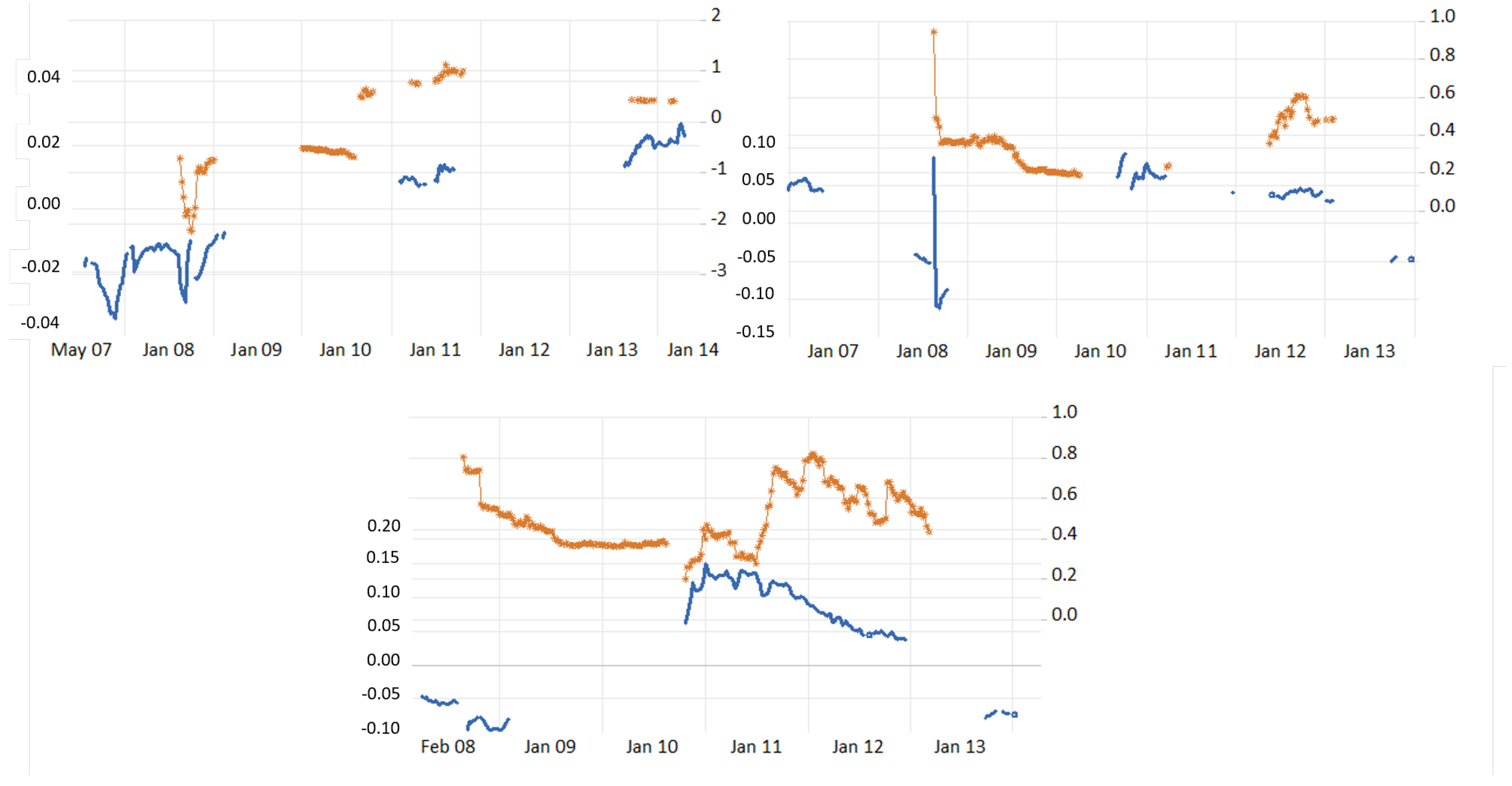
We examined the lead-lag relationship of the survived financial institutions systemic risk measures by estimating the regression (1) using a two year rolling window. Figure 2 shows the evolution of the interaction terms ${\varphi }_{12}$ and ${\varphi }_{21}$ identifying the periods where the large cap survived financial institutions led the small cap8 in terms of systemic risk, and vice versa. It is notable that the interaction terms did not show a pattern like that of the lead-lag behavior of the financial returns in Figure 1. The MES of the small cap led the MES of the large cap from 24 August 2007 until 12 September 2009. Moreover, the negative sign of the ${\varphi }_{21}$ implied a decrease of the MES of the large cap when an increase of the MES of small cap occurred. It is also worth noticing that the magnitude of ${\varphi }_{12}$ was 100 times larger than ${\varphi }_{21}$. The MES behavior was interpreted with the crisis effect on the stock market returns behavior. Sandoval and Franca (2012) showed that an increase in market volatility led to an increase in the correlation between market assets, indicating the increase in the level of uniform behavior of market participants during crisis times. This being said, and knowing that MES estimation was not size dependent, nevertheless, it captured the increase in the small cap volatility during crisis times, which may be interpreted in terms of both capitalization and liquidity availability. Terraza (2015) showed that the capital adequacy degree declined during 2008, but there was an increase in capitalization and liquidity after that except for small banks in 2011 and 2012. In addition, Ding and Sickles (2018) pointed out a positive relation between capital and risk adjustments of large banks that held low capital buffers; however, they pointed out a negative relation between capital and risk adjustments for small banks with low capital buffers. The decrease of the large cap MES upon the increase in MES of the small cap along with the larger magnitude of the small cap MES could be foreseen as a positive improvement in large cap returns compared to small ones, which may be viewed as a change in the market expectations for large cap risks in relation to governmental bailout plans. Brewer and Klingenhagen (2010) showed that large banks’ stock prices that were classified as too big to fail (TBTF) performed better in the short run than smaller banks in the USA as a reaction to the U.S. government bailout programs.

The evolution of NetMES showed that the small-large lead-lag relationship was present from 19 September 2008, until 11 November 2008. The coefficient ${\varphi }_{21}$ was mostly negative as in the case of MES. Again, the magnitude of the interaction term ${\varphi }_{12}$ was quite larger than the ${\varphi }_{21}.$ The results of NetMES were inline with MES, but were limited to a shorter time span that was located within the heart of the global financial crisis of 2008. Originally, MES was estimated using correlations that captured both direct and indirect relationships; mainly as it provided the degree of association between the financial institution and the specified index without controlling for the effects from other financial institutions, while NetMES was estimated using partial correlations that considered only the direct relationships; as the effect of the set of other financial institutions was removed. Therefore, NetMES excluded the impact from other institutions upon the computation of the co-movements between the selected institution and the market index. This estimation method of NetMES imposed sparsity on the financial network structure whenever the partial correlation coefficient was insignificant, indicating that the corresponding financial institution did not directly contaminate others. The lead-lag relationship was also confirmed by the Bayesian NetMES between the large and the small cap financial institutions from 10 October 2008, until 6 March 2009. From 3 December 2010–25 January 2013, the lead-lag relationship was supported again. The difference in Bayesian NetMES in terms of the longer periods of the lead-lag results referred to the model specification, which represented an averaging mechanism over the systemic risk measure. The Bayesian model allowed us to examine the network structure while tacking into account the model uncertainty.

To reveal additional features of the evolution of the systemic risk level of financial institutions, we continued by examining the sub-industries. A careful examination of Figure 3 reveals that all the systemic risk indicators sharply increased their magnitude in 2009. In particular, for the large cap survived financial institutions, the MES showed that DB and TMF experienced the highest increase. The NetMES and Bayesian NetMES showed that except the aforementioned sub-industries, also DCM and IBB increased sharply. Furthermore, a notable feature was the negative signs of MES in the case of the AMC, DB, RB, and TMF. This suggested that the financial sub-industries responded negatively to the downfall of the market. Laopodis (2016) pointed out the presence of a significant explanatory power from industry to stock market returns, indicating the consistent informational leadership from the financial industry to other industries. When NetMES and the Bayesian NetMES were considered, the negative values were present mainly for AMC and TMF. Additionally, MES for DB and TMF started to increase again in 2012 (Greek default) and in 2013 reached another peak. In the case of NetMES and Bayesian NetMES, there was a peak of the systemic risk measures for the IBB sub-industry.

For the small cap, the systemic risk measures reached their highs in late 2008–early 2009. The sub-industries systemic risk change in magnitude could be interpreted in relation to the level of the financial leverage ratio9. It was shown that TMF was the one that had the highest leverage increase during the crisis period, followed by DB. It is noticeable that the magnitude change of NetMES and Bayesian NetMES was affected by the magnitude change of leverage. This indicated that the change magnitude within the netted financial risk network was leverage driven, which captured the specificity of the subprime mortgage crisis. This feature infused the debate on the MES rational concept, in which the MES was argued to be close to the too interconnected to fail (TITF) logic rather than the too big to fail (TBTF) one. This logical relation could also be noticed from the sub-industries market capitalization (see

Table A3. Financial leverage and market capitalization of survived financial institutions per sub-industry (GICS). Panels A and C provide leverage of the large and small cap survived financial institutions per sub-industry calculated over two year sub periods from 2005–2014. Panels B and D provide the market capitalization of the large and small cap survived financial institutions calculated like the financial leverage.

Panel A: Financial Leverage of Large-Cap Survived Financial Institutions (Average Per Period)
Sub-industry	1/1/2005–12/31/2006	1/1/2007–12/31/2008	1/1/2009–12/31/2010	1/1/2011–12/31/2012	1/1/2013–12/31/2014
Asset Management & Custody Banks (AMC)	1.44	1.82	1.77	1.49	1.41
Diversified Banks (DB)	2.80	3.75	5.67	6.23	4.68
Diversified Capital Markets (DCM)	2.65	3.77	3.76	4.04	4.24
Investment Banking & Brokerage (IBB)	3.34	4.13	4.97	7.13	5.51
Regional Banks (RB)	1.81	2.28	2.92	2.58	2.36
Thrifts & Mortgage Finance (TMF)	5.75	20.64	144.54	382.19	82.07
Panel B: Market Capitalization of Large-Cap Survived Financial Institutions (Total Per Period. Numbers in Billion U.S. Dollars)
Sub-industry	1/1/2005–12/31/2006	1/1/2007–12/31/2008	1/1/2009–12/31/2010	1/1/2011–12/31/2012	1/1/2013–12/31/2014
Asset Management & Custody Banks (AMC)	212,536	271,262	197,192	219,003	289,875
Diversified Banks (DB)	2,092,360	2,278,660	1,944,820	2,231,659	2,941,330
Diversified Capital Markets (DCM)	88,566	109,625	77,923	77,553	95,089
Investment Banking & Brokerage (IBB)	210,996	216,106	174,965	151,316	219,165
Regional Banks (RB)	342,808	300,445	228,424	257,018	322,905
Thrifts & Mortgage Finance (TMF)	125,271	90,002	36,084	37,321	67,174
Panel C: Financial Leverage of Small-Cap Survived Financial Institutions Per Sub-Industry(Average Per Period)
Sub-industry	1/1/2005–12/31/2006	1/1/2007–12/31/2008	1/1/2009–12/31/2010	1/1/2011–12/31/2012	1/1/2013–12/31/2014
Asset Management & Custody Banks (AMC)	2.16	2.43	2.61	1.78	1.60
Diversified Banks (DB)	5.09	8.14	11.71	7.82	6.89
Investment Banking & Brokerage (IBB)	1.48	1.78	1.78	3.13	4.02
Regional Banks (RB)	1.78	2.31	3.54	2.99	2.23
Thrifts & Mortgage Finance (TMF)	5.36	27.92	56.08	23.04	10.45
Panel D: Market Capitalization of Small-Cap Survived Financial Institutions(Total Per Period. Numbers in Billion U.S. Dollars)
Sub-industry	1/1/2005–12/31/2006	1/1/2007–12/31/2008	1/1/2009–12/31/2010	1/1/2011–12/31/2012	1/1/2013–12/31/2014
Asset Management & Custody Banks (AMC)	4634	5834	3727	3794	4039
Diversified Banks (DB)	4034	6734	6180	5345	5331
Diversified Capital Markets (DCM)	2077	2440	857	680	600
Investment Banking & Brokerage (IBB)	5857	7802	6015	5250	5904
Regional Banks (RB)	19,721	17,564	11,918	13,117	16,876
Thrifts & Mortgage Finance (TMF)	3468	2506	1690	1988	2632

) showing that large DB had the highest total market capitalization for the overall and the crisis periods, and the highest change in magnitude during the crisis period, while the change was a decrease for TMF, consistent with its higher leverage increase relative to its smaller capitalization. Several theories support the view that large and complex banks contribute to systemic risk. In the TBTF hypothesis, the regulators were reluctant to close or unwind large and complex banks, resulting in moral hazard behavior. As a result, the leading banks took on excessive risks in the expectation of government bailouts (Farhi and Tirole 2012).

Subsequent to our initial approach, we will tackle the issue in terms of the individual institution’s system risk importance capturing their vulnerability to a market-wide systemic shock10. The rankings were based on the MES, the NetMES, and the Bayesian NetMES, respectively. We compared the three rankings by implementing a Kolmogorov–Smirnov test that compared their corresponding cumulative distributions. For the large cap, we rejected at 5% the null hypotheses in favor of the alternative that the MES of the large cap institutions was larger than the NetMES. The null hypothesis was not rejected when we compared the distributions of NetMES and the Bayesian NetMES. For the small cap, the MES and NetMES were found again significantly different. The null hypothesis was not rejected for NetMES and Bayesian NetMES, and MES and Bayesian NetMES. Additionally, we examined the autocorrelation structure of the series. Kendall’s $\tau$ between the spot and the lagged value of the systemic risk measures equaled 0.7488 (MES), 0.6005 (NetMES), and 0.5631 (Bayesian NetMES) for the large cap survived financial institutions and 0.8856 (MES), 0.6566 (NetMES), and 0.6611 (Bayesian NetMES), indicating strong autocorrelation of the MES values, and consequently, the more reluctant to changes rankings compared to NetMES and Bayesian NetMES values.

Next, we followed Benoit et al. (2013), who used the top ten financial institutions by systemic risk importance, which accounted for 10% of their sample, and we proceeded with our analysis using the top six the financial institutions, which accounted for 12.84% of the total number of the survived financial institutions11. For each sub-period, the institutions and the countries are provided in a dot joint ticker country column (Ticker.Country).

Table 1. Top six systemically important large cap survived financial institutions. In the fourth column, “3”: systemically important by all three systemic risk measures (MES, NetMES, Bayesian NetMES); “2” systemically important by two of the three systemic risk measures; “1”: systemically important by one of the three systemic risk measures.

Financial Institution	Sub-Industry	Country
Legg Mason Inc.	AMC	UNITED STATES	3
Jafco Co Ltd.	AMC	JAPAN	3
Santander Chile Holding SA	AMC	CHILE	3
VP Bank AG	AMC	LIECHTENSTEIN	3
Vontobel Holding AG	AMC	SWITZERLAND	3
Alpha Bank AE	DB	GREECE	3
Hellenic Bank PCL	DB	CYPRUS	3
Credicorp Ltd.	DB	PERU	3
Natixis SA	DCM	FRANCE	3
China Everbright Ltd.	DCM	HONG KONG	3
Investec Ltd.	DCM	SOUTH AFRICA	3
Macquarie Group Ltd.	DCM	AUSTRALIA	3
Mirae Asset Daewoo Co Ltd.	DCM	SOUTH KOREA	3
Deutsche Bank AG	DCM	GERMANY	3
Tokai Tokyo Financial Holdings Inc.	IBB	JAPAN	3
Goldman Sachs Group Inc/The, TD Ameritrade Holding Corp	IBB	UNITED STATES	3
Daiwa Securities Group Inc.	IBB	JAPAN	3
Caisse Regionale de Credit Agricole Mutuel de Paris et d’Ile-de-France	RB	FRANCE	3
Paragon Banking Group PLC	TMF	GREAT BRITAIN	3
MGIC Investment Corp, TrustCo Bank Corp NY, New York Community Bancorp Inc, Capitol Federal Financial Inc.	TMF	UNITED STATES	3
MLP SE	AMC	GERMANY	2
Allied Irish Banks PLC	DB	IRELAND	2
China Banking Corp	DB	PHILIPPINES	2
Swedbank AB	DB	SWEDEN	2
Investment Technology Group Inc.	IBB	UNITED STATES	2
Capital Securities Corp	IBB	TAIWAN	2
Caisse Regionale de Credit Agricole Mutuel Alpes Provence	RB	FRANCE	2
Oldenburgische Landesbank AG	RB	GERMANY	2
Public Financial Holdings Ltd.	RB	HONG KONG	2
Daishi Bank Ltd/The, Nishi-Nippon City Bank Ltd/The	RB	JAPAN	2
Federal Home Loan Mortgage Corp	TMF	UNITED STATES	2
Federated Investors Inc.	AMC	UNITED STATES	2
Rathbone Brothers PLC	AMC	GREAT BRITAIN	2
RHB Capital Bhd	DB	MALAYSIA	2
Bank Maybank Indonesia Tbk PT	DB	INDONESIA	2
CIMB Group Holdings Bhd	DB	MALAYSIA	2
Bank Cler AG	DB	SWITZERLAND	2
KB Securities Co Ltd.	IBB	SOUTH KOREA	2
Minato Bank Ltd/The	RB	JAPAN	2
Popular Inc.	RB	PUERTO RICO	2
First Midwest Bancorp Inc/IL, Synovus Financial Corp, UMB Financial Corp, 1st Source Corp	RB	UNITED STATES	2
Bank of America Corp	DB	UNITED STATES	1
Scotiabank Peru SAA	DB	PERU	1
TMB Bank PCL	DB	THAILAND	1
Mediobanca Banca di Credito Finanziario SpA	DB	ITALY	1
AFFIN Holdings Bhd	DB	MALAYSIA	1
BMCE Bank	DB	MOROCCO	1
Astoria Financial Corp	TMF	UNITED STATES	1
Aberdeen Asset Management PLC	AMC	GREAT BRITAIN	1
KBC Group NV	DB	BELGIUM	1
State Bank of India	DB	INDIA	1
BGC Partners Inc.	IBB	UNITED STATES	1
Marusan Securities Co Ltd.	IBB	JAPAN	1
BB&T Corp	RB	UNITED STATES	1
Piraeus Bank SA	DB	GREECE	1

and

Table 2. Top six systemically important small cap survived financial institutions. In the fourth column, “3”: systemically important by all the three systemic risk measures (MES, NetMES, Bayesian NetMES); “2”: systemically important by two of the three systemic risk measures; “1”: systemically important by one of the three systemic risk measures.

Financial Institution	Sub-Industry	Country
180 Degree Capital Corp	AMC	UNITED STATES	3
Effecten-Spiegel AG, Deutsche Beteiligungs AG	AMC	GERMANY	3
FDG Kinetic Ltd.	AMC	HONG KONG	3
GSD Holding AS	DB	TURKEY	3
Bank Ochrony Srodowiska SA	DB	POLAND	3
Alandsbanken Abp	DB	FINLAND	3
Barclays Bank of Botswana Ltd.	DB	BOTSWANA	3
Oppenheimer Holdings Inc.	IBB	UNITED STATES	3
Banca Profilo SpA	IBB	ITALY	3
Charles Stanley Group PLC	IBB	GREAT BRITAIN	3
Toyo Securities Co Ltd.	IBB	JAPAN	3
Banestes SA Banco do Estado do Espirito Santo	RB	BRAZIL	3
Seacoast Banking Corp of Florida, FNCB Bancorp Inc.	RB	UNITED STATES	3
Locindus SA	TMF	FRANCE	3
Federal Agricultural Mortgage Corp, NASB Financial Inc, OceanFirst Financial Corp, Provident Financial Holdings Inc.	TMF	UNITED STATES	3
Street Capital Group Inc.	TMF	CANADA	3
Bear State Financial Inc.	TMF	UNITED STATES	3
Peregrine Holdings Ltd.	AMC	SOUTH AFRICA	2
Sparebanken Vest	DB	NORWAY	2
Asia Plus Group Holdings PCL	IBB	THAILAND	2
First United Corp, CommunityOne Bancorp	RB	UNITED STATES	2
Atinum Investment Co Ltd.	AMC	SOUTH KOREA	2
National Bank of Kuwait-Egypt SAE	DB	EGYPT	2
Lan & Spar Bank	DB	DENMARK	2
Berliner Effektengesellschaft AG	IBB	GERMANY	2
GronlandsBANKEN A/S	RB	GREENLAND	2
Capital City Bank Group Inc, Baylake Corp	RB	UNITED STATES	2
SHK Hong Kong Industries Ltd.	AMC	HONG KONG	1
KAS Bank NV	AMC	NETHERLANDS	1
Airesis SA	AMC	SWITZERLAND	1
Norvestia Oyj	AMC	FINLAND	1
Sparebanken Ost	DB	NORWAY	1
Takagi Securities Co Ltd.	IBB	JAPAN	1
Cie Financiere Tradition SA	IBB	SWITZERLAND	1
South China Financial Holdings Ltd.	IBB	HONG KONG	1
Bryn Mawr Bank Corp, Cascade Bancorp, Commercial National Financial Corp/PA, Peoples Financial Corp/MS, C&F Financial Corp, Independent Bank Corp/MI, First Community Bancshares Inc/VA, First South Bancorp Inc/NC, Financial Institutions Inc, Heritage Commerce Corp, HopFed Bancorp Inc, MainSource Financial Group Inc, Pacific Continental Corp, Sun Bancorp Inc/NJ	RB	UNITED STATES	1
Tsukuba Bank Ltd.	RB	JAPAN	1
Sachsenmilch AG	AMC	GERMANY	1
Peapack Gladstone Financial Corp	RB	UNITED STATES	1
First US Bancshares Inc.		UNITED STATES	1
KAF-Seagroatt & Campbell Bhd	IBB	MALAYSIA	1

summarize the financial institutions’ systemic importance assumed by at least one of the systemic risk measures examined (Analytically, the top six ranked institutions per sub-industry are provided in the Tables A.2–A.7 of (Arakelian et al. 2019)). From the tables above, if we focus on the financial institutions retained systemically important by all the measures, we obtained a list of companies that was consistent with what happened to them:

• In the United States, Legg Mason Inc. (LM.US) was one of the institutional investors that bore a huge loss when Bear Stearns collapsed, as the group held 11% of Bear Stearns, making the group the bank’s biggest shareholder. Legg Mason was also ranked among the most important institutions by Acharya et al. (2017), as well as Goldman Sachs, TD Ameritrade, and New York Community Bancorp for the period June 2006–June 2007 that the authors examined.
• In France, two prominent French financial institutions were among the most massively hit by the fear of contingent liabilities: Natixis, France’s fourth largest bank, also assumed systemically important, had announced a €1.2 billion write-down of exposure to bad U.S. mortgage debt. Natixis, a publicly-listed corporate and investment banking firm jointly controlled by Caisses d’ Epargne (the French Savings Banks group) and Banques Populaires, and Dexia, a French-Belgian bank specializing in the financing of municipalities. In both cases, the problems were related to their investments in bond insurers in the United States: CDC IXIS Financial Guaranty (CIFG) in the case of Natixis and Financial Security Assurance (FSA) in the case of Dexia12.
• In Germany, an investment-banking arm of Deutsche Bank deeply involved in toxic securities was found systemic by all measures. By some estimates, German banks at the outset of the crisis had an average ratio of debt to net worth of 52 to one compared with 12 to one in the U.S. Indeed, the U.S. Federal Reserve helped Deutsche Bank with $290 billion in mortgage securities.
• In South Africa, Investec Bank was systemically important by all the measures. Indeed, the British government was forced to act by injecting liquidity into financial markets through various schemes including a 50 billion Credit Guarantee Scheme in October 2008, in which Investec Bank was eligible to participate.

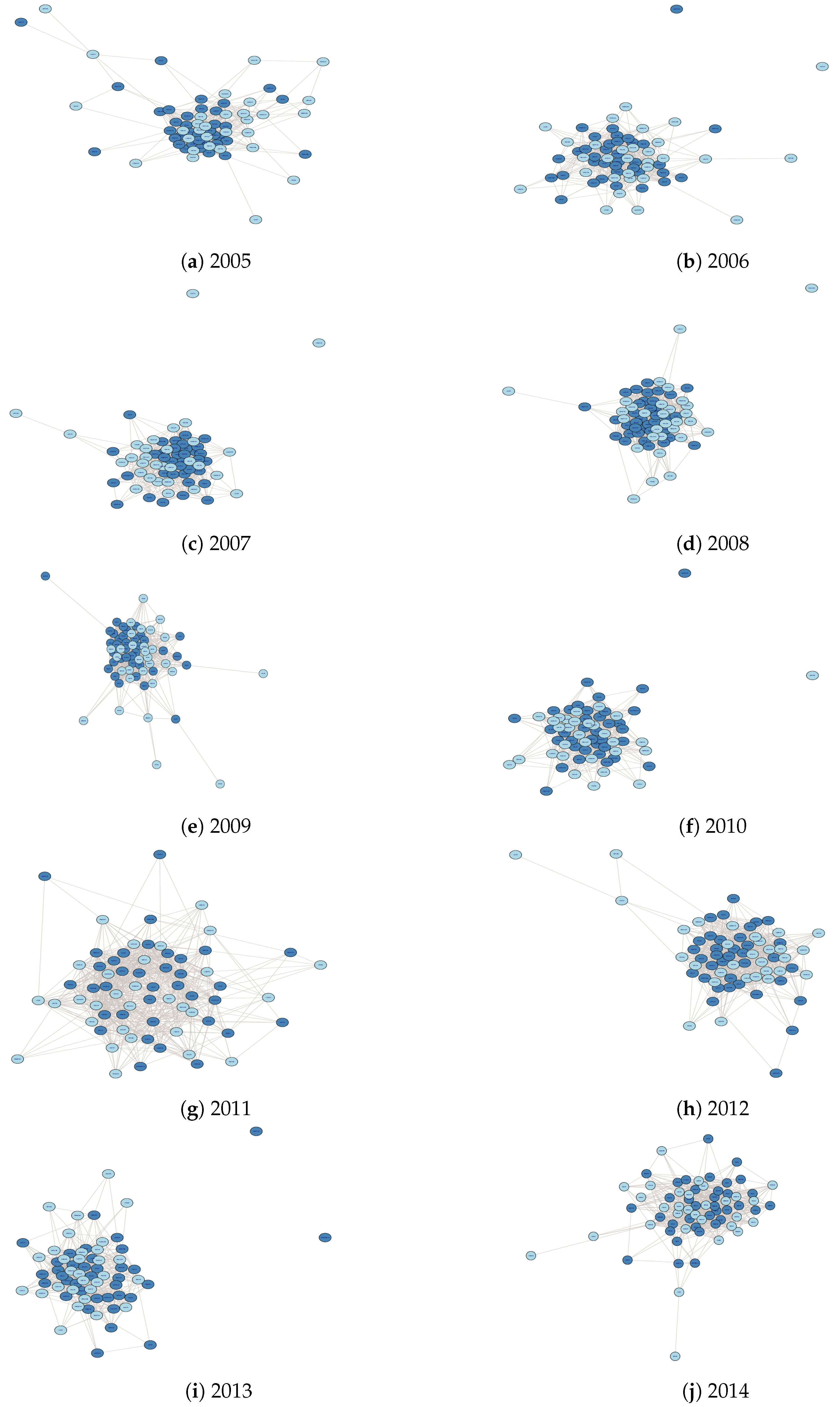
Subsequent to our initial objective was to investigate the network structure among the top six systemically important institutions per sub-industry. The network investigation aimed at modeling the interlinkages between the large and the small cap, revealing the channels through which shocks could propagate more widely in the financial system. Figure 4, Figure 5 and Figure 6 represent the yearly correlation networks for MES, NetMES, and Bayesian NetMES vectors of the top six financial institutions per sub-industry based on eigenvector centrality, providing a ranking of the nodes from the most to the least systemically important (the details of the graphs, as well as, the ranking provided by using other centrality measures are given summarized into centrality measures in

Table A4. Yearly centrality measures for MES correlation network of top 6 survived financial institutions per sub-industry provided in Figure 4. The table lists the highest 6 ranking institutions based on their centrality measure.

		Industry	Closeness		Industry	Degree		Industry	Eigenvector Centrality		Industry	Betweenness %
2005	SANTGRU.CI	L.AM	0.005181	LM.US	L.AM	14	OCFC.US	S.TMF	0.178653	OCFC.US	S.TMF	0.048558
	LM.US	L.AM	0.004975	SANTGRU.CI	L.AM	12	PGR.SJ	S.AMC	0.177352	ALBAV.FH	S.DB	0.047278
	MLP.GR	L.AM	0.004608	MLP.GR	L.AM	6	SANTGRU.CI	L.AM	0.174771	IMH.US	S.TMF	0.037376
	VONN.SW	L.AM	0.003922	8616.JP	L.IBB	4	FSBK.US	S.RB	0.173471	8614.JP	S.IBB	0.035849
	CAF.FP	L.RB	0.003861	BPI.PM	L.DB	4	SCB.TB	L.DB	0.171668	8616.JP	L.IBB	0.034817
	CHFC.US	L.RB	0.003861	KN.FP	L.DCM	4	MQG.AU	L.DCM	0.170623	GKG.SP	S.RCS	0.032493
2006	8595.JP	L.AM	0.005102	LM.US	L.AM	13	TPEIR.GA	L.DB	0.181499	GKG.SP	S.RCS	0.052294
	LM.US	L.AM	0.005051	MLP.GR	L.AM	9	CRAP.FP	L.RB	0.180081	FSBK.US	S.RB	0.051185
	MLP.GR	L.AM	0.004762	VPBN.SW	L.AM	6	CAF.FP	L.RB	0.169709	KNK.MK	S.IBB	0.035955
	VONN.SW	L.AM	0.004065	8601.JP	L.IBB	6	PGR.SJ	S.AMC	0.168861	CAF.FP	L.RB	0.029135
	BAC.US	L.DB	0.003906	ITG.US	L.IBB	5	SECH.KK	S.DCM	0.167201	IMH.US	S.TMF	0.026233
	SANTGRU.CI	L.AM	0.003876	8595.JP	L.AM	4	8616.JP	L.IBB	0.164756	CHIB.PM	L.DB	0.025356
2007	MLP.GR	L.AM	0.005291	8595.JP	L.AM	14	MTG.US	L.TMF	0.172005	TMB.TB	L.DB	0.055944
	8595.JP	L.AM	0.005181	SANTGRU.CI	L.AM	9	FCBC.US	S.RB	0.171019	CNS.TB	S.IBB	0.042395
	SANTGRU.CI	L.AM	0.004831	VPBN.SW	L.AM	7	CFFN.US	L.TMF	0.165398	OPY.US	S.IBB	0.034206
	LM.US	L.AM	0.004082	MLP.GR	L.AM	6	CHIB.PM	L.DB	0.165047	DXIL.IT	S.DB	0.033959
	BPSO.IM	L.DB	0.004082	LM.US	L.AM	5	165.HK	L.DCM	0.164251	AMTD.US	L.IBB	0.030148
	VPBN.SW	L.AM	0.003984	TMB.TB	L.DB	5	SBCF.US	S.RB	0.162894	BPSO.IM	L.DB	0.027496
2008	SANTGRU.CI	L.AM	0.00578	SANTGRU.CI	L.AM	12	GSDHO.TI	S.DB	0.140767	626.HK	L.RB	0.078572
	MLP.GR	L.AM	0.004975	ALBK.ID	L.DB	10	GKG.SP	S.RCS	0.139739	MLP.GR	L.AM	0.043968
	ALBK.ID	L.DB	0.004739	VPBN.SW	L.AM	9	NYCB.US	L.TMF	0.138752	GKG.SP	S.RCS	0.043732
	HB.CY	L.DB	0.004484	ALPHA.GA	L.DB	6	MTG.US	L.TMF	0.138549	GSDHO.TI	S.DB	0.041172
	INL.SJ	L.DCM	0.004329	INL.SJ	L.DCM	5	PGR.SJ	S.AMC	0.138138	EFS.GR	S.AMC	0.036526
	8601.JP	L.IBB	0.004329	8601.JP	L.IBB	5	SANTGRU.CI	L.AM	0.138068	KN.FP	L.DCM	0.032975
2009	VPBN.SW	L.AM	0.005435	VPBN.SW	L.AM	16	626.HK	L.RB	0.142476	626.HK	L.RB	0.020224
	LM.US	L.AM	0.004505	8595.JP	L.AM	7	OPY.US	S.IBB	0.141236	OPY.US	S.IBB	0.017514
	BAC.US	L.DB	0.004464	SWEDA.SS	L.DB	7	TRST.US	L.TMF	0.141071	TRST.US	L.TMF	0.018687
	BAP.US	L.DB	0.004464	BAC.US	L.DB	5	NYCB.US	L.TMF	0.140346	NYCB.US	L.TMF	0.013479
	8595.JP	L.AM	0.004167	ITG.US	L.IBB	5	MQG.AU	L.DCM	0.140346	MQG.AU	L.DCM	0.013479
	INL.SJ	L.DCM	0.004032	AIRE.SW	S.AMC	5	KA.NA	S.AMC	0.14023	KA.NA	S.AMC	0.013905
2010	8595.JP	L.AM	0.005587	8595.JP	L.AM	10	AF.US	L.TMF	0.174098	AF.US	L.TMF	0.021152
	SANTGRU.CI	L.AM	0.005128	VPBN.SW	L.AM	8	FBAK.US	L.RB	0.170886	FBAK.US	L.RB	0.027655
	VPBN.SW	L.AM	0.004695	SANTGRU.CI	L.AM	7	INL.SJ	L.DCM	0.170254	INL.SJ	L.DCM	0.026623
	ALPHA.GA	L.DB	0.004255	ALPHA.GA	L.DB	6	NYCB.US	L.TMF	0.169919	NYCB.US	L.TMF	0.016441
	DBK.GR	L.DCM	0.004219	8616.JP	L.IBB	6	165.HK	L.DCM	0.158964	165.HK	L.DCM	0.025424
	LM.US	L.AM	0.004219	LM.US	L.AM	5	KN.FP	L.DCM	0.158697	KN.FP	L.DCM	0.010844
2011	LM.US	L.AM	0.005525	LM.US	L.AM	10	6800.KS	L.DCM	0.152724	CAF.FP	L.RB	0.094042
	SANTGRU.CI	L.AM	0.004651	MLP.GR	L.AM	8	CAF.FP	L.RB	0.152315	PAG.LN	L.TMF	0.051556
	8595.JP	L.AM	0.004566	VPBN.SW	L.AM	7	VONN.SW	L.AM	0.151866	OCFC.US	S.TMF	0.043034
	VPBN.SW	L.AM	0.004405	8595.JP	L.AM	6	OCFC.US	S.TMF	0.151594	SNBC.US	S.RB	0.035732
	BAC.US	L.DB	0.004329	SANTGRU.CI	L.AM	5	PAG.LN	L.TMF	0.151027	ALBAV.FH	S.DB	0.033062
	ALPHA.GA	L.DB	0.004115	8616.JP	L.IBB	5	BPOP.US	L.RB	0.150388	VPBN.SW	L.AM	0.030576
2012	LM.US	L.AM	0.005525	LM.US	L.AM	19	KN.FP	L.DCM	0.167036	NYCB.US	L.TMF	0.06052
	8595.JP	L.AM	0.004975	KN.FP	L.DCM	6	165.HK	L.DCM	0.167036	ALPHA.GA	L.DB	0.042107
	SANTGRU.CI	L.AM	0.004292	PAG.LN	L.TMF	6	AF.US	L.TMF	0.165888	FDEF.US	S.TMF	0.041178
	VPBN.SW	L.AM	0.004219	8595.JP	L.AM	5	TRST.US	L.TMF	0.164555	GKG.SP	S.RCS	0.036114
	VONN.SW	L.AM	0.004219	SANTGRU.CI	L.AM	5	INL.SJ	L.DCM	0.164464	SANTGRU.CI	L.AM	0.035323
	MB.IM	L.DB	0.004115	MB.IM	L.DB	4	SNBC.US	S.RB	0.16297	8595.JP	L.AM	0.028406
2013	LM.US	L.AM	0.00578	SANTGRU.CI	L.AM	10	SPOG.NO	S.DB	0.176911	8601.JP	L.IBB	0.050827
	SANTGRU.CI	L.AM	0.005128	LM.US	L.AM	9	MTG.US	L.TMF	0.175996	TRST.US	L.TMF	0.047171
	MLP.GR	L.AM	0.005076	MLP.GR	L.AM	7	ADC.GR	S.AMC	0.170295	8614.JP	S.IBB	0.045854
	165.HK	L.DCM	0.004367	DBK.GR	L.DCM	7	SNV.US	L.RB	0.170002	LD.FP	L.DB	0.036833
	666.HK	S.AMC	0.004292	TPEIR.GA	L.DB	6	8625.JP	S.IBB	0.16952	KN.FP	L.DCM	0.031443
	VPBN.SW	L.AM	0.004219	165.HK	L.DCM	5	666.HK	S.AMC	0.167537	6005.TT	L.IBB	0.030302
2014	8595.JP	L.AM	0.005618	8595.JP	L.AM	10	8616.JP	L.IBB	0.190897	MTG.US	L.TMF	0.050147
	SANTGRU.CI	L.AM	0.005102	LM.US	L.AM	9	8601.JP	L.IBB	0.187831	NASB.US	S.TMF	0.045331
	LM.US	L.AM	0.00495	SANTGRU.CI	L.AM	7	SGC.KK	S.DCM	0.184773	8625.JP	S.IBB	0.040566
	VPBN.SW	L.AM	0.004202	VPBN.SW	L.AM	7	INL.SJ	L.DCM	0.180898	626.HK	L.RB	0.033206
	BCE.MC	L.DB	0.004202	VONN.SW	L.AM	7	GS.US	L.IBB	0.175884	SVEG.NO	S.DB	0.032992
	DBK.GR	L.DCM	0.004167	BAC.US	L.DB	6	ALMUTAHE.KK	L.DB	0.173706	OPY.US	S.IBB	0.031155

,

Table A5. Yearly centrality measures for NetMES correlation network of top 6 survived financial institutions per sub-industry provided in Figure 5. The table lists the highest 6 ranking institutions based on their centrality measure.

		Industry	Closeness		Industry	Node Degree		Industry	Eigenvector Centrality		Industry	Betweenness %
2005	LM.US	L.AMC	0.00565	8595.JP	L.AMC	11	MQG.AU	L.DCM	0.18481	PAG.LN	L.TMF	0.08888
	8595.JP	L.AMC	0.00541	LM.US	L.AMC	8	KN.FP	L.DCM	0.18021	CAY.LN	S.IBB	0.06871
	VONN.SW	L.AMC	0.00465	VONN.SW	L.AMC	5	SANTGRU.CI	L.AMC	0.17996	CFFN.US	L.TMF	0.05712
	RHBC.MK	L.DB	0.00444	ALBK.ID	L.DB	5	8601.JP	L.IBB	0.17986	ALPHA.GA	L.DB	0.05152
	FII.US	L.AMC	0.00437	BGCP.US	L.IBB	5	OCFC.US	S.TMF	0.17947	SNV.US	L.RB	0.04891
	ALBK.ID	L.DB	0.00437	PAG.LN	L.TMF	5	FMBI.US	L.RB	0.17833	6800.KS	L.DCM	0.03544
2006	LM.US	L.AMC	0.00532	LM.US	L.AMC	9	8595.JP	L.AMC	0.21323	DBK.GR	L.DCM	0.05677
	ADN.LN	L.AMC	0.00500	ADN.LN	L.AMC	9	BCBB.BG	S.DB	0.18794	8616.JP	L.IBB	0.04787
	8595.JP	L.AMC	0.00459	VONN.SW	L.AMC	8	FMBI.US	L.RB	0.18423	turn.US	S.AMC	0.03986
	SANTGRU.CI	L.AMC	0.00420	HB.CY	L.DB	7	6800.KS	L.DCM	0.18017	CFFN.US	L.TMF	0.03901
	BNII.IJ	L.DB	0.00413	8616.JP	L.IBB	5	BSF.US	S.TMF	0.17666	BCBB.BG	S.DB	0.03863
	HB.CY	L.DB	0.00407	BPOP.US	L.RB	4	PRO.IM	S.IBB	0.17000	8614.JP	S.IBB	0.03312
2007	LM.US	L.AMC	0.00552	BNII.IJ	L.DB	11	PAG.LN	L.TMF	0.19450	OCFC.US	S.TMF	0.07308
	SANTGRU.CI	L.AMC	0.00493	LM.US	L.AMC	7	BSF.US	S.TMF	0.18938	turn.US	S.AMC	0.04301
	VONN.SW	L.AMC	0.00478	VPBN.SW	L.AMC	6	BIM.IM	L.IBB	0.18883	DBK.GR	L.DCM	0.03838
	BNII.IJ	L.DB	0.00474	SANTGRU.CI	L.AMC	5	TRST.US	L.TMF	0.18745	PRO.IM	S.IBB	0.03820
	ADN.LN	L.AMC	0.00422	ADN.LN	L.AMC	5	MQG.AU	L.DCM	0.18658	BGCP.US	L.IBB	0.03497
	INL.SJ	L.DCM	0.00412	BIM.IM	L.IBB	5	165.HK	L.DCM	0.18517	CIMB.MK	L.DB	0.03384
2008	LM.US	L.AMC	0.00488	LM.US	L.AMC	8	SANTGRU.CI	L.AMC	0.18377	VONN.SW	L.AMC	0.05474
	8595.JP	L.AMC	0.00474	KN.FP	L.DCM	7	NYCB.US	L.TMF	0.17727	CFFN.US	L.TMF	0.05473
	BC.SW	L.DB	0.00429	BC.SW	L.DB	6	MQG.AU	L.DCM	0.17473	FMCC.US	L.TMF	0.05193
	VONN.SW	L.AMC	0.00422	VONN.SW	L.AMC	6	PRO.IM	S.IBB	0.17240	KN.FP	L.DCM	0.03658
	BNII.IJ	L.DB	0.00386	BNII.IJ	L.DB	6	INL.SJ	L.DCM	0.17126	SVEG.NO	S.DB	0.03565
	RAT.LN	L.AMC	0.00386	RHBC.MK	L.DB	6	BSF.US	S.TMF	0.16836	ASP.TB	S.IBB	0.03523
2009	SANTGRU.CI	L.AMC	0.00397	KBC.BB	L.DB	7	6800.KS	L.DCM	0.17504	BGCP.US	L.IBB	0.05660
	8595.JP	L.AMC	0.00394	BC.SW	L.DB	6	NYCB.US	L.TMF	0.17484	FMBI.US	L.RB	0.05599
	BC.SW	L.DB	0.00385	HB.CY	L.DB	6	TRST.US	L.TMF	0.17296	8616.JP	L.IBB	0.04728
	LM.US	L.AMC	0.00355	8616.JP	L.IBB	6	CIMB.MK	L.DB	0.17213	8543.JP	L.RB	0.04667
	CIMB.MK	L.DB	0.00352	SANTGRU.CI	L.AMC	5	OPY.US	S.IBB	0.17158	SCB.CN	S.TMF	0.03621
	VPBN.SW	L.AMC	0.00338	VONN.SW	L.AMC	5	8595.JP	L.AMC	0.17122	8614.JP	S.IBB	0.03620
2010	8595.JP	L.AMC	0.00746	8595.JP	L.AMC	21	SBCF.US	S.RB	0.20901	UMBF.US	L.RB	0.04446
	HB.CY	L.DB	0.00538	8601.JP	L.IBB	5	BIM.IM	L.IBB	0.20752	BPOP.US	L.RB	0.04340
	SANTGRU.CI	L.AMC	0.00538	HB.CY	L.DB	4	PROV.US	S.TMF	0.20503	NYCB.US	L.TMF	0.04130
	8601.JP	L.IBB	0.00532	LM.US	L.AMC	4	MTG.US	L.TMF	0.20125	OPY.US	S.IBB	0.04088
	LM.US	L.AMC	0.00532	AMTD.US	L.IBB	4	HB.CY	L.DB	0.19200	21080.KS	S.AMC	0.04041
	VPBN.SW	L.AMC	0.00532	VPBN.SW	L.AMC	3	COB.US	S.RB	0.18107	HB.CY	L.DB	0.03626
2011	8595.JP	L.AMC	0.00595	8595.JP	L.AMC	17	NYCB.US	L.TMF	0.19414	fusb.US	S.RB	0.05917
	VONN.SW	L.AMC	0.00556	VONN.SW	L.AMC	5	CIMB.MK	L.DB	0.18736	GRLA.DC	S.RB	0.04212
	BNII.IJ	L.DB	0.00463	BNII.IJ	L.DB	5	BPOP.US	L.RB	0.18640	BIM.IM	L.IBB	0.03264
	ADN.LN	L.AMC	0.00463	ADN.LN	L.AMC	4	GRLA.DC	S.RB	0.18410	DBAN.GR	S.AMC	0.03170
	LM.US	L.AMC	0.00442	LM.US	L.AMC	4	OPY.US	S.IBB	0.18175	BPOP.US	L.RB	0.03066
	DBK.GR	L.DCM	0.00442	INL.SJ	L.DCM	4	MTG.US	L.TMF	0.17993	KBC.BB	L.DB	0.02907
2012	VONN.SW	L.AMC	0.00559	VONN.SW	L.AMC	14	MQG.AU	L.DCM	0.19355	BPOP.US	L.RB	0.05108
	8595.JP	L.AMC	0.00498	BNII.IJ	L.DB	6	ASP.TB	S.IBB	0.19056	CAY.LN	S.IBB	0.04924
	BNII.IJ	L.DB	0.00452	8595.JP	L.AMC	5	KN.FP	L.DCM	0.19051	165.HK	L.DCM	0.04543
	ALPHA.GA	L.DB	0.00433	KBC.BB	L.DB	5	SCB.CN	S.TMF	0.18788	BGCP.US	L.IBB	0.04254
	SANTGRU.CI	L.AMC	0.00422	CIMB.MK	L.DB	4	INL.SJ	L.DCM	0.18722	HB.CY	L.DB	0.03695
	CIMB.MK	L.DB	0.00422	165.HK	L.DCM	4	CIMB.MK	L.DB	0.18647	CIMB.MK	L.DB	0.03101
2013	LM.US	L.AMC	0.00498	LM.US	L.AMC	8	COB.US	S.RB	0.21207	NBKE.EY	S.DB	0.04629
	HB.CY	L.DB	0.00457	HB.CY	L.DB	8	MTG.US	L.TMF	0.20954	21080.KS	S.AMC	0.04582
	8595.JP	L.AMC	0.00441	8595.JP	L.AMC	6	BIM.IM	L.IBB	0.20328	BIM.IM	L.IBB	0.04438
	ADN.LN	L.AMC	0.00405	BNII.IJ	L.DB	6	21080.KS	S.AMC	0.19951	COB.US	S.RB	0.04286
	DBK.GR	L.DCM	0.00395	ADN.LN	L.AMC	4	8625.JP	S.IBB	0.19386	8543.JP	L.RB	0.03941
	VPBN.SW	L.AMC	0.00386	VPBN.SW	L.AMC	4	SNV.US	L.RB	0.19106	8616.JP	L.IBB	0.03316
2014	8595.JP	L.AMC	0.00658	8595.JP	L.AMC	15	ASP.TB	S.IBB	0.21532	SAHA.GR	S.AMC	0.05481
	VONN.SW	L.AMC	0.00641	VONN.SW	L.AMC	11	PRO.IM	S.IBB	0.20648	BGCP.US	L.IBB	0.05294
	SANTGRU.CI	L.AMC	0.00505	MTG.US	L.TMF	5	INL.SJ	L.DCM	0.19970	ASP.TB	S.IBB	0.04377
	DBK.GR	L.DCM	0.00481	FII.US	L.AMC	5	165.HK	L.DCM	0.19798	LD.FP	S.TMF	0.03818
	MTG.US	L.TMF	0.00481	DBK.GR	L.DCM	4	FMBI.US	L.RB	0.19687	PAG.LN	L.TMF	0.03757
	KN.FP	L.DCM	0.00481	KN.FP	L.DCM	4	GRLA.DC	S.RB	0.19351	BCBB.BG	S.DB	0.03618

and

Table A6. Yearly centrality measures for Bayesian NetMES correlation network of top 6 survived financial institutions per sub-industry provided in Figure 6. The table lists the highest 6 ranking institutions based on their centrality measure.

		Industry	Closeness		Industry	Node Degree		Industry	Eigenvector Centrality		Industry	Betweenness %
2005	8595.JP	L.AMC	0.005319	LM.US	L.AMC	11	MQG.AU	L.DCM	0.184416	BCBB.BG	S.DB	0.081837
	VONN.SW	L.AMC	0.005102	8595.JP	L.AMC	11	BIM.IM	L.IBB	0.181143	CAF.FP	L.RB	0.071296
	BAP.US	L.DB	0.004587	SBIN.IN	L.DB	6	OCFC.US	S.TMF	0.179697	PAG.LN	L.TMF	0.061393
	LM.US	L.AMC	0.004425	DBK.GR	L.DCM	6	OPY.US	S.IBB	0.179587	CAY.LN	S.IBB	0.038407
	SBIN.IN	L.DB	0.004132	6800.KS	L.DCM	6	KN.FP	L.DCM	0.179040	21080.KS	S.AMC	0.036663
	HB.CY	L.DB	0.004098	HB.CY	L.DB	4	SANTGRU.CI	L.AMC	0.178505	CFFN.US	L.TMF	0.035094
2006	VONN.SW	L.AMC	0.006452	VONN.SW	L.AMC	14	BCBB.BG	S.DB	0.195170	BCBB.BG	S.DB	0.073190
	RAT.LN	L.AMC	0.005780	RAT.LN	L.AMC	11	165.HK	L.DCM	0.192246	DBK.GR	L.DCM	0.050477
	8595.JP	L.AMC	0.005348	LM.US	L.AMC	6	DBK.GR	L.DCM	0.185441	8616.JP	L.IBB	0.046745
	8543.JP	L.RB	0.004785	8595.JP	L.AMC	6	NASB.US	S.TMF	0.183326	8543.JP	L.RB	0.039037
	BAP.US	L.DB	0.004739	SANTGRU.CI	L.AMC	5	6800.KS	L.DCM	0.182559	8614.JP	S.IBB	0.038075
	SBIN.IN	L.DB	0.004608	8543.JP	L.RB	5	8595.JP	L.AMC	0.180163	PAG.LN	L.TMF	0.037034
2007	ADN.LN	L.AMC	0.004808	CHIB.PM	L.DB	9	BSF.US	S.TMF	0.189265	OCFC.US	S.TMF	0.069634
	LM.US	L.AMC	0.004762	RHBC.MK	L.DB	8	TRST.US	L.TMF	0.187098	BGCP.US	L.IBB	0.062759
	CHIB.PM	L.DB	0.004505	RAT.LN	L.AMC	7	BIM.IM	L.IBB	0.184806	turn.US	S.AMC	0.043719
	RAT.LN	L.AMC	0.004425	VONN.SW	L.AMC	4	165.HK	L.DCM	0.184042	DBK.GR	L.DCM	0.039933
	165.HK	L.DCM	0.003788	LM.US	L.AMC	4	MQG.AU	L.DCM	0.183710	PRO.IM	S.IBB	0.032516
	VONN.SW	L.AMC	0.003759	ADN.LN	L.AMC	4	PAG.LN	L.TMF	0.181808	PGR.SJ	S.AMC	0.031952
2008	SANTGRU.CI	L.AMC	0.005780	BAP.US	L.DB	9	NYCB.US	L.TMF	0.177473	CFFN.US	L.TMF	0.070379
	RAT.LN	L.AMC	0.005348	8616.JP	L.IBB	9	MQG.AU	L.DCM	0.176199	VONN.SW	L.AMC	0.050911
	LM.US	L.AMC	0.004785	RAT.LN	L.AMC	8	INL.SJ	L.DCM	0.175540	FMCC.US	L.TMF	0.049563
	8616.JP	L.IBB	0.004739	LM.US	L.AMC	7	LASP.DC	S.DB	0.174415	KN.FP	L.DCM	0.037231
	BAP.US	L.DB	0.004405	SANTGRU.CI	L.AMC	5	OCFC.US	S.TMF	0.174060	LASP.DC	S.DB	0.033454
	VPBN.SW	L.AMC	0.004367	ALPHA.GA	L.DB	4	PRO.IM	S.IBB	0.173592	8614.JP	S.IBB	0.031573
2009	LM.US	L.AMC	0.006369	LM.US	L.AMC	13	OPY.US	S.IBB	0.176723	UMBF.US	L.RB	0.047378
	8595.JP	L.AMC	0.005464	8595.JP	L.AMC	8	8595.JP	L.AMC	0.175862	SANTGRU.CI	L.AMC	0.044767
	VONN.SW	L.AMC	0.005076	VONN.SW	L.AMC	7	NYCB.US	L.TMF	0.174494	KN.FP	L.DCM	0.043701
	INL.SJ	L.DCM	0.004831	INL.SJ	L.DCM	6	6800.KS	L.DCM	0.172134	BCBB.BG	S.DB	0.042210
	KN.FP	L.DCM	0.004651	VPBN.SW	L.AMC	4	TRST.US	L.TMF	0.171775	GRLA.DC	S.RB	0.040354
	6800.KS	L.DCM	0.004651	RAT.LN	L.AMC	3	MQG.AU	L.DCM	0.171251	FMBI.US	L.RB	0.033752
2010	VONN.SW	L.AMC	0.005263	VONN.SW	L.AMC	10	BIM.IM	L.IBB	0.200952	OPY.US	S.IBB	0.087552
	LM.US	L.AMC	0.005000	BNII.IJ	L.DB	8	SBCF.US	S.RB	0.200207	SANTGRU.CI	L.AMC	0.052690
	8595.JP	L.AMC	0.004587	LM.US	L.AMC	6	PROV.US	S.TMF	0.200207	NYCB.US	L.TMF	0.047267
	HB.CY	L.DB	0.004505	HB.CY	L.DB	6	MTG.US	L.TMF	0.195417	LM.US	L.AMC	0.039902
	RAT.LN	L.AMC	0.004032	8595.JP	L.AMC	5	BAP.US	L.DB	0.193931	OCFC.US	S.TMF	0.039587
	8543.JP	L.RB	0.004032	BIM.IM	L.IBB	5	HB.CY	L.DB	0.183587	BAP.US	L.DB	0.037286
2011	VONN.SW	L.AMC	0.006024	VONN.SW	L.AMC	13	NYCB.US	L.TMF	0.188460	DBAN.GR	S.AMC	0.046681
	C.US	L.AMC	0.005319	C.US	L.AMC	9	CIMB.MK	L.DB	0.182926	BIM.IM	L.IBB	0.043714
	LM.US	L.AMC	0.005155	CHIB.PM	L.DB	6	KN.FP	L.DCM	0.180730	PGR.SJ	S.AMC	0.039625
	FII.US	L.AMC	0.004545	LM.US	L.AMC	5	MTG.US	L.TMF	0.176983	CACB.US	S.RB	0.037534
	CIMB.MK	L.DB	0.004505	RAT.LN	L.AMC	5	BSF.US	S.TMF	0.176903	FMBI.US	L.RB	0.032418
	6800.KS	L.DCM	0.004464	INL.SJ	L.DCM	5	BPOP.US	L.RB	0.176642	ALPHA.GA	L.DB	0.030919
2012	8595.JP	L.AMC	0.006173	8595.JP	L.AMC	13	KN.FP	L.DCM	0.198168	BAP.US	L.DB	0.052362
	VONN.SW	L.AMC	0.005155	VONN.SW	L.AMC	6	INL.SJ	L.DCM	0.193101	CAY.LN	S.IBB	0.048778
	DBK.GR	L.DCM	0.005051	RAT.LN	L.AMC	6	MQG.AU	L.DCM	0.189807	INL.SJ	L.DCM	0.047073
	RAT.LN	L.AMC	0.004950	CHIB.PM	L.DB	6	TRST.US	L.TMF	0.187221	BPOP.US	L.RB	0.045089
	BNII.IJ	L.DB	0.004587	DBK.GR	L.DCM	6	165.HK	L.DCM	0.180399	BGCP.US	L.IBB	0.043087
	LM.US	L.AMC	0.004464	KN.FP	L.DCM	6	ALPHA.GA	L.DB	0.174612	HB.CY	L.DB	0.039755
2013	LM.US	L.AMC	0.005587	LM.US	L.AMC	10	MTG.US	L.TMF	0.211206	BCBB.BG	S.DB	0.050632
	VONN.SW	L.AMC	0.005291	ALPHA.GA	L.DB	8	SNV.US	L.RB	0.199877	SCB.TB	L.DB	0.047976
	ALPHA.GA	L.DB	0.004831	SANTGRU.CI	L.AMC	6	BIM.IM	L.IBB	0.199045	NBKE.EY	S.DB	0.039395
	SANTGRU.CI	L.AMC	0.004525	165.HK	L.DCM	5	BYLK.US	S.RB	0.193692	21080.KS	S.AMC	0.038239
	165.HK	L.DCM	0.004405	MTG.US	L.TMF	5	21080.KS	S.AMC	0.190409	BIM.IM	L.IBB	0.037467
	DBK.GR	L.DCM	0.004255	VONN.SW	L.AMC	4	8614.JP	S.IBB	0.187220	BSF.US	S.TMF	0.034415
2014	VONN.SW	L.AMC	0.004808	VONN.SW	L.AMC	7	PRO.IM	S.IBB	0.208298	BGCP.US	L.IBB	0.048682
	8595.JP	L.AMC	0.004505	RAT.LN	L.AMC	6	CFFI.US	S.RB	0.205214	NYCB.US	L.TMF	0.040771
	SANTGRU.CI	L.AMC	0.004274	SANTGRU.CI	L.AMC	5	INL.SJ	L.DCM	0.203851	LD.FP	S.TMF	0.040653
	CHIB.PM	L.DB	0.004098	BAP.US	L.DB	5	PGR.SJ	S.AMC	0.198631	PGR.SJ	S.AMC	0.038840
	FII.US	L.AMC	0.003906	SBIN.IN	L.DB	5	BYLK.US	S.RB	0.192585	BCBB.BG	S.DB	0.035816
	8616.JP	L.IBB	0.003817	8595.JP	L.AMC	4	165.HK	L.DCM	0.192335	ALPHA.GA	L.DB	0.032856

). The large cap financial institutions are represented by the dark blue nodes, and the small cap by the light blue nodes. The link between any two nodes of financial institutions represents the presence of a significant correlation coefficient between them. The main result was the strong clustering, both within the institution of the same market capitalization and between them. There were very few cases where an institution was not connected to the system, and digging more deeply could not identify any specific feature for them. For example, the country of domicile did not play any role, as the institutions that were not connected were based both in countries with many institutions in our sample, like the USA, or few, like Malaysia. Using the centrality measures in Table A4, Table A5 and Table A6, notice that the MES and Bayesian NetMES had a higher node degree during the global financial crisis of 2008 and than in 2012 during the European sovereign debt crisis, but NetMES had a higher increase in 2007 and 2010. This fact implied that the measures were complementary to each other and were responsive in identifying the presence of a crisis period. However, MES and Bayesian NetMES showed higher density during the crisis and upon the crisis materialization, while NetMES showed higher density during the early crisis stage. From the MES correlation network, we note that closeness, node degree, and betweenness centrality were mostly dominated by large cap, while eigenvector centrality identified SDBbriefly during 2008. NetMES and Bayesian NetMES exhibited a similar behavior for closeness and node degree centrality of the LAMCand LDB, but showed an interplay between SRBand several large cap sub-industries for eigenvector and betweenness centrality. Bayesian NetMES exhibited similar behavior to NetMES within the different centrality measures. The networks’ summary in terms of closeness indicated that large cap institutions could influence the entire network more quickly than small cap, and node degree indicated that large cap were very connected to the system, implying an informational advantage and most likely more cross-sectional positions with the other network participants than was the case for small cap institutions. Eigenvector centrality showed that the higher influence on the network in terms of risk during crisis times, and especially during 2008, cane from small cap rather than large cap. Betweenness centrality showed that small cap had the ability to influence the whole network during crisis times, and not just those connected to it, due to the behavior of the small cap as a connection bridge between the different network participants. It was obvious that both eigenvector centrality and betweenness reflected the difference in the network during turmoil times. Minoiu and Reyes (2013) showed that a change in the network interconnectedness of a country would signify a higher probability of a banking crisis that may lead to the instability of its financial system. In addition, Chowdhury et al. (2019) indicated the higher connectivity of the financial network during crisis periods. Furthermore, Heiberger (2014) showed that the stock network stability changed during crisis times as it changed its composition to become more tightened with a more centralized topology.

6. Conclusions

In this work, we investigated the lead-lag relation between the large and the small cap indices that were rebalanced on a weekly basis, in terms of returns and in terms of systemic risk. Constructing a large and a small cap index of financial institutions, we found that the large cap index returns almost always led the small cap index returns. Kinnunen (2017) similarly showed that the returns of the large portfolio led the returns of the small one with a variation in the effect over time in relation to the change in the variance of the large-firm portfolio returns and indicated the overly restrictive traditional vector autoregressive analysis with constant cross-autoregressive coefficients upon analyzing the lead-lag relation in stock markets.

We also examined if the lead-lag relation was sustained when using systemic risk indicators for the large and the small cap financial institutions that remained constituents of the indices in every weekly rebalancing. To estimate the risk exposure of an individual institutions to the market, we used the standard bivariate based marginal expected shortfall (MES) systemic risk measure, as well as two alternatives: the network based MES (NetMES) that extends MES taking multivariate dependencies into account; and the Bayesian NetMES, which further accounts for network model uncertainty. Those market based risk measures allowed modifying expectations regarding the risk effect from holding a specific firm’s returns within a portfolio on a real-time basis. Upon the estimation of the MES, NetMES, and Bayesian NetMES, we derived conclusions on which sub-industry and period led to the highest systemic risk. Our main findings implied that the risk measures reflected a change in the lead-lag relation during a financial downturn, in which the small cap led the large cap, which diverted from our findings in terms of returns. This implied that MES, NetMES, and Bayesian NetMES captured the change in the correlation between tranquil and turmoil market conditions, in addition to the lower capital buffers that small cap institutions possessed, making them exhibit higher volatility along with a herding behavior during a financial downturn relative to the behavior of larger cap institutions that were subject to receive governmental bailouts based on their size. Those results raised a question regarding the benefits of portfolio diversification during crisis times. Likewise, Chiang et al. (2007) showed a change in the correlation between two successive phases of the Asian crisis, with the first phase being characterized by an increase in the correlation as an implication of contagion, while the second implied the herding effect through the continuation of a high correlation that was accompanied by a change in variance during crisis times. Sandoval and Franca (2012) pointed out the presence of a link between the higher market volatility and stronger correlations, implying the herding behavior of market participants during a market crash, in addition to a common global comovements among the market indices that were characterized by non-normal correlation. Caporale et al. (2005) suggested the inefficiency of portfolio diversification during a financial crisis and the possible effect that resulted from bailouts.

We also identified the systemic importance of financial institutions by examining sub-industries. We found that for the large cap survived financial institutions, MES indicated higher importance of DB and TMF especially during the 2012-2013 European sovereign debt crisis, but NetMES and Bayesian NetMES indicated a higher importance of IBB. For the small cap, TMF and DB had higher importance during 2008 and early 2009. We also found that the magnitude change in the netted measures of NetMES and Bayesian NetMES was driven by leverage. On the other hand, large DB had the highest market capitalization and the highest change in market during the crisis period in market capitalization, which supported the point that large and complex banks’ structure would contribute to systemic risk.

Next, we followed up by investigating the top six systemically important financial institutions per sub-industry. We found that the MES of large cap firms was significantly larger than NetMES and Bayesian NetMES, but we did not find a significant difference between the three measures for the small cap firms. Digging more into financial institutions’ features, it appeared that large cap received financial aid due to their huge losses during the financial crisis of 2007. Additionally, we studied the evolution of the financial institutions network linkages as they changed during crisis times. The networks’ summary indicated that large cap institutions were very connected to the system and could influence the entire network more quickly than small cap. In addition, we found that the higher influence on the network in terms of risk came from small cap that had the ability to influence the whole network during crisis times, and not just those connected to it, due to the behavior of the small cap as a connection bridge between the different network participants. Our findings suggested the existence of contagion not only from large cap institutions, but also from small cap institutions that acted in a herding manner during crisis periods. Xu et al. (2019) showed that the financial system interconnectedness level peaked during market downturns and could not be ignored in estimating the systemic risk of individual institutions.

There are numerous avenues for future work. First, we would like to study the behavior of the network, the interlinkages, and channels of risk transmission using different portfolio strategies. Second, we would like to examine the importance of institutions’ corporate governance, as the market capitalization is not a factor that discriminates the institutions towards their behavior to major market events.

References

- Abedifar, Pejman, Paolo Giudici, and Shatha Qamhieh Hashem. 2017. Heterogeneous market structure and systemic risk: Evidence from dual banking systems. Journal of Financial Stability 33: 96–119. [Google Scholar] [CrossRef] [Green Version]
- Acharya, Viral, Robert Engle, and Matthew Richardson. 2012. Capital shortfall: A new approach to ranking and regulating systemic risks. American Economic Review 102: 59–64. [Google Scholar] [CrossRef] [Green Version]
- Acharya, Viral V., Lasse H. Pedersen, Thomas Philippon, and Matthew Richardson. 2017. Measuring systemic risk. The Review of Financial Studies 30: 2–47. [Google Scholar] [CrossRef]
- Adrian, Tobias, and Markus K. Brunnermeier. 2016. CoVaR. American Economic Review 106: 1705–41. [Google Scholar] [CrossRef]
- Ahelegbey, Daniel Felix, Monica Billio, and Roberto Casarin. 2016. Bayesian graphical models for structural vector autoregressive processes. Journal of Applied Econometrics 31: 357–86. [Google Scholar] [CrossRef] [Green Version]
- Allen, Franklin, Ana Babus, and Elena Carletti. 2012. Asset commonality, debt maturity and systemic risk. Journal of Financial Economics 104: 519–34. [Google Scholar] [CrossRef]
- Allen, Franklin, and Anthony M Santomero. 2001. What do financial intermediaries do? Journal of Banking & Finance 25: 271–94. [Google Scholar] [CrossRef] [Green Version]
- Amini, Hamed, Rama Cont, and Andreea Minca. 2016. Resilience to contagion in financial networks. Mathematical Finance 26: 329–65. [Google Scholar] [CrossRef] [Green Version]
- Arakelian, Veni, Paolo Giudici, and Shatha Qamhieh. 2019. Online Supplementary Material for “The Leaders, the Laggers and the Vulnerables”. Available online: https://www.researchgate.net/publication/332781875_Online_Supplementary_Material_for_The_Leaders_the_Laggers_and_the_Vulnerables (accessed on 11 March 2020).
- Artzner, Philippe, Freddy Delbaen, Jean-Marc Eber, and David Heath. 1999. Coherent measures of risk. Mathematical Finance 9: 203–28. [Google Scholar] [CrossRef]
- Avdjiev, Stefan, Paolo Giudici, and Alessandro Spelta. 2019. Measuring contagion risk in international banking. Journal of Financial Stability 42: 36–51. [Google Scholar] [CrossRef] [Green Version]
- Bartram, Söhnke M., Gregory W. Brown, and John E. Hund. 2007. Estimating systemic risk in the international financial system. Journal of Financial Economics 86: 835–69. [Google Scholar] [CrossRef] [Green Version]
- Battiston, Stefano, Domenico Delli Gatti, Mauro Gallegati, Bruce Greenwald, and Joseph E. Stiglitz. 2012. Liaisons dangereuses: Increasing connectivity, risk sharing, and systemic risk. Journal of Economic Dynamics & Control 36: 1121–41. [Google Scholar] [CrossRef] [Green Version]
- Battiston, Stefano, Michelangelo Puliga, Rahul Kaushik, Paolo Tasca, and Guido Caldarelli. 2012. Debtrank: Too central to fail? financial networks, the fed and systemic risk. Scientific Reports 2: 541. [Google Scholar] [CrossRef] [Green Version]
- Benoit, Sylvain, Gilbert Colletaz, Christophe Hurlin, and Christophe Pérignon. 2013. A Theoretical and Empirical Comparison of Systemic Risk Measures. HEC Paris Research Paper No. FIN-2014-1030. Jouy-en-Josas: HEC Paris. [Google Scholar]
- Benoit, Sylvain, Jean-Edouard Colliard, Christophe Hurlin, and Christophe Pérignon. 2017. Where the risks lie: A survey on systemic risk. Review of Finance 21: 109–52. [Google Scholar] [CrossRef]
- Benoit, Sylvain, Christophe Hurlin, and Christophe Pérignon. 2019. Pitfalls in systemic-risk scoring. Journal of Financial Intermediation 38: 19–44. [Google Scholar] [CrossRef]
- Berger, Allen N., and Christa H. S. Bouwman. 2009. Bank liquidity creation. Review of Financial Studies 22: 3779–837. [Google Scholar] [CrossRef] [Green Version]
- Bhattacharya, Sudipto, and Anjan V. Thakor. 1993. Contemporary banking theory. Journal of Financial Intermediation 3: 2–50. [Google Scholar] [CrossRef]
- Billio, Monica, Mila Getmansky, Andrew W. Lo, and Loriana Pelizzon. 2012. Econometric measures of connectedness and systemic risk in the finance and insurance sectors. Journal of Financial Economics 104: 535–59. [Google Scholar] [CrossRef]
- Brewer, Elijah, and Ann Marie Klingenhagen. 2010. Be careful what you wish for: The stock market reactions to bailing out large financial institutions. Journal of Financial Regulation and Compliance 18: 56–69. [Google Scholar] [CrossRef]
- Brownlees, Christian T., and Robert F. Engle. 2012. Volatility, Correlation and Tails for Systemic Risk Measurement. Working Paper. NYU. [Google Scholar]
- Brownlees, Christian T., and Robert F. Engle. 2017. SRISK: A Conditional Capital Shortfall Measure of Systemic Risk. The Review of Financial Studies 30: 48–79. [Google Scholar] [CrossRef]
- Brunnermeier, Markus K., and Patrick Cheridito. 2019. Measuring and allocating systemic risk. Risks 7: 46. [Google Scholar] [CrossRef] [Green Version]
- Calabrese, Raffaella, and Paolo Giudici. 2015. Estimating bank default with generalised extreme value regression models. Journal of the Operational Research Society 66: 1783–92. [Google Scholar] [CrossRef] [Green Version]
- Caporale, Guglielmo Maria, Andrea Cipollini, and Nicola Spagnolo. 2005. Testing for contagion: A conditional correlation analysis. Journal of Empirical Finance 12: 476–89. [Google Scholar] [CrossRef]
- Chiang, Thomas C., Bang Nam Jeon, and Huimin Li. 2007. Dynamic correlation analysis of financial contagion: Evidence from Asian markets. Journal of International Money and Finance 26: 1206–28. [Google Scholar] [CrossRef]
- Chowdhury, Biplob, Mardi Dungey, Moses Kangogo, Mohammad Abu Sayeed, and Vladimir Volkov. 2019. The changing network of financial market linkages: The asian experience. International Review of Financial Analysis 64: 71–92. [Google Scholar] [CrossRef] [Green Version]
- Danielsson, Jon, Kevin R. James, Marcela Valenzuela, and Ilknur Zer. 2016. Model risk of risk models. Journal of Financial Stability 23: 79–91. [Google Scholar] [CrossRef] [Green Version]
- Dawid, A. Philip, and Steffen L. Lauritzen. 1993. Hyper Markov laws in the statistical analysis of decomposable graphical models. Ann. Statist. 21: 1272–317. [Google Scholar] [CrossRef]
- DeMiguel, Victor, Francisco J. Nogales, and Raman Uppal. 2014. Stock return serial dependence and out-of-sample portfolio performance. The Review of Financial Studies 27: 1031–73. [Google Scholar] [CrossRef]
- Diebold, Francis, and Kamil Yilmaz. 2014. On the Network Topology of Variance Decompositions: Measuring the Connectedness of Financial Firms. Journal of Econometrics 182: 119–34. [Google Scholar] [CrossRef] [Green Version]
- Ding, Dong, and Robin C. Sickles. 2018. Frontier efficiency, capital structure, and portfolio risk: An empirical analysis of u.s. banks. BRQ Business Research Quarterly 21: 262–77. [Google Scholar] [CrossRef]
- Eisenberg, Larry, and Thomas H. Noe. 2001. Systemic risk in financial systems. Management Science 47: 236–49. [Google Scholar] [CrossRef]
- Elliott, Matthew, Benjamin Golub, and Matthew O. Jackson. 2014. Financial Networks and Contagion. American Economic Review 104: 3115–53. [Google Scholar] [CrossRef] [Green Version]
- Engle, Robert. 2002. Dynamic conditional correlation: A simple class of multivariate generalized autoregressive conditional heteroskedasticity models. Journal of Business & Economic Statistics 20: 339–50. [Google Scholar] [CrossRef]
- Engle, Robert, and Kevin Sheppard. 2001. Theoretical and Empirical Properties of Dynamic Conditional Correlation Multivariate GARCH. NBER Working Paper No. w8554. Cambridge: National Bureau of Economic Research. [Google Scholar] [CrossRef]
- Engle, Robert F. 2012. Dynamic conditional beta. SSRN Electronic Journal. [Google Scholar] [CrossRef]
- Farhi, Emmanuel, and Jean Tirole. 2012. Collective moral hazard, maturity mismatch, and systemic bailouts. American Economic Review 102: 60–93. [Google Scholar] [CrossRef] [Green Version]
- Gennaioli, Nicola, Andrei Shliefer, and Robert W. Vishny. 2013. A model of shadow banking. Journal of Finance 68: 1331–63. [Google Scholar] [CrossRef] [Green Version]
- Giudici, Paolo, and Peter J. Green. 1999. Decomposable graphical gaussian model determination. Biometrika 86: 785–801. [Google Scholar] [CrossRef] [Green Version]
- Giudici, Paolo, and Alessandro Spelta. 2016. Graphical network models for international financial flows. Journal of Business & Economic Statistics 34: 128–38. [Google Scholar] [CrossRef]
- Gofman, Michael. 2017. Efficiency and stability of a financial architecture with too-interconnected-to-fail institutions. Journal of Financial Economics 124: 113–46. [Google Scholar] [CrossRef]
- Hashem, Shatha Qamhieh, and Paolo Giudici. 2016. NetMES: A network based marginal expected shortfall measure. The Journal of Network Theory in Finance 2: 1–36. [Google Scholar] [CrossRef]
- Heiberger, Raphael H. 2014. Stock network stability in times of crisis. Physica A: Statistical Mechanics and Its Applications 393: 376–81. [Google Scholar] [CrossRef]
- Hou, Kewei. 2007. Industry information diffusion and the lead-lag effect in stock returns. Review of Financial Studies 20: 1113–38. [Google Scholar] [CrossRef]
- Idier, Julien, Gildas Lamé, and Jean-Stéphane Mésonnier. 2014. How useful is the marginal expected shortfall for the measurement of systemic exposure. Journal of Banking & Finance 47: 134–46. [Google Scholar] [CrossRef] [Green Version]
- Kashyap, Anil K., Raghuram Rajan, and Jeremy C. Stein. 2002. Banks as liquidity providers: An explanation for the coexistence of lending and deposit-taking. The Journal of Finance 57: 33–74. [Google Scholar] [CrossRef] [Green Version]
- Kinnunen, Jyri. 2017. Dynamic cross-autocorrelation in stock returns. Journal of Empirical Finance 40: 162–73. [Google Scholar] [CrossRef]
- Laeven, Luc, Lev Ratnovski, and Hui Tong. 2016. Bank size, capital, and systemic risk: Some international evidence. Journal of Banking & Finance 69: S25–S34. [Google Scholar] [CrossRef]
- Laopodis, Nikiforos T. 2016. Industry returns, market returns and economic fundamentals: Evidence for the united states. Economic Modelling 53: 89–106. [Google Scholar] [CrossRef]
- Lauritzen, Steffen L. 1996. Graphical Models. Oxford Statistical Science Series; Oxford: Clarendon Press. [Google Scholar]
- Lehar, Alfred. 2005. Measuring systemic risk: A risk management approach. Journal of Banking & Finance 29: 2577–603. [Google Scholar] [CrossRef] [Green Version]
- Lo, Andrew W., and A. Craig MacKinlay. 1990. When are contrarian profits due to stock market overreaction? Review of Financial Studies 3: 175–205. [Google Scholar] [CrossRef]
- Malevergne, Yannick, and Didier Sornette, eds. 2006. Extreme Financial Risks: From Dependence to Risk Management. Berlin and Heidelberg: Springer. [Google Scholar] [CrossRef]
- Markowitz, Harry. 1952. Portfolio selection: Efficient diversification of investments. The Journal of Finance 7: 77–91. [Google Scholar] [CrossRef]
- Minoiu, Camelia, and Javier A. Reyes. 2013. A network analysis of global banking: 1978–2010. Journal of Financial Stability 9: 168–84. [Google Scholar] [CrossRef]
- Qin, Xiao, and Chen Zhou. 2013. Systemic Risk Allocation for Systems with a Small Number of Banks. DNB Working Papers No. 378. Amsterdam: Netherlands Central Bank, Research Department. [Google Scholar]
- Roll, Richard. 1992. Industrial structure and the comparative behavior of international stock market indices. The Journal of Finance 47: 3–41. [Google Scholar] [CrossRef]
- Sandoval, Leonidas, and Italo De Paula Franca. 2012. Correlation of financial markets in times of crisis. Physica A: Statistical Mechanics and its Applications 391: 187–208. [Google Scholar] [CrossRef] [Green Version]
- Santomero, Anthony M. 1984. Modeling the banking firm: A survey. Journal of Money, Credit and Banking 16: 576–602. [Google Scholar] [CrossRef]
- Shleifer, Andrei, and Robert W. Vishny. 2010. Unstable banking. Journal of Financial Economics 97: 306–18. [Google Scholar] [CrossRef] [Green Version]
- Soramaki, Kimmo, and Samantha Cook. 2013. Sinkrank: An algorithm for identifying systemically important banks in payment systems. Open-Assessment E-Journal 7: 1–27. [Google Scholar] [CrossRef] [Green Version]
- Tarashev, Nikola, Claudio Borio, and Kostas Tsatsaronis. 2010. Attributing Systemic Risk to Individual Institutions. Bank for International Settlements Working Papers 308. Basel: Bank for International Settlements. [Google Scholar]
- Terraza, Virginie. 2015. The Effect of Bank Size on Risk Ratios: Implications of Banks’ Performance. Procedia Economics and Finance 30: 903–9. [Google Scholar] [CrossRef] [Green Version]
- Volcker, Paul. 2012. Unfinished business in financial reform. International Finance 15: 125–35. [Google Scholar] [CrossRef]
- Wagner, Wolf. 2010. Diversification at financial institutions and systemic crises. Journal of Financial Intermediation 19: 373–86. [Google Scholar] [CrossRef] [Green Version]
- Whittaker, Joe. 2009. Graphical Models in Applied Multivariate Statistics. Wiley Series in Probability and Mathematical Statistics; Chichester: John Wiley and Sons. [Google Scholar]
- Xu, Qifa, Mengting Li, Cuixia Jiang, and Yaoyao He. 2019. Interconnectedness and systemic risk network of chinese financial institutions: A LASSO-CoVaR approach. Physica A: Statistical Mechanics and its Applications 534: 122173. [Google Scholar] [CrossRef]