1. Introduction
The Sparre Andersen model is a classical object of study in insurance risk theory, see e.g.,
Labbé and Sendova (
2009);
Li and Garrido (
2005);
Temnov (
2004,
2014);
Willmot (
2007); and
Asmussen and Albrecher (
2010) for an overview. In this model, claims occur according to a renewal process, which generalises the Cramér–Lundberg model, where claims arrive according to a Poisson process. Ruin probabilities in such a general setting are typically expressed as solutions of defective renewal equations, differential equations, the so-called Wiener–Hopf factorisation, etc., but the latter are typically inadequate to be used for numerical computations. However, if either the interclaim times or the claim sizes belong to the class of phase-type distributions, then ruin-related quantities can be found in an explicit form; see, e.g.,
Albrecher and Boxma (
2005);
Dickson (
1998);
Li and Garrido (
2005) and
Landriault and Willmot (
2008), respectively.
However, in many relevant situations in practice, the behaviour of the claim sizes is better captured by heavy-tailed distributions (
Embrechts et al. 1997); however, in that case, explicit expressions are hard or impossible to evaluate even in terms of Laplace transforms. Under a heavy-tailed setting, a standard approach is hence to seek for asymptotic approximations (
Albrecher et al. 2012;
Dong and Liu 2013;
Wei et al. 2008), for initial capital levels being very large. At the same time, this capital level typically has to be very large, so as to be reasonably accurate, when actual magnitudes matter. One mathematically appealing solution is then to look for higher-order approximations (see e.g.,
Albrecher et al. 2010); but, then an actual error bound for fixed values also cannot be given. Another alternative is to approximate the actual heavy-tailed claim distribution by a tractable light-tailed one and control the introduced error in some way. Spectral approximations in this spirit were recently developed in
Vatamidou et al. (
2014) for the classical Cramér–Lundberg model.
The present paper proposes an extension of techniques in
Vatamidou et al. (
2014) to the more general Sparre Andersen model, and at the same time improves the bound derived there and the efficiency of the algorithm to establish it. Using the geometric compound tail representation of the ruin probability, we derive our error bound in terms of the ladder height distribution, which is explicitly available when the distribution of the interclaim times has a rational Laplace transform. We focus on heavy-tailed claim sizes, where numerical evaluations of ruin probabilities are typically challenging, and we develop an algorithm for the class of completely monotone distributions. Concretely, we approximate the ladder height distribution by a hyperexponential distribution, and we are able to prescribe the number of required phases for a desired resulting accuracy for the ruin probability.
The rest of the paper is organised as follows. In
Section 2, we introduce the model and provide the exact formula for the ladder height distribution. As a next step, we derive, in
Section 3, the error bound for the ruin probability, and we construct our approximation algorithm. In
Section 4, we compare our approximations with existing asymptotic approximations. In
Section 5, we then perform an extensive numerical analysis to check the tightness of the bound and the quality of the derived approximations. Finally, we conclude in
Section 6.
2. Model Description
Consider the Sparre Andersen risk model for an insurance surplus process defined as
where
is the initial capital,
is the constant premium rate and the i.i.d. positive random variables
with distribution function
represent the claim sizes. The counting process
denotes the number of claims within
and is defined as
, where the interclaim times
are assumed to be i.i.d. with common distribution function
K, independent of the claim sizes; see, e.g.,
Asmussen and Albrecher (
2010). We also assume
, providing a positive safety loading condition.
Now, let
be the time of ultimate ruin. Then, the ruin probability is defined as
The ruin probability satisfies the defective renewal equation
where
,
is the distribution of the ascending ladder height associated with the surplus process
and
, for
; see, e.g.,
Willmot et al. (
2001). The solution to Equation (
3) is the Pollaczek–Khintchine-type formula
i.e.,
is a geometric compound tail with geometric parameter
; see Section 1.2.3 in
Willmot and Woo (
2017) for details.
Although Equation (
4) provides a closed-form formula for the ruin probability, it is impractical, because the ladder height distribution
is not available in most cases of interest. However, when the distribution
K of the interclaim times has a rational Laplace transform,
has an explicit form (
Li and Garrido 2005), which we recall in the next subsection. In the sequel, we will then use this as a starting point for developing highly accurate approximations for
, which is of particular interest for heavy-tailed claim sizes.
3. Spectral Approximation for the Ruin Probability
The starting point for the approximation of
is its geometric compound tail representation in Equation (
4). Note that this representation is similar to the Pollaczek–Khintchine formula for
in the Cramér–Lundberg model where
is replaced by the average amount of claim per unit time
and the ladder height distribution is equal to the stationary excess claim size distribution. Therefore, following the reasoning in
Vatamidou et al. (
2014), we will approximate the ladder height distribution by a hyperexponential distribution (which has a rational Laplace transform), to construct approximations for the ruin probability.
3.1. Error Bound for the Ruin Probability
Let
be an approximation of the ladder height distribution
and
be the exact result we obtain from (
4) when we use
. From Equation (
4) and the triangle inequality, the error between the ruin probability and its approximation then is
If we define the sup norm distance between two distribution functions and as , (also referred to as Kolmogorov metric), the following result holds.
Theorem 1. A bound for the approximation error of the ruin probability is Proof. The result is a direct application of Theorem 4.1 of
Peralta et al. (
2018) by (i) choosing the functions
and
to be
H and
, respectively; (ii) taking
; and (iii) recognising that
. □
Remark 1. As , it is immediately obvious that the bound converges to , which means that the bound is asymptotically uniform in u.
To sum up, when the ladder height distribution is approximated with some desired accuracy, a bound for the ruin probability is guaranteed by Theorem 1. Although this result holds for any approximation of H, we will in the sequel focus on hyperexponential approximations, as these lead to very tractable expressions and at the same time are sufficiently accurate for the purpose. Consequently, our next goal is to construct an algorithm to approximate the ladder height distribution by a hyperexponential distribution.
3.2. Completely Monotone Claim Sizes
We are mostly interested in evaluating ruin probabilities when the claim sizes follow a heavy-tailed distribution, such as Pareto or Weibull. These two distributions belong to the class of completely monotone distributions.
Definition 1. A pdf f is said to be completely monotone (c.m.) if all derivatives of f exist and if Completely monotone distributions can be approximated arbitrarily closely by hyperexponentials; see, e.g.,
Feldmann and Whitt (
1998). Here, we provide a method to approximate a completely monotone ladder height distribution with a hyperexponential one to achieve any desired accuracy for the ruin probability. The following result is standard; see
Feller (
1971).
Theorem 2. A ccdf is completely monotone if and only if it is the Laplace–Stieltjes transform of some probability distribution S defined on the positive half-line, i.e., We call S the spectral cdf.
Remark 2. With a slight abuse of terminology, we will say that a function S is the spectral cdf of a distribution if it is the spectral cdf of its ccdf.
Note that Theorem 2 also extends to the case where is not a distribution but simply a finite measure on the positive half-line, i.e., a function f is completely monotone if and only if it can be expressed as the Laplace–Stieltjes integral of such a finite measure . We will show that under the assumption that the claim size distribution is c.m. and the ladder height distribution is c.m. too. We first need the following intermediate result.
Lemma 1. If the ccdf is c.m., then is a c.m. function, .
Proof. Assume that the claim sizes are completely monotone, i.e.,
, for some spectral cdf
. In this case, it holds that
where
,
, is a finite measure on the positive half-line with
,
, and
. □
We can now state the following result.
Proposition 1. If the ccdf is c.m., i.e., , for some spectral cdf , then the ladder height distribution is c.m. too, i.e., , where is a spectral cdf such that Proof. It was proven in
Chiu and Yin (
2014) that the ascending ladder height distribution in the Sparre Andersen model is c.m. if the claim size distribution is c.m, meaning that
can be represented as the Laplace–Stieltjes transform of some spectal cdf
. Due to the uniqueness of Laplace transforms, it, therefore, suffices to find the formula of the spectral cdf
by applying Lemma 1 to (
8). □
We show in the next section how to utilise the above results to construct approximations for the ruin probability that have a guaranteed error bound given by Theorem 1.
3.3. Approximation Algorithm
Following the proof of Lemma 2 in
Vatamidou et al. (
2014), we can directly deduce the following result.
Lemma 2. Let be the spectral cdf of the c.m. ladder height distribution H and a step function such that . Consequently, , where is the c.m. approximate ladder height distribution with spectral cdf .
The above lemma states that if we want to approximate a c.m. ladder height distribution with a hyperexponential one with some fixed accuracy
, it suffices to approximate its spectral cdf with a step function with the same accuracy. As pointed out in Remark 1 of
Vatamidou et al. (
2014), we could approximate
with a step function having
k jumps that occur at the quantiles
, such that
,
and are all of size
to achieve
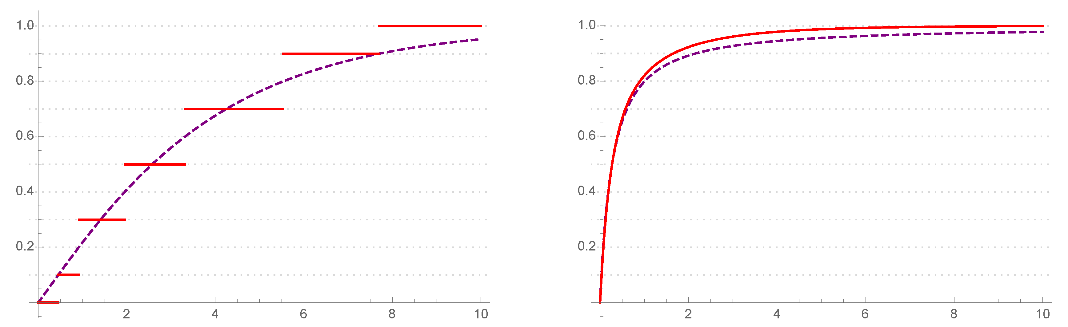
. Another possibility is to use the step function in Step 4d of our Algorithm 1; see also
Figure 1 for a graphical representation of the approximate step function and its corresponding hyperexponential distribution. Clearly, this new step function leads to
.
The error bound for the approximate ruin probability can be calculated afterwards through Theorem 1. An interesting question in this context is how many phases k for the approximate ladder height distribution suffice to guarantee an error bound for some predetermined . We answer this question in the next lemma.
Lemma 3. To achieve for some predetermined , the ladder height distribution must be approximated by a hyperexponential one with at least k phases, such thatwhere is the integer that is greater than or equal to x but smaller than . Proof. Observe that the error bound in Theorem 1 depends on the approximate hyperexponential distribution
, which means that one should first determine
and then calculate the error bound. However, when
, this translates to
. Therefore, the worst-case scenario for the bound is when
and consequently
. As a result, if we want to achieve
for all possible scenarios of
, we should solve the inequality
with respect to
. By substituting
, we calculate
In addition, the bound is asymptotically equal to
according to Remark 1. Consequently, it must also hold that
Finally, as the number of phases
k must be an integer, the smallest possible integer that satisfies at least one of the inequalities is the one described in Equation (
12). □
After this, we present our algorithm under the setting that we fix the desired accuracy for the approximation of the ruin probability .
| Algorithm 1. Spectral Approximation |
| Steps: |
Calculate the roots , using Equation ( 6). Find the spectral cdf of . Use Proposition 1 to calculate the spectral cdf of . Approximate by a hyperexponential distribution with k phases.
- (a)
Choose the accuracy of the ruin probability for a fixed . - (b)
Calculate k required to achieve this accuracy using Lemma 3 and set . - (c)
Define k quantiles such that , , , and . - (d)
Approximate the spectral cdf with the step function
- (e)
Find the ladder height distribution and calculate its Laplace transform .
Calculate the Laplace transform of the ruin probability as . Use simple fraction decomposition to determine positive real numbers , , , with , such that . Invert the previous Laplace transform to find , . The accuracy for is then , .
|
Remark 3. The decomposition of at Step 6 is guaranteed by Asmussen and Rolski (1992), who showed that the ruin probability in the Sparre Andersen model has a phase-type representation when the claim sizes are phase-type. Moreover, the particular hyperexponential representation of at Step 7 occurs because the poles of are exactly the roots of the polynomial function , where is the Kronecker delta. It is immediate from perturbation theory that has exactly k simple roots analytic in ϕ; see Baumgärtel (1985) for details. Remark 4. The above algorithm is an extension of the one developed for the Cramér–Lundberg model in Vatamidou et al. (2014), to which we refer for further details on technical implementation. 4. Asymptotic Approximation
In many cases, it is of importance to investigate the asymptotic behaviour of the ruin probability when the initial risk reserve tends to infinity. This question is particularly interesting in the case of heavy-tailed claim sizes. Towards this direction, when the claim sizes belong to the class of subexponential distributions
(
Teugels 1975), e.g., Pareto, Weibull, Lognormal, etc., the following asymptotic approximation is classical (see, e.g.,
Embrechts and Veraverbeke 1982):
Theorem 3. Suppose in the general Sparre Andersen model that the claim sizes and interclaim times have both finite means and , respectively, such that . If , then Note that the heavy-tail approximation
holds for any interclaim time distribution. However, further modifications have been attained in
Willmot (
1999), when the Laplace transform of the interclaim times is a rational function of the form (
5) with
and
belongs to the subclass of regularly varying distributions, i.e.,
,
, where
a slowly varying function and
,
. For example, the Pareto
distribution (see
Section 5.2.1) belongs to the class of regularly varying distributions with
,
and
, and its modified asymptotic approximation is then given by
which is smaller than
by a factor
that converges to 1 as
; see
Willmot (
1999) for details.
Clearly, the heavy-tail approximation admits a simple formula whenever the expectations of the interclaim times and claim sizes are finite; however, it has a drawback that occurs when the approximation is useful only for extremely large values of u.
In the next section, we compare the accuracy of the spectral approximation to the accuracy of the heavy tail one, i.e., . An interesting observation is that the spectral approximation converges faster to zero than any heavy-tailed distribution due to the exponential decay rate of the former. Thus, the heavy-tail approximation is expected to outperform the spectral approximation in the far tail, but for medium values, this new approximation can be very competitive.
5. Numerical Analysis
The goal of this section is to implement our algorithm in order to check the accuracy of the spectral approximation and the tightness of its accompanying bound, which is given in Theorem 1. To perform the numerical examples, we need to make a selection for the distribution K of the interclaim times as well as the claim size distribution .
5.1. Interclaims Times
We choose a hyperexponential distribution with two phases, i.e.,
, such that
. As
, it is evident that there exists only one positive and real root
to the generalised Lundberg equation of Equation (
6). Therefore, given also that
, the ladder height distribution takes the form
which is in accordance with
Li and Garrido (
2005).
5.2. Claim Sizes
For the claim sizes, we consider the Pareto distribution with shape parameter and scale parameter and the Weibull distribution with c and a positive shape and scale parameters, respectively.
5.2.1. Pareto
This distribution is c.m., as its ccdf
can be written as the LST of the Gamma distribution with shape and scale parameters
a and
b, respectively, i.e.,
The
nth moment of the Pareto distribution exists if and only if the shape parameter is greater than
n. As we are interested in comparing the spectral approximation to the asymptotic approximation of
Section 4, it is necessary to have a finite first moment for the claim sizes. Therefore, the shape parameter
a must be chosen to be greater than 1.
Using Proposition 1, we can easily verify that
5.2.2. Weibull
It can be verified that the ccdf
with fixed shape parameter
arises as a c.m. distribution (
Jewell 1982), where the mixing measure (measure of the spectral function)
S is given by
Similarly, we can find using Proposition 1 that
5.3. Numerical Results
The goal of this section is to implement our algorithm to check the accuracy of the spectral approximation and the tightness of its accompanying bound, which is given in Theorem 1.
For Pareto claim sizes, we choose , , , , and , and we obtain , and . For Weibull claim sizes, we choose , , , and , and we obtain , and . Note that we performed extensive numerical experiments for various combinations of parameters, but we chose to present only these two cases since the qualitative conclusions are comparable among all cases. Our experiments are illustrated below.
Impact of phases. It is intuitively true that the spectral approximation becomes more accurate as the number of phases increases. To test this hypothesis, we compare three different spectral approximations with number of phases 10, 30 and 100, respectively, with the exact value of the ruin probability (which we obtain through simulation). We display our results in
Table 1 only for Pareto claim sizes. The conclusion is that, indeed, a more accurate spectral approximation is achieved, as the number of phases increases for every fixed initial capital
u, which is in line with expectations.
Quality of the bound. A compelling question regarding the bound is if it is strict or pessimistic, i.e., how far it is from the true error of the spectral approximation. To answer this question, we first need to determine the accuracy
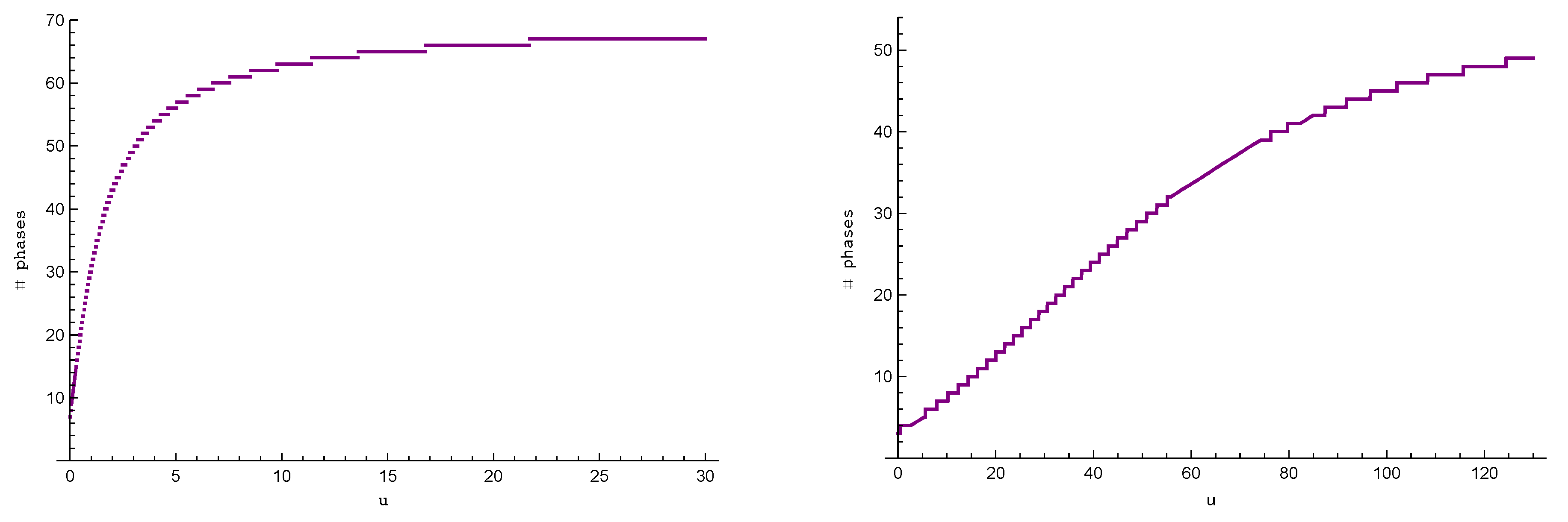
we would like to guarantee for the ruin probability. Using Lemma 3, we present, in
Figure 2, the number of phases required in order to guarantee
under Pareto
claim sizes and
under Weibull
claim sizes as a function of
u. For
, the required number of phases is equal to
in the Pareto case. Similarly, we find that
for
in the Weibull case. We generate the spectral approximations with 67 and 11 phases, respectively, and compare in
Figure 3 the true error (difference between simulation and spectral approximation) with the predicted error bound of Theorem 1 (green dotted line). The dashed cyan line in the left graph represents the worst-case scenario for the bound that was used in the proof of Lemma 3 to calculate the optimal number of phases to guarantee an error of at most
up to
.
As we can observe in
Figure 3, the true error is significantly smaller than the predicted error bound for small values of
u, under Pareto
claim sizes. This may be because, for small values of
u, a smaller number of phases
k is enough to guarantee
; see also
Figure 2. Afterwards, the true error increases to the error bound by reaching its maximum value close to
, and then drops to zero as
, whereas the predicted bound remains constant. A similar behaviour is recognised under Weibull
claim sizes, where now the true error is close to the predicted error bound for small values of
u, as
is already a small number itself.
Finally, notice that the predicted error bound is almost 4 times smaller than
in the Pareto case. This happens because
could be a lot smaller than
; see also
Figure 1 where
. However, most importantly, the true error is close to the predicted bound, and thus we can say that Lemma 3 provides a good proxy for the necessary number of phases
k to achieve it.
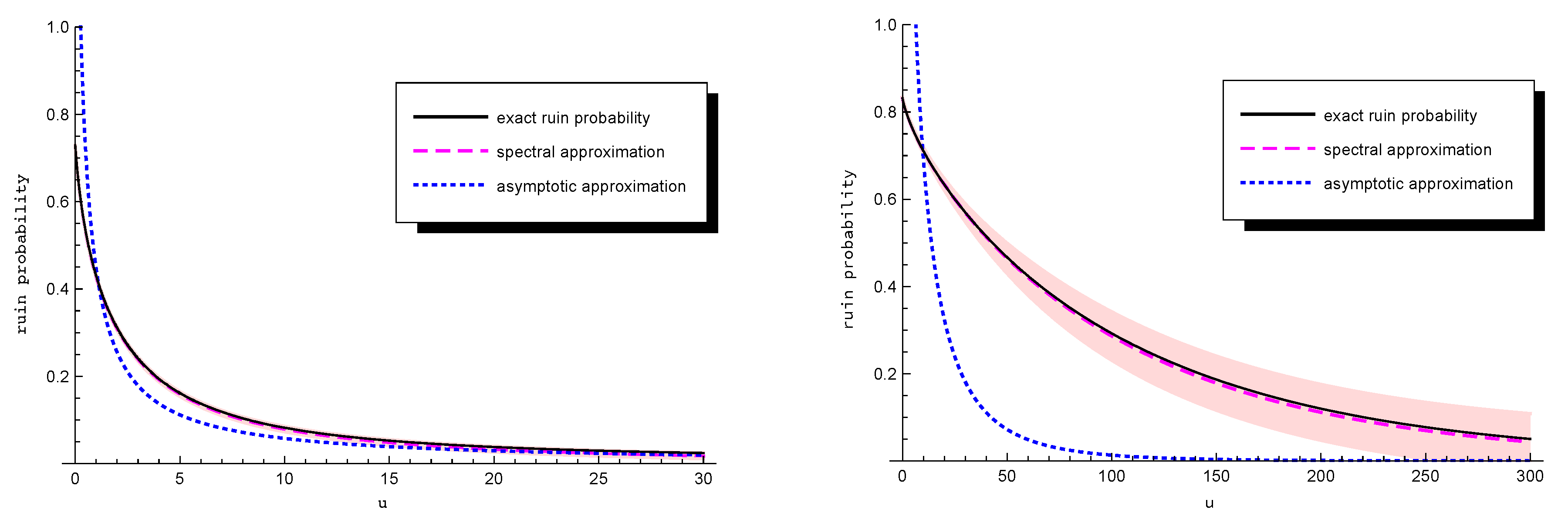
Comparison between spectral and heavy-tail approximations. As we pointed out in
Section 4, the spectral approximation is expected to underestimate both the exact ruin probability and the asymptotic approximation
in Theorem 3 for large
u, due to its exponential decay rate. It is of interest to see the magnitude of
u for which the asymptotic approximation outperforms the spectral approximation.
We select the spectral approximations with
phases for Pareto
claim sizes and
phases for Weibull
claim sizes, as in the previous experiment, and present the distributions in a graph. The pink shadow in
Figure 4 enfolding the spectral approximation represents its bound. We observe that for small values of
u, the spectral approximation is more accurate than the heavy-tail approximation, where the second provides a rough estimate of the ruin probability. On the other hand, the heavy-tail approximation is slightly more accurate than the spectral approximation in the tail, i.e., for
, under Pareto claim sizes. However, for the Weibull case, we observe that, even for values of
u around 300, the spectral approximation still outperforms the heavy-tail approximation.
6. Conclusions
In this paper, we considered the ruin probability of the Sparre Andersen model with heavy-tailed claim sizes and interclaim times with rational Laplace transform. Using the geometric random sum representation, we developed an explicit bound and also constructed a spectral approximation by approximating the c.m. ladder height distribution with a hyperexponential one. Our spectral approximation algorithm advances on the algorithm established in
Vatamidou et al. (
2014) in various aspects. We provide below a summary of our conclusions both for the spectral approximation and the bound.
When comparing with the technique proposed in
Vatamidou et al. (
2014), the strategic selection of the quantiles in Step 4d reduces the number of phases to almost a half, to guarantee a certain accuracy for the ladder height distribution.
As the bound depends on the initial capital, we were able to focus on one area and optimise the required number of phases to achieve a desired accuracy, e.g., we would need 110 phases for and 132 phases for to guarantee accuracy of at most in our example.
The step function is constructed to guarantee , but in most applications is a lot smaller than . Thus, the use of in the bound makes it tighter.
To sum up, the spectral approximation is highly accurate for all values of u as opposed to the heavy-tail approximation, which fails to provide a good fit for small values. Moreover, it is accompanied by a rather tight bound.
Finally, note that the results of this paper are also valid for the risk model with two-sided jumps, i.e.,
where
u,
c and
are defined as before, whereas
and
are independent Poisson processes with intensities
and
, respectively; see, e.g.,
Albrecher et al. (
2010). In addition, the sequence
of i.i.d. r.v.’s, independent of
,
and
, and having the common d.f.
that belongs to the class of distributions with rational Laplace transform, are the sizes of premium payments. The positive security loading condition in this model becomes
.
Let
be the time when the
nth claim occurs with
. As ruin occurs only at the epochs when claims occur, we define the discrete time process
, where
and
, which denotes the surplus immediately after the
nth claim, i.e.,
where
with
. Equation (
14) corresponds to the discrete-time embedded process of the Sparre Andersen risk model (
1), and the counting process
denotes the number of claims up to time
t with the modified interclaim times
. Clearly,
where
is the Laplace transform of the premium payments; see
Dong and Liu (
2013). Let now
and
. Obviously,
.


