The OFR Financial Stress Index

Office of Financial Research, 717 14th St NW, Washington, DC 20005, USA
Risks 2019, 7(1), 25; https://doi.org/10.3390/risks7010025
Submission received: 28 January 2019
/
Revised: 21 February 2019
/
Accepted: 21 February 2019
/
Published: 26 February 2019
(This article belongs to the Special Issue Financial Risks and Regulation)
Abstract
:We introduce a financial stress index that was developed by the Office of Financial Research (OFR FSI) and detail its purpose, construction, interpretation, and use in financial market monitoring. The index employs a novel and flexible methodology using daily data from global financial markets. Analysis for the 2000–2018 time period is presented. Using a logistic regression framework and dates of government intervention in the financial system as a proxy for stress events, we found that the OFR FSI performs well in identifying systemic financial stress. In addition, we find that the OFR FSI leads the Chicago Fed National Activity Index in a Granger causality analysis, suggesting that increases in financial stress help predict decreases in economic activity.
1. Introduction
The history of financial markets demonstrates that financial crises are often followed by large and persistent reductions in real economic activity. The 2007–2009 global financial crisis was a devastating illustration of this. The crisis also made it clear that the modern financial system is global and highly interconnected, and that these interconnections can potentially act as conduits to propagate idiosyncratic shocks across the system in a contagion effect. Because of the potential for negative spillover of financial stress events onto the real economy, accurately measuring financial stress is important to policymakers, who require clear and timely signals of market strains to develop appropriate policy responses to address these events.
Unlike other indicators in the economy such as stock prices or the unemployment rates, financial stress is not directly observed and must instead be estimated. This paper introduces a financial stress index (FSI) developed by the Office of Financial Research (OFR). The OFR FSI is a daily, market-based snapshot of systemic financial stress in global financial markets available to policymakers at the Financial Stability Oversight Council, its member agencies, the financial industry, Congress, and the public. The index distills information embedded in more than 30 indicators into a summary measure of systemic financial stress. It can be decomposed into five categories of indicators or three regions, allowing users to drill down into the drivers of financial stress.1
The Dodd-Frank Wall Street Reform and Consumer Protection Act of 2010 mandates the OFR to develop and maintain metrics and reporting systems for risks to financial stability. The law also gives the OFR the responsibility to monitor, investigate, and report on changes in systemwide risk levels and patterns. The OFR FSI complements other financial stability monitoring efforts at the OFR, particularly the Financial System Vulnerabilities Monitor, or FSVM. While the FSVM is intended to provide advanced warning of potential problems, the FSI measures the severity and nature of stress as it occurs. Vulnerabilities can build during periods of low stress. For example, historically high asset valuations can be viewed as a financial stability vulnerability because they suggest that investors have complacent attitudes toward risk. During a time of high asset valuations, stress is likely to be low. However, a sudden and large decline in asset valuations can indicate stress resulting from a shock in investor preferences or risk appetite. Stress and vulnerabilities should therefore be measured separately.
The OFR FSI is distinguished from other FSIs2 by its global scope, daily frequency, dynamic weighting scheme, transparent and methodical construction, and its ability to be decomposed into indicator categories and regions. Unlike some other FSIs, whose entire time series are re-estimated each time they are updated, the OFR FSI respects the arrow of time. The OFR FSI’s value on a given day depends only on information available that day and, once estimated, its value does not change. The OFR FSI’s methodology also accommodates input indicators of differing historical timespans. Importantly, as financial markets evolve, indicators that cease to reflect market participants’ views about financial stress can be removed and replaced with more appropriate indicators.
The value of the OFR FSI on a given date is proportional to the weighted average of the marginal contributions to financial stress of its constituent indicators. The marginal contribution of an individual indicator to financial stress is its signed standardized value (its value relative to its historical mean, divided by its standard deviation, and signed so that increases in the indicator correspond to increases in financial stress). The weights and the signs of indicators’ stress contributions are determined using a dynamic factor model with a single latent factor, which essentially corresponds to the first principal component from a principal component analysis. The index is positive if the (weighted) average stress contribution of the indicators is positive. The index is zero if the average is zero, and negative if the average is negative.
The OFR FSI is constructed in two steps. First, a set of indicators that reflect financial stress is assembled. We define financial stress as disruptions in the typical functioning of financial markets. Symptoms of financial stress are informed by both theory and practice, and include: uncertainty about the fundamental value of financial assets or the behavior of investors; increased asymmetric information; and a decreased willingness to hold risky or illiquid assets (Hakkio and Keeton 2009). Indicators for the index must reflect one or more of these symptoms of stress in a timely manner. In addition, we seek broad and roughly balanced coverage across asset classes and global regions, including representation from U.S.-domiciled financial markets, markets from other advanced economies such as the eurozone and Japan, and emerging markets. The set of indicators is quantitatively screened, and redundant indicators are eliminated. The result of this process is a set of over 30 global financial market indicators, such as implied volatility indexes, yield spreads, valuation measures, and interest rates that are available with varying historical timespans at a daily frequency from publicly available sources.
The second step in the construction of the OFR FSI on a given date is aggregating the set of indicators into a composite index. First, the component indicators are converted to a common unit by taking each indicator, subtracting its mean up until that date, and dividing by its standard deviation. The index is intended to capture systemic financial stress, which occurs when exogenous shocks or contagion effects occur in multiple markets simultaneously. We estimate this simultaneous co-movement using a dynamic factor model with a single latent factor that essentially corresponds to the first principal component. Unlike classical principal component techniques, however, the factor model accommodates indicators of differing historical time spans. This aspect of the methodology means that the set of indicators in the index can change in the future as the financial system evolves. When the next date is estimated, the indicators are re-standardized, and the factor model is re-estimated. As such, the OFR FSI’s value depends only on information up until the date on which it is estimated. Unlike some other FSIs, the OFR FSI’s past values are not re-estimated each time the model is estimated.
The first-order conditions from the procedure can be used to decompose the index into the marginal contributions of individual indicators to stress. These individual contributions are aggregated into sub-components reflecting the type of indicator. The indicator categories are credit spreads, equity valuation, funding, safe assets, and volatility. These indicator categories are useful for monitoring the drivers of stress. Similarly, the index can be decomposed by region into contributions from U.S. markets, other advanced economies, and emerging markets.
After detailing the construction of the index, we present a summary of its behavior over the 2000–2018 time period. We then discuss specific examples of market monitoring using the OFR FSI. The use cases include the 2007–2009 global financial crisis, the subsequent European sovereign debt crisis, and the recent events of 2018. The index and its decomposition into indicator categories and regions allow us to drill down into the drivers of systemic financial stress, cutting through the clutter of market chatter. Decomposition of the index shows which types of indicators are telegraphing market participants’ views of stress. If indicator categories or region categories move together, we get some evidence of a systemic event.
A natural question is whether an FSI actually measures the latent indicator of financial stress. In Section 5, we discuss the empirical properties of the OFR FSI. Using dates of significant government intervention in financial markets as a proxy for financial stress events, we use logistic regression to show that the OFR FSI identifies financial stress periods well and is thus fit for its purpose. We then consider the relationship between financial stress and economic activity. Using the Chicago Fed National Activity Index as a proxy for real economic activity, we use Granger non-causality analysis and conclude that high levels of financial stress help predict decreases in economic activity.
This paper proceeds as follows. The next section provides background on financial stress and financial stress indexes, and distinguishes them from systemic risk indicators. Section 3 describes the construction and interpretation of the OFR FSI. Section 4 illustrates the use of the OFR FSI in OFR monitoring efforts. Section 5 describes empirical properties of the index. Section 6 concludes.
2. Systemic Financial Stress and Financial Stress Indexes
The global financial crisis of 2007–2009 showed that stress events in the financial sector can have severe adverse consequences for real economic activity in terms of output, employment, and welfare. It also underscored the need for policymakers to have accurate and timely signals of financial stress to respond appropriately to mitigate the impact of financial stress events. Since the crisis, policymakers and researchers have become more keenly aware of, and interested in, systemic risk and financial stress.
Financial stress is an unobserved variable in the economy. Several attempts have been made to define and measure it (see Kliesen et al. (2012) and Hatzius et al. (2010) for surveys). Some researchers define financial stress as being directly related to financial market functioning (Carlson et al. 2012; Sandahl et al. 2011). Others define stress indirectly as “systemic risk which has materialized” (Louzis and Vouldis 2013) or as the product of the interactions between vulnerabilities in markets and shocks (Grimaldi 2010, 2011). Although there is yet to be a consensus on what specifically constitutes financial stress or a financial stress event, there are common elements among these notions of stress, and this motivates the following definition: financial stress refers to disruptions to the normal functioning of financial markets. The definition is purposely broad, as financial stress can manifest in different ways, and no two stress events are exactly the same. Furthermore, note that financial stress thus defined is not synonymous with materialized systemic risk. Financial stress events can be reflected in some markets but not in others. However, extremely high levels of financial stress likely correlate with truly systemic financial stress events.
Although stress events differ in composition, there are several common economic characteristics of financial stress. Hakkio and Keeton 2009 survey the academic literature and summarize the symptoms of financial stress. According to their framework, financial stress is characterized by the coincident manifestation of one or more of the following:
- Increased uncertainty about the fundamental value of assets or the behavior of investors. Volatility may rise when increased uncertainty causes investors to react more strongly to new information. Increased uncertainty can be measured by implied or realized volatility.
- Increased asymmetry of information. Asymmetric information can worsen during a stress event if variation in true quality of borrowers or assets increases, or if information is deemed less reliable. Information asymmetries can lead to problems of moral hazard and adverse selection, and to increased borrowing costs and decreased asset prices. Asymmetric information can be measured by increases in credit or funding spreads or decreases in risky asset valuations.
- Decreased willingness to hold risky assets. Investors that change their preferences or risk appetite may demand more compensation for holding risky assets. This change may lead to price decreases of risky assets and price increases of safe assets. The change can be measured by decreases in risky asset valuations or increases in safe asset valuations.
- Decreased willingness to hold illiquid assets. Investors may become reluctant to hold illiquid assets if demand for liquidity increases in anticipation of unexpected needs for cash. This change may be due to rising volatility, or a perceived deterioration in asset liquidity. The change can be measured by increases in funding spreads.
These symptoms of financial stress are not directly observed in financial market indicators. Instead, financial market indicators that reflect one or more of the above symptoms of stress are collected to monitor stress. A financial stress index is a univariate time series that aggregates the information in these indicators and isolates and measures the level of financial stress.
Financial stress indexes are similar to financial conditions indexes (FCIs). Like FSIs, FCIs combine information from many financial indicators to create a univariate time series that represents conditions in the financial system. The main difference between FSIs and FCIs is in their objectives. The objective of FCIs is to focus on the link between the financial sector and the real economy. Conversely, FSIs are concerned with distress or instability in the financial system without explicit regard for how such distress may manifest in the real economy.
Another principal difference between FSIs and FCIs is in the set of indicators used in their construction. FSIs are generally constructed with market price-based measures. FCIs, on the other hand, are constructed with price-based measures and also include other market characteristics such as flows, trading volume, and stock measures. In practice, there is often considerable overlap between FSIs and FCIs in the sets of indicators included and the construction techniques used. Consequently, there is often considerable overlap in the time series properties of FSIs and FCIs.
A number of FSIs and FCIs have been developed over the past decade or so in the aftermath of the 2007–2009 global financial crisis. Here we only mention a few, and we refer the reader to Kliesen et al. (2012) and Hatzius et al. (2010) for more detailed surveys of various FSIs and FCIs. One of the first FSIs was developed by Illing and Liu (2006) for the Canadian financial market. They aggregate several indicators based on the specification that performs best in crisis times, where such times are identified from surveying policymakers at the Bank of Canada. Notable FSIs that focus on the U.S. financial system have been developed by two regional banks in the Federal Reserve System—the Kansas City Fed Stress Index (Hakkio and Keeton 2009) and the St. Louis Fed Stress Index (Kliesen and Smith 2010). Both FSIs aggregate indicators based on principal components, the notion being that the indicators are picked such that financial stress is manifest when they co-move. Carlson et al. (2012) at the Board of Governors of the Federal Reserve also develop a U.S.-based FSI. Some researchers, particularly in the eurozone, have developed individual FSIs to monitor financial stress in particular countries. Examples include Cardarelli et al. (2011), who created FSIs for 17 advanced economies, Lo Duca and Peltonen (2011), who produced FSIs for 10 advanced and 18 emerging economies, and Duprey et al. (2017), who constructed FSIs for 27 EU member countries and applied a Markov-switching model to endogenously determine high financial stress periods (see also Duprey and Klaus (2017)). Others have constructed FSIs to examine the relationship between financial stress and macroeconomic variables (Apostolakis and Papadopoulos 2019) or exchange rates (Adam et al. 2018). Vasicek et al. (2017) show that FSIs are difficult to forecast out-of-sample.
Many FCIs have also been developed. Notable examples include the Bloomberg FCI (Rosenberg 2009), which is based on simple arithmetic averaging, and Hatzius et al. (2010) and the Chicago Fed National FCI (Brave and Butters 2011), which both use a dynamic factor model methodology.
Generally, FSIs and FCIs have been constructed in two broad steps. First, a set of observable financial market indicators that reflect stress is assembled. For FSIs, the indicators are nearly universally market-determined prices, reflecting the assumption that markets are the best and quickest aggregators of available information. Common types of indicators included are measures of volatility, credit spreads, funding spreads, and interest rates. After a set of indicators is determined, the second step is to process and aggregate the information contained in these indicators into a single summary measure of stress. Several methods of aggregation are used in the literature. The most common ways are a simple average (Lo Duca and Peltonen 2011), simple averages of sub-indexes (Rosenberg 2009), or by using statistical techniques like principal components analysis (PCA) (Kliesen and Smith 2010; Hakkio and Keeton 2009) or dynamic factor models (Hatzius et al. 2010; Brave and Butters 2011). Some authors take other approaches, such as methods inspired by portfolio theory (Hollo et al. 2012) or logistic regression models based on a pre-defined stress event indicator (Nelson and Perli 2007; Carlson et al. 2012).
The post-crisis environment has also been fertile ground for development of systemic risk indicators, or SRIs. SRIs measure vulnerabilities rather than stress. Examples of these include the conditional value at risk (CoVaR) (Adrian and Brunnermeier 2016), the distressed insurance premium (DIP) (Huang et al. 2012), and the systemic expected shortfall (SES) (Acharya et al. 2017). Like financial stress, systemic risk has no universally accepted definition. Given that the financial system is large, complex, and constantly evolving, a diverse set of approaches and measures is needed to study systemic risk. SRIs such as CoVaR, DIP, SES, and most of the others outlined in the first OFR working paper (Bisias et al. 2012), tend to be institution-specific estimates of the effects of low-probability but consequential, or “tail,” market events. Bisias et al. (2012) develops a taxonomy of SRIs, classifying them by focus into macroprudential or microprudential measures and by horizon with respect to risk realization, as contemporaneous or ex-ante measures. As that paper demonstrates, most SRIs are microprudential measures focusing on effects conditional on an event relating to a financial institution. Such measures can be either contemporaneous to risk manifestation or could possibly give early warning signals. In contrast, an FSI is a market-based, macroprudential measure relaying an unconditional, contemporaneous view of market functioning. In other words, an FSI indicates what the state of the financial system is, and an SRI expresses what happens if the state of the financial system contains a specific stress event pertaining to that SRI.
3. Construction and Interpretation of the OFR FSI
The OFR FSI aims to provide a real-time summary measure of the level of financial stress by aggregating the information embedded in a number of market indicators related to stress. Here we detail the indicators included in the index and the way in which we combine them.
3.1. Indicator Selection
The OFR FSI has a transparent and methodical construction. The construction has two steps: indicator selection and indicator aggregation. Indicator selection begins with a survey of the literature and financial market landscape for indicators that reflect one or more of the symptoms of financial stress outlined in the previous section of this paper. After considering the symptoms of stress, we created five distinct indicator categories: credit, equity valuation, funding, safe assets, and volatility. Definitions of these categories appear in Table 1. While the OFR has a statutory mandate to monitor U.S. financial stability, it is important to recognize that stress from foreign markets can migrate to U.S. domestic markets. Accordingly, we consider three regions for classifying indicators: U.S.-centric, other advanced economies (such as the eurozone and Japan), and emerging markets. We require our set of indicators to have broad coverage across major asset classes, the five indicator categories, and the three regions. Moreover, we require each indicator to be—or be directly related to—a market-determined price.
Finally, we combine the qualitative factors with a quantitative test for redundant information. Taking advantage of the fact that the recent history in financial markets contains both a crisis period and periods of tranquility, we use a rolling 500-day pairwise correlation analysis to determine if two indicators substantially produce the same information during both volatile and tranquil periods. If this correlation is consistently high (greater than 0.8 in magnitude) through both the crisis period and bull markets, we consider them to be producing the same information. In the absence of a compelling reason to keep such an indicator in the index, such as for balance across indicator categories, we eliminate such an indicator from the set.
Appendix A contains information about our resulting set of indicators, including source, time span of data, indicator category, economy classification, transformation of the raw data before the aggregation step (to ensure approximate long-run stationarity), and basic summary statistics. All indicators in our set are available at a daily frequency, though this is not a strict requirement for inclusion because the indicator aggregation methodology (see next section) can accommodate indicators of different frequencies, such as weekly or monthly.
3.2. Indicator Aggregation
The 33 indicators used to construct the OFR FSI are chosen to reflect one or more symptoms of financial stress. We assume that financial stress manifests if and when the indicators move together. That is, the extent of the simultaneous co-movement in the indicators reflects systemic financial stress. This suggests that we use the first principal component from a principal components analysis.
We also want to account for relationships among indicators changing over time as the financial system evolves, which suggests a dynamic approach. The financial system may evolve to the point where certain indicators are no longer appropriate for measuring symptoms of financial stress and should be removed and possibly replaced. This is a particularly important aspect of the construction because as the financial system evolves, the set of indicators through which financial stress is manifest can change. For example, currently our set of indicators contains several measures related to the London Interbank Offered Rate (LIBOR) in its funding indicator category. Because of the attempted manipulation of LIBOR during the financial crisis and other problems, work is underway at the OFR and throughout the public and private sectors to develop a LIBOR replacement (ARRC 2017). If such a replacement proves successful and funding market strains are reflected through the new indicator, we will substitute it for LIBOR in the index.
Indicator composition may also change in the future for other reasons. For example, the rise of China as an important financial market over the past decade or so may merit the addition of Chinese indicators that have a sufficient time series and data quality. We may in the future decide that other markets, such as real estate, are worth including in the index, provided we can achieve balance across regions. These and practical data availability considerations suggest the need to accommodate unbalanced panels in our analysis.
Finally, to be useful in real time, a stress measurement on a given date should be measurable with respect to known information on that date. Historical measurements of stress should not depend on information or events that occurred subsequently. All these factors motivate the following approach and estimation method.
We estimate the degree of simultaneous co-movement using a dynamic factor model with a single latent factor, a generalization of classical principal components analysis or PCA. The vector of weights on the indicators from the model shows the direction of highest co-movement or correlation in the data. The vector of weights can be viewed as the single best summary of the correlations in the data. Unlike other PCA-based FSIs, we estimate this weights vector each time the index is calculated, using information available through that date and not information from subsequent dates. Past values of the index are not recomputed. Finally, as in Hatzius et al. (2010), the unbalanced structure of our panel dataset is accommodated by estimating the dynamic factor model using an iterative least squares technique rather than the classical singular value decomposition.
Suppose we want to calculate the OFR FSI on a given date . Let denote the matrix of the data from the indicators in the index through date , transformed according to Appendix A, and standardized to have zero mean and unit standard deviation. An indicator is eligible for inclusion on date if its historical time series goes back at least 500 trading days, which is approximately two years. We consider the following decomposition of the data:
where is the unobserved factor common across the indicators, is the unobserved loading of indicator on this factor, and is the residual variation in , which is assumed to be uncorrelated across the indicators. Note that , , , and all depend on the fixed time , but for ease of exposition, we have dropped the reference to .
We want to estimate the vector of indicator weights and the vector of the common factor. Solutions of (1) are unique up to a constant, and so without loss of generality we impose the constraint that the vector has norm one and points in the direction most resembling the expected signs on the indicators (see Appendix A). To estimate we follow the approach in Hatzius et al. using least squares (see also Bai and Ng (2008) and Stock and Watson (2002, 2006, 2010)). That is, and solve
where we only sum over non-null observations of the indicators. This optimization problem is solved using iterative methods.3 (If the matrix represented a balanced panel, the solution would be given by classical principal components, i.e., by computing the eigenvectors of the sample correlation matrix.) The value of the OFR FSI on date is then given by , the estimated factor evaluated at time . The decomposition of the OFR FSI into indicator-level contributions and indicator categories follows from the first order condition of (2), namely that
where is the Moore-Penrose pseudoinverse of , is the -th column of representing the time series of the -th indicator, and we have used our assumption that the norm of is one. Thus, the OFR FSI decomposes as a sum of contributions over the set of indicators in the index. By summing contributions of indicators in each indicator category, we obtain the subtotals for the credit, equity valuation, funding, safe assets, and volatility indicator categories. Similarly, by summing contributions of indicators in each region, we obtain the subtotals for the United States, other advanced economies, and emerging markets. Note that indicators that are assigned multiple regions have their contributions evenly divided among the assigned regions.
3.3. The Index and Its Interpretation
Table 2 provides a decomposition of the OFR FSI on 31 December 2018. The 33 indicators used in the index are listed in their respective indicator categories.4 The other columns in the table provide each indicator’s weight in the loading vector (Coef.) as determined by the dynamic factor model; the value of the indicator on 31 December 2018, standardized with respect to its history up until that time (Data); and the contribution of the indicator to systemic financial stress (Contr.), which is the product of these values. The units of an indicator’s standardized value are in the number of standard deviations, and thus, each indicator’s weight in the loading vector is naturally interpreted as a sensitivity, that is, as the incremental change in the OFR FSI associated to a one standard deviation increase in the indicator. For example, the coefficient on the Chicago Board Options Exchange Volatility Index, or VIX, on 31 December 2018 was 0.254, and therefore, an increase of one standard deviation in VIX on that date was associated with a 0.254 incremental increase in financial stress, all else being equal. The relationships among the coefficients on the indicators also have important implications about indicators’ relative contributions to stress. The coefficient on 31 December 2018 on the 10-year U.S. Treasury note, for example, was −0.105, which in absolute terms is about 40 percent of the coefficient on VIX. This implies that, all else being equal, a one standard deviation decrease in the 10-year Treasury note yield5 had about 40 percent of the effect on systemic financial stress as a one standard deviation move in the VIX.
The contribution column reports the product of each indicator’s weight in the loading vector and its standardized data on 31 December 2018. This value is unitless and is the marginal contribution of the indicator to financial stress. Summing the marginal contributions of the indicators in a given indicator category gives the marginal contribution to financial stress of the category on that date. Similar summing over all the marginal contributions of the indicator categories gives the value of the OFR FSI on that date. An FSI value of zero implies that either all indicators have exactly zero marginal contributions to financial stress or that positive marginal contributions are exactly offset by negative marginal contributions to stress. A necessary but not sufficient condition for this to occur is that each indicator has exactly average performance on the date of the FSI. Positive (negative) values of the FSI arise when the positive (negative) marginal contributions outweigh the negative (positive) marginal contributions. For example, the standardized value of VIX on 31 December 2018 was above average, at 0.790, implying a contribution to financial stress of 0.201 on that date. The contribution to stress for the volatility indicator category, equal to −0.326, is computed by summing the marginal contributions of the nine indicators included in the volatility indicator category. Finally, the value of the OFR FSI is computed by summing the marginal contributions of the various risk dimensions, returning 0.268. Examining the marginal contributions of the indicators and indicator categories provides insight on what was driving financial stress on a given date. On 31 December 2018, above average stress in the equity valuation and credit subcategories was balanced by below average stress in the volatility and funding subcategories.
The information in Table 2 facilitates another interpretation of the OFR FSI: the value of the OFR FSI on a given date is proportional to the weighted average of the standardized values of its constituent indicators. This can be easily seen by examining the Wgt. and Data* columns in Table 2. The Wgt. column is simply the absolute value of the Coef. column, the column of indicator weights from the dynamic factor model. The Data* column is just the standardized value of the indicator on that date, signed to reflect that increases in the indicator correspond to increases in financial stress. The value of the index is then the weighted average, using the weights in Wgt, of these signed standardized values in Data*. The index is positive if the (weighted) average standardized values of the indicators is positive, is zero if this average is zero, and is negative if the average is negative.
Additional interpretation of the OFR FSI can be gained by rewriting it on a given date as (see (3))
where is the standardized data from date and cos is the angle in Euclidean space between the first loading vector and the standardized data vector . This decomposition shows that the FSI is determined by the size of the standardized data vector and the angle of with the first loading vector . For a fixed angle between and , the farther the indicators are from their average, the larger the composite size of the data will be and consequently the larger the FSI will be. Conversely, for a given deviation of the indicators from their respective means, i.e., for a given , systemic financial stress as reflected in the FSI is maximized when the angle between and is zero, i.e., when is a positive multiple of . That is, given a fixed aggregate deviation of the indicators from their means, the FSI is maximized when the relative relationships reflected in the vector across all of the indicators the indicators are maintained. The vector is interpreted as the direction of maximal systemic financial stress. By providing the direction of maximized financial stress, the first loading vector on a given day provides a multidimensional measure of vulnerability in financial markets.
4. Use of the OFR FSI in Market Monitoring
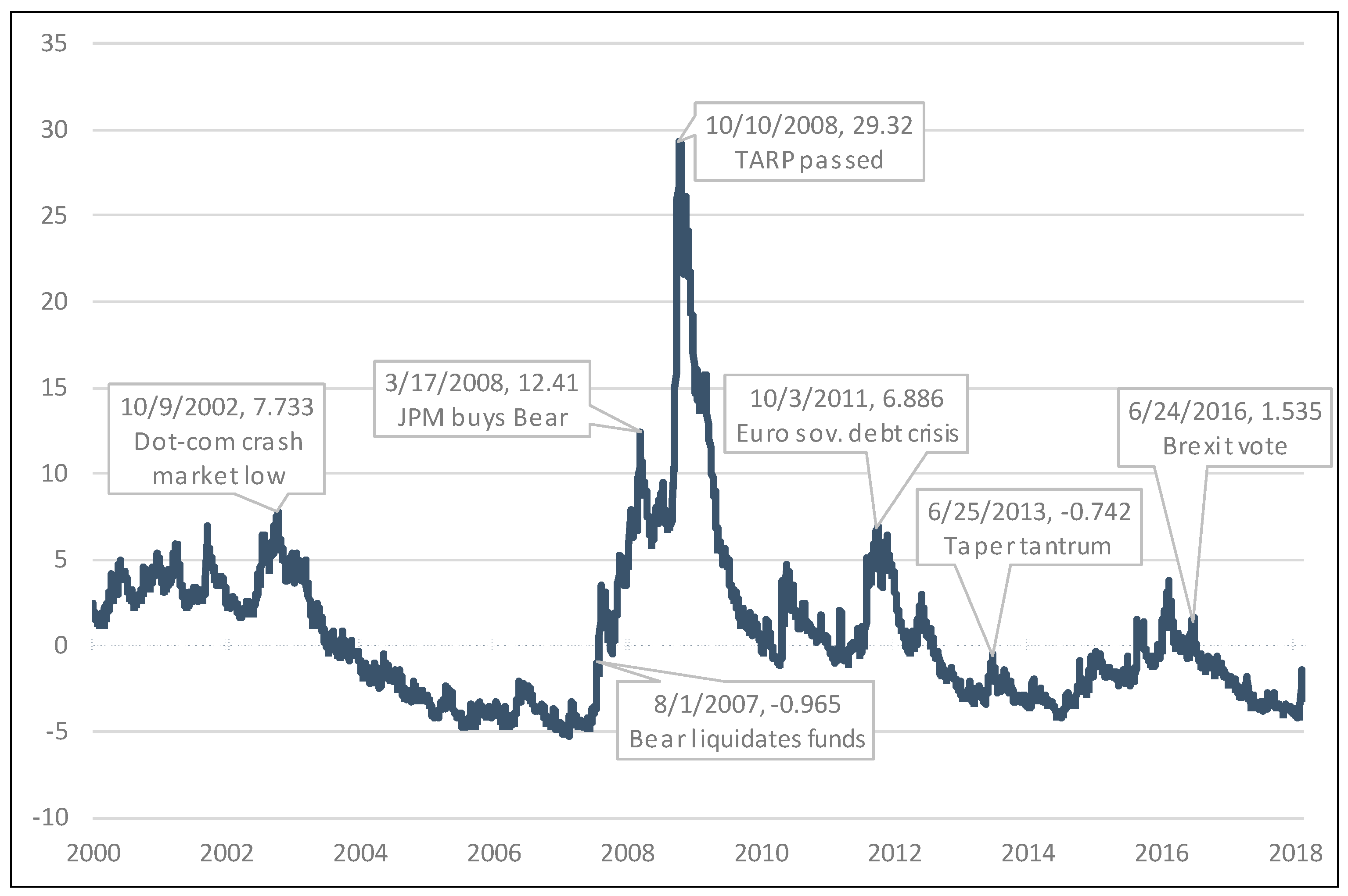
The OFR FSI is plotted from its inception in January 2000 through the end of December 2018 in Figure 1. Several dates of interest are labeled.
The OFR FSI was positive during the bust of the dot-com bubble, before declining into negative territory during the bull market of the mid-2000s. The index increased precipitously in mid-2007 during the beginnings of the global financial crisis; Figure 1 notes the date Bear Stearns liquidated two hedge funds with exposures to subprime mortgages. The OFR FSI continued to increase through March 2008 when JPMorgan Chase & Co. agreed to buy Bear Stearns. Throughout the summer of 2008, the index remained high, and it rose in the fall when Lehman Brothers sought bankruptcy protection. The OFR FSI hit its apex in October and November 2008 after Congress approved the Troubled Asset Relief Program (TARP). The index eased but remained relatively high through 2009. It increased again during the European sovereign debt crisis of 2010 and 2011. Since then, the OFR FSI has generally declined, with some of its lowest levels since before the crisis occurring during 2018.
Figure 2 shows the index and its decomposition into indicator categories during the 2007–2009 global financial crisis. The OFR FSI started the period at around negative 5, increased steadily through mid-2008 to about 7, and then jumped in the second half of 2007 as the crisis took hold, before declining but still remaining positive during the first half of 2009. Figure 2 shows that stress in each of the five categories was below average until mid-2007, when stress spiked mainly in volatility and funding subcomponents. Stress continued on an upward trend as the credit indicators increased and volatility and funding indicators remained high. Stress from the credit, volatility, funding, and equity valuation categories simultaneously spiked in the fall of 2008, propelling the FSI to its all-time high and illustrating the contagion effect during the global financial crisis.
4.1. The European Sovereign Debt Crisis
By 2012, the European sovereign debt crisis was well underway. Bailouts and other government support throughout the global financial crisis of 2007–2009 led to balance sheet strains for many sovereigns, particularly in Europe where some sovereigns were already heavily indebted. Concern over a possible Greek sovereign debt default continued to build in 2009 and 2010, and eventually spread to Portugal, Ireland, and Spain. In late 2010 and early 2011, the EU and International Monetary Fund (IMF) agreed to bailout packages for Greece, Ireland, and Portugal.
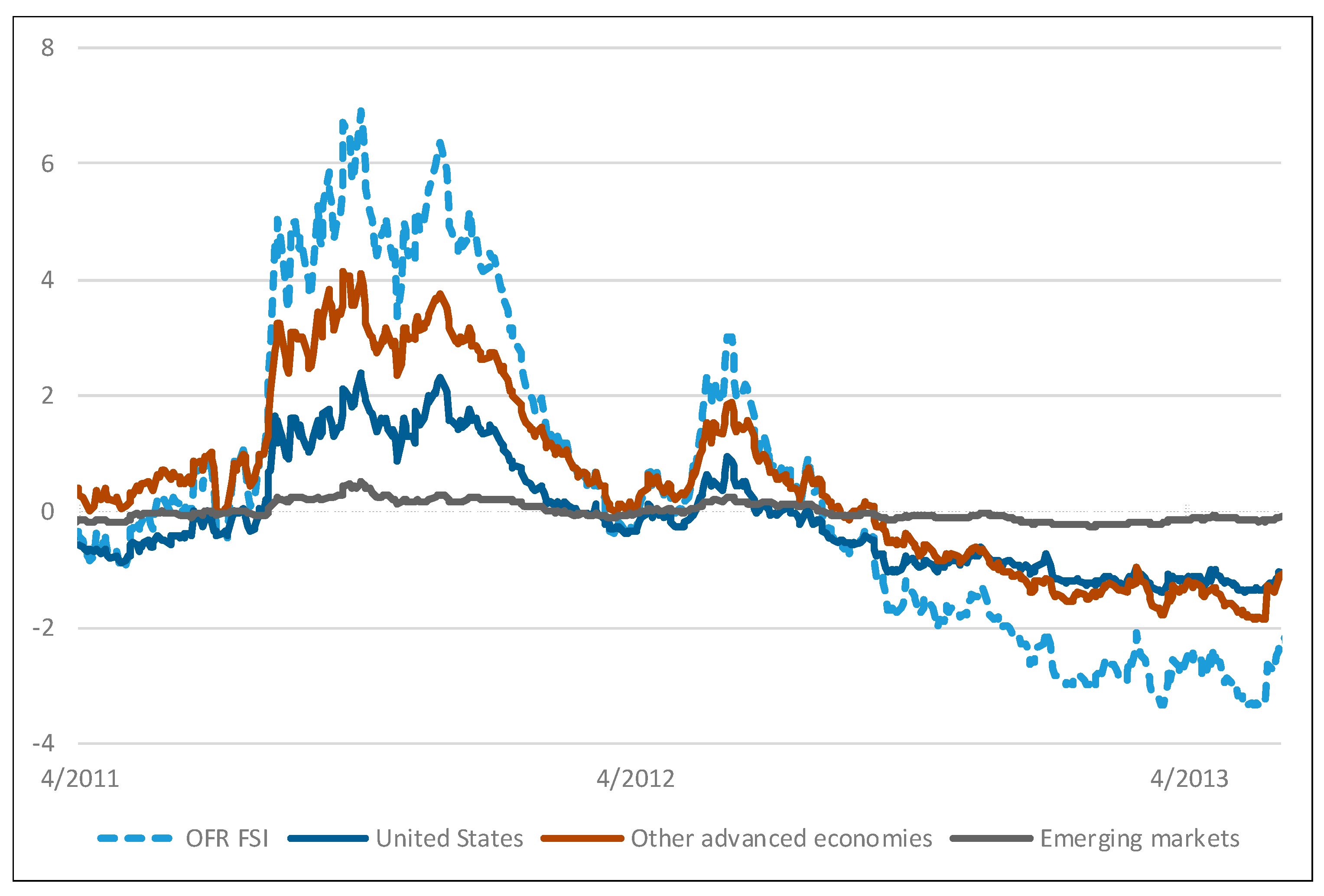
Figure 3 depicts the OFR FSI and its indicator categories from April 2011 through May 2013. During late spring and early summer in 2011, market participants became concerned that Greece might become the first country to leave the eurozone. Stress increased slowly during this period from normal levels, except for a short-lived decline in July when the eurozone agreed to a Greece bailout package of over 100 EUR billion to contain potential contagion. However, stress spiked dramatically in August as the result of two events: Standard and Poor’s downgraded the credit rating of U.S. sovereign debt for the first time in history, and the European Commission expressed concerns that the sovereign debt crisis was spreading. Italian and Spanish sovereign bond yields rapidly rose as fears of contagion manifested. This increase in stress appeared in all indicator categories of the OFR FSI, particularly the volatility, credit, and funding categories. Figure 4 shows that the eurozone mainly drove the stress increase stress increase, though the U.S. components of the index also contributed, either because of the S&P downgrade or a contagion effect.
Stress remained high for the next six months as credit ratings were downgraded throughout the eurozone and monetary authorities debated how to stem the crisis. The OFR FSI shows that stress finally abated when Greece received a second bailout. But after trending lower for a few months, stress soared in May due to a Greek election and a large Spanish bank’s request for a bailout. Stress declined for the balance of 2012 when Greece formed a new government, the European Central Bank instituted a program promising more bailouts, and German courts allowed Germany’s participation in a permanent bailout fund known as the European Stability Mechanism.
4.2. Financial Stress in 2018
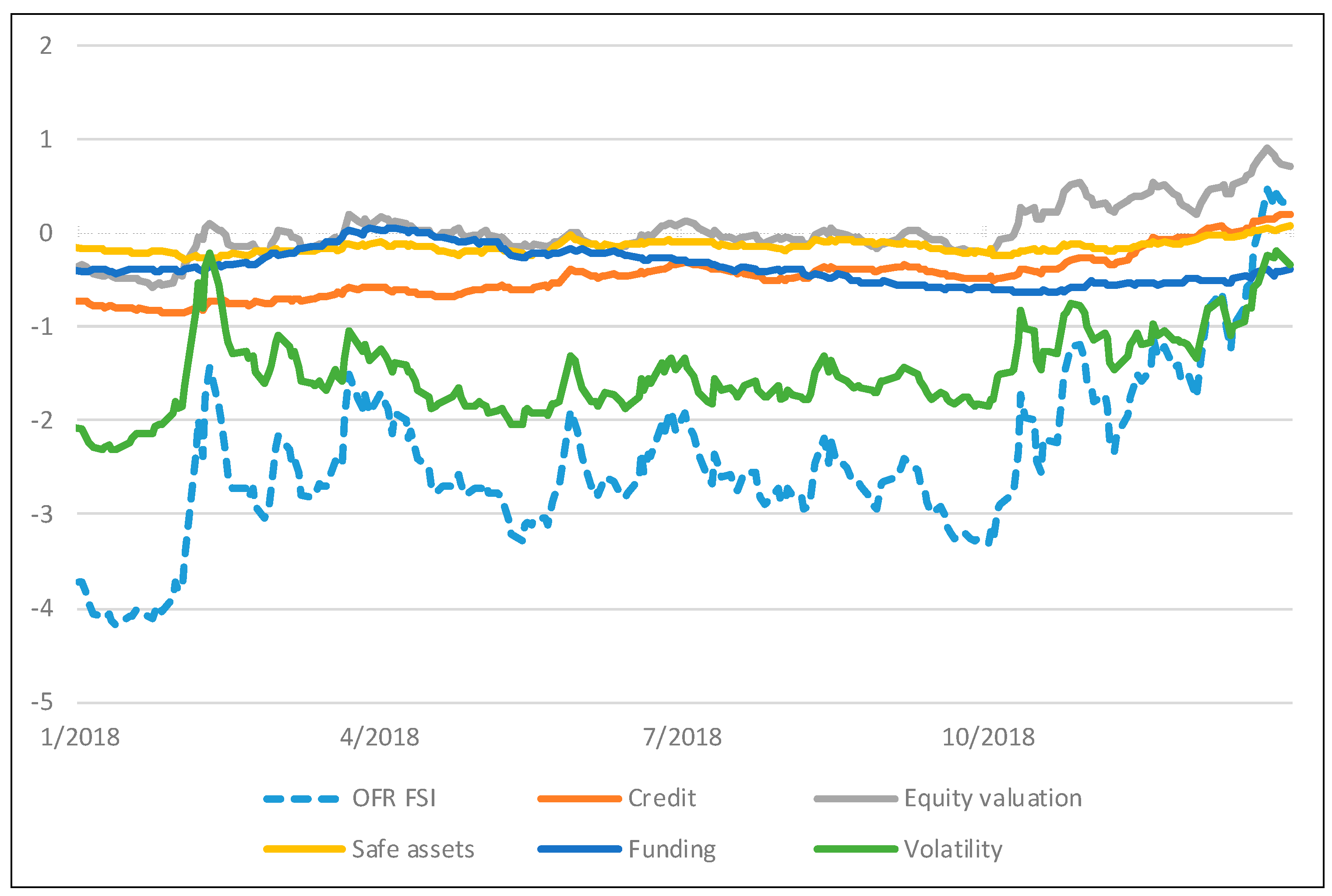
The OFR FSI shows stress at the beginning of 2018 at its lowest level since the global financial crisis of 2007–2009. Aside from an event in February during which volatility temporarily spiked, stress levels were essentially flat for the first three quarters of 2018 at levels that were well below average. As Figure 5 shows, the low stress was driven mostly by low volatility across global equity, fixed income, currency and commodity markets. Stress contributions from most other categories of the index were also negative. Low stress levels do not necessarily imply low levels of risk. During low stress periods, stress can build up endogenously as the environment may incentivize investors to take on more leverage and reach for yield.6 Thus, while the OFR FSI suggests that stress levels were low, this does not mean that risk or systemic risk was low. For information about the potential vulnerabilities in the financial system during 2018, we refer the reader to the OFR’s Financial System Vulnerabilities Monitor.
Financial stress increased dramatically in the fourth quarter of 2018, ending the year at its highest level in more than two years. The increase was most pronounced in the volatility, equity valuation, and credit subcategories of the index. The safe assets category also increased modestly, while the stress contribution from the funding subcategory remained relatively constant at below average levels. These changes reflect the changing risk sentiment in financial markets seen during the quarter. After a rough October and a tepid November, U.S. equities dropped almost 10 percent in December amid much higher market volatility. Credit spreads also widened during the quarter.
5. Stress Identification and the Relationship of Stress to Economic Activity
Previous sections described how the OFR FSI measures systemic financial stress. In this section we aim to empirically test this. This task is challenging because financial stress is a latent indicator in the economy. Following Carlson et al. (2012), we develop a proxy for global financial stress events using dates of significant government intervention. We show that higher values of the OFR FSI are associated with an increased likelihood of a financial stress event, evidence that the index measures financial stress. Next, we examine the relationship between financial stress and real economic activity. We find that higher values of the OFR FSI help predict decreased real economic activity, but not vice-versa. The analysis suggests that the OFR FSI performs well in identifying stress episodes, and that financial stress can have real economic effects.
5.1. Stress Identification Using the OFR FSI
The OFR FSI is designed to be a coincident indicator of stress in the global financial system. A natural question is how well it fulfills its intended purpose. As financial stress is unobserved and subject to interpretation, one challenge in evaluating whether the OFR FSI identifies financial stress periods is the lack of a natural or obvious benchmark for comparison. Some researchers have identified financial stress periods based on opinion (Nelson and Perli 2007; Illing and Liu 2006) while others have identified systemic events as states of abnormal equity returns (Dattels et al. 2010; Arsov et al. 2013). We adapt the approach in Carlson et al. (2012) that identifies U.S. financial stress as periods of “interventions by policymakers that occurred out of concern that troubles at a U.S. financial institution or the impairment in functioning of a U.S. financial market might present systemic risks to financial stability and have negative consequence for economic activity.” This approach identifies periods in which institutions or markets as a whole pose enough risk to the stability of the financial system that policymakers are persuaded to intervene. Carlson and coauthors select dates when the Federal Reserve, the Federal Deposit Insurance Corporation, or the Treasury Department interceded directly with an institution or market. The types of interventions are broad and include all actions taken by policymakers to protect market functioning.
In addition to the U.S.-centric intervention dates identified by Carlson et al. (2012), we add an international aspect to assess the global scope intended for the OFR FSI. Specifically, we identify dates in the eurozone starting in 2010 when the European Central Bank, International Monetary Fund, or a eurozone sovereign intervened or implemented policy due to concerns about potential risks to financial stability and spillover effects. Using a Euro crisis timeline compiled by a European think tank (Bruegel 2017), we compile dates since 2010 of intervention in European fiscal matters and financial markets and update the list through August 2017. A complete list of the government intervention dates is in Appendix B.
To test how well the OFR FSI identifies financial stress episodes, we run a logistic regression to assess the performance of the index in stress episodes defined by the intervention dates. The independent variable in the regression is the OFR FSI. The dependent variable, StressEvent, is a binary indicator with a daily frequency that is set at one in the four weeks before and after an intervention takes place, and otherwise set at zero. As in Carlson et al. (2012), we consider stress episodes to extend from four weeks before an intervention date to four weeks after. This captures stress leading up to the intervention, and market reaction and policy implementation following the intervention. The qualitative results of the logistic regression are not sensitive to the choice of window.
Descriptive statistics for the OFR FSI and the StressEvent are in Table 3. Both series are at a daily frequency from the inception of the OFR FSI on 3 January 2000 to 31 August 2017. During this period, the OFR FSI has, on average, been positive, with a mean of 0.76. Approximately one quarter of the daily observations of StressEvent are equal to one, indicating that the system has been experiencing financial stress for approximately one quarter of the sample period.
The logistic regression results are in Table 4. Standard errors for the estimated coefficients were computed using the moving block bootstrap method. We see from the table that the coefficient on the OFR FSI is positive and statistically significant, with a p-value well below 0.0001. The area under the curve of the receiver operator characteristic is 0.76. The results suggest that higher levels of the OFR FSI are associated with being in periods of financial stress. In addition, the odds ratio of 1.31 suggests that the financial system is 1.31 times as likely to be in a stress episode for every one unit increase in the OFR FSI. Finally, the McFadden’s pseudo R-squared value of 0.19 suggests that a moderate amount of the variation in StressEvent is explained by the OFR FSI.7 The analysis confirms the usefulness of the OFR FSI as a coincident indicator of systemic financial stress.
5.2. The Relationship of Financial Stress to Real Economic Activity
We have argued that the OFR FSI measures financial stress, a latent indicator in the economy, and have provided statistical evidence that supports this. One of the motivations in measuring financial stress is that it can have adverse real economic effects. This can occur in several ways. In times of increased uncertainty, firms and households may delay or reduce hiring, investment, and spending. Investors may sell riskier investments and buy safer ones, contributing to market illiquidity and increased asymmetric information. All these actions can result in increased borrowing costs and tightened credit standards, leading to a reduction in spending and economic activity (Hakkio and Keeton 2009).
Financial stress, as measured by other FSIs, can forecast declines in economic activity (see, among others, Kliesen et al. 2012, and Apostolakis and Papadopoulos 2019). Having shown that the OFR FSI is fit for its intended purpose of measuring financial stress, we can empirically test whether increases in financial stress, as measured by the OFR FSI, lead to decreases in economic activity. As in Hakkio and Keeton (2009), we use the Chicago Fed National Activity Index (CFNAI) (Chicago Fed National Activity Index 2016) as a proxy for overall economic activity. The monthly CFNAI is computed as a weighted average of 85 indicators of U.S. national economic activity drawn from four categories: production and income; employment, unemployment, and hours worked; consumption and housing; and sales, orders, and inventories. The CFNAI tracks periods of economic expansion and contraction, and periods of changing inflationary pressure.
Descriptive statistics of the OFR FSI and the CFNAI are in Table 5. To accommodate the monthly frequency of the CFNAI, the OFR FSI is downsampled to a monthly index using the last observation each month. There are 211 monthly observations between January 2000 and July 2017, inclusive. The OFR FSI had an average monthly value of 0.78, which is consistent with an average negative value for the CFNAI of −0.29. The OFR FSI has a substantially larger range than the CFNAI and there is a high negative correlation of −0.74 between the two indexes, as expected.
We use Granger non-causality analysis to test whether higher values of financial stress help predict decreases in economic activity. This technique involves setting up a regression model where each indicator is regressed on the past values of the other indicator. After properly specifying such a model to account for potential non-stationarity (Toda and Yamamoto 1995), the coefficients on the past values of the independent variable that are statistically significantly different from zero suggest that past values of that variable are helpful for predicting current values of the dependent variable.
The results from our analysis are in Table 6. The top panel reports the results of testing to see whether past values of the OFR FSI help to predict the CFNAI. The null hypothesis of the F-test that lagged values of the OFR FSI are not different from zero is soundly rejected with a p-value less than 0.0001. The coefficient estimates on the lagged values of the OFR FSI are negative. This suggests that decreases in the OFR FSI help to predict increases in the CFNAI. The bottom panel of Table 6 reports the results of whether past values the CFNAI help to predict the OFR FSI. In this case, the null hypothesis that the CFNAI does not Granger cause the OFR FSI cannot be rejected at the 5 percent level. This suggests that past values of the CFNAI do not help to predict the OFR FSI. Overall, the results show that increases in the OFR FSI help predict decreases in the CFNAI (and not vice versa), suggesting that the OFR FSI is useful for predicting reductions in overall economic activity.
6. Conclusions
The 2007–2009 global financial crisis showed how severe financial stress events can have devastating real economic consequences. Accordingly, measuring financial stress is of first-order importance to regulators and market participants alike. This paper introduces a new financial stress index, the OFR FSI. The OFR FSI is a daily, market-based snapshot of stress in global financial markets. It distills information from multiple stress categories and regions, offering insight into the drivers of stress. It helps the OFR monitor, compare, and understand financial stress events. The index offers improvements on other FSIs, including its decomposition into stress categories and a dynamic construction that allows for changes in variable composition and cross-asset relationships. Empirical results suggest that the OFR FSI successfully identifies financial stress events and helps predict changes in overall economic activity.
The OFR FSI is an entry point for financial market monitoring, not a sufficient statistic for understanding financial markets or financial stress events. It is a coincident indicator of stress in the financial system, not necessarily a leading indicator or predictor of financial stress events. In these respects, its limitations are analogous to those of body temperature, which provides the physician a summary statistic for a patient’s current condition that is correlated with sickness or other maladies but must be considered in tandem with other data to make the correct diagnosis. Similarly, the OFR FSI is considered alongside the OFR’s Financial System Vulnerabilities Monitor, and other data sources and factors to produce the OFR’s financial stability assessments.
Future research on the OFR FSI mainly concerns the set of its constituent indicators, which is not necessarily fixed. Indeed, the OFR FSI’s methodology allows the component list of indicators to change over time as the financial system evolves. For example, the removal of LIBOR as a meaningful reference rate over the next few years may necessitate the replacement of the LIBOR-based indicators currently in the index with other indicators that better reflect funding stress.
Funding
This research received no external funding.
Acknowledgments
An earlier version of the index was developed in collaboration with Thomas Piontek and William Shi. I thank Rebecca McCaughrin, Adam Minson, Kevin Sheppard, seminar participants at the Office of Financial Research, and the Office of Financial Research’s Financial Research Advisory Committee members for helpful comments and suggestions. I also thank Jonathan Glicoes for helpful research assistance.
Conflicts of Interest
The author declares no conflict of interest.
Appendix A

Table A1.
Variables in the OFR FSI.
| Category | Indicator | Region(s) | Source | First Date in FSI | Note | Exp. Sign |
|---|---|---|---|---|---|---|
| Credit | BaML US Corporate Master (IG) (OAS) | US | Haver | 1 January 2000 | L | Pos. |
| BaML US High Yield Corporate Master (HY) (OAS) | US | Haver | 1 January 2000 | L | Pos. | |
| BaML Euro Area Corp Bond Index (OAS) | AE | Haver | 1 January 2000 | L | Pos. | |
| BaML Euro Area High Yield Bond Index (OAS) | AE | Haver | 1 January 2000 | L | Pos. | |
| BaML Japan Corporate (OAS) | AE | Haver | 1 January 2000 | L | Pos. | |
| JPMorgan CEMBI Strip Spread | EM | Bloomberg | 1 January 2004 | L | Pos. | |
| JPMorgan EMBI Global Strip Spread | EM | Bloomberg | 1 April 2003 | L | Pos. | |
| Equity Valuation | MSCI Emerging Markets Index (P/B Ratio) | EM | Bloomberg | 1 January 2000 | LRMA | Neg. |
| MSCI Europe Index (P/B Ratio) | AE | Bloomberg | 1 February 2001 | LRMA | Neg. | |
| NIKKEI 225 Index (P/B Ratio) | AE | Bloomberg | 1 May 2002 | LRMA | Neg. | |
| S&P 500 Index (P/B Ratio) | US | Bloomberg | 1 January 2000 | LRMA | Neg. | |
| Funding | 2-Year EUR/USD Cross-Currency Swap Spread | US, AE | Bloomberg | 1 February 2001 | L | N/A |
| 2-Year US Swap Spread | US | Bloomberg | 1 January 2000 | L | N/A | |
| 2-Year USD/JPY Cross-Currency Swap Spread | US, AE | Bloomberg | 1 January 2000 | L | N/A | |
| 3-Month EURIBOR—EONIA | AE | Bloomberg, Haver | 1 March 2002 | L | Pos. | |
| 3-Month Japanese LIBOR—OIS | AE | Bloomberg | 1 April 2004 | L | Pos. | |
| 3-Month LIBOR—OIS | US | Bloomberg | 1 January 2004 | L | Pos. | |
| 3-Month TED Spread | US | Bloomberg | 1 January 2000 | L | Pos. | |
| Safe Assets | 10-Year US Treasury Note (yield) | US | Haver | 1 January 2000 | DMA | Neg. |
| 10-Year German Bond (yield) | AE | Bloomberg | 1 January 2000 | DMA | Neg. | |
| Gold/USD Real Spot Exchange Rate | US, AE, EM | Haver | 1 January 2000 | LRMA | Pos. | |
| Japanese Yen/USD Spot Exchange Rate | AE | Haver | 1 January 2000 | LRMA | N/A | |
| Swiss Franc/USD Spot Exchange Rate | AE | Haver | 1 January 2000 | LRMA | N/A | |
| US Dollar Index (DXY) | US | Bloomberg | 1 January 2000 | LRMA | N/A | |
| Volatility | CBOE S&P 500 Volatility Index (VIX) | US | Haver | 1 January 2000 | L | Pos. |
| Dow Jones EURO STOXX 50 Volatility Index (V2X) | AE | Bloomberg | 1 March 2002 | L | Pos. | |
| ICE Brent Crude Oil Futures (22-day realized vol.) | US, AE, EM | Bloomberg | 1 January 2000 | L | Pos. | |
| Implied Volatility on 6-Month EUR/USD Options | US, AE | Bloomberg | 1 February 2001 | L | Pos. | |
| Implied Volatility on 6-Month USD/JPY Options | US, AE | Bloomberg | 1 January 2000 | L | Pos. | |
| JPMorgan Emerging Market Volatility Index | AE | Bloomberg | 1 April 2003 | L | Pos. | |
| Merrill Lynch Euro Swaptions Volatility Estimate | AE | Bloomberg | 1 January 2000 | L | Pos. | |
| Merrill Lynch US Swaptions Volatility Estimate | US | Bloomberg | 1 January 2000 | L | Pos. | |
| NIKKEI Volatility Index | AE | Bloomberg | 1 February 2003 | L | Pos. | |
| Key | ||||||
| AE = Advanced economies ex-U.S., e.g., eurozone and Japan | HY = High yield | |||||
| BaML = Bank of America Merrill Lynch | IG = Investment grade | |||||
| CBOE = Chicago Board Options Exchange | JPY = Japanese yen | |||||
| CEMBI = Corporate Emerging Markets Bond Index | LIBOR = London Interbank Offered Rate | |||||
| EM = Emerging markets | MSCI = Morgan Stanley Capital International | |||||
| EMBI = Emerging Market Bond Index | OAS = Option-adjusted spread | |||||
| EONIA = Euro OverNight Index Average | OIS = Overnight indexed swap | |||||
| EUR = Euro | P/B Ratio = Price-to-book ratio (value-weighted) | |||||
| EURIBOR = Euro InterBank Offered Rate | USD = U.S. dollar | |||||
L = level; DMA = difference of the indicator and its 250-trading day moving average; LRMA = logarithm of the ratio of the indicator to its 250-trading day moving average; All variables are at a daily frequency, using values at market close.
Appendix B
Table A2.
Dates of Signficant Government Intervention in Financial Markets.
| Date | Intervention |
|---|---|
| 23 September 1998 | Federal Reserve coordinates purchase of LTCM by consortium of 12 firms |
| 11 September 2001 | Federal Reserve responds to liquidity shortages caused by the physical limitations of 9/11 |
| 10 August 2007 | Federal Reserve adds $38 billion in reserves and issues a statement reaffirming its commitment to provide liquidity |
| 17 August 2007 | Federal Reserve reduces primary credit spread by 50 basis points and allows 30-day term financing |
| 21 August 2007 | Federal Reserve reduced minimum fee rate for SOMA securities lending |
| 26 November 2007 | Federal Reserve eases terms on SOMA lending |
| 12 December 2007 | Federal Reserve announced creation of the TAF |
| 7 March 2008 | Federal Reserve announces it is expanding the size of the next two TAF auctions |
| 11 March 2008 | Federal Reserve announces the creation of the TSLF |
| 14 March 2008 | Federal Reserve lends to Bear Stearns |
| 16 March 2008 | Federal Reserve facilitates purchase of Bear Stearns by JPMC and creates PDCF |
| 2 May 2008 | Federal Reserve increases the size of TAF auctions |
| 13 July 2008 | Federal Reserve authorizes the Federal Reserve Bank of New York to lend to Fannie and Freddie should lending prove necessary |
| 30 July 2008 | Federal Reserve extends term lending on TAF to 84 days |
| 7 September 2008 | Treasury places Fannie and Freddie into conservatorship and provides liquidity backstops for GSEs |
| 15 September 2008 | Federal Reserve expands PDCF eligible assets and conducts two open market operations |
| 16 September 2008 | Federal Reserve extends line of credit to AIG |
| 19 September 2008 | Federal Reserve announces AMLF and Treasury guarantees MMMFs |
| 28 September 2008 | FDIC announces assistance for Wachovia merger and Federal Reserve increase size of TAF |
| 6 October 2008 | Federal Reserve further expands size of TAF |
| 7 October 2008 | Federal Reserve announces creation of the CPFF |
| 8 October 2008 | Federal Reserve decreases fees on SOMA lending |
| 14 October 2008 | Treasury announces $250 billion for preferred stock purchases and FDIC announces TLGP |
| 21 October 2008 | Federal Reserve announces the creation of the MMIFF |
| 23 November 2008 | Federal Reserve, Treasury, and FDIC agree to provide Citigroup a package of guarantees, liquidity access, and capital |
| 25 November 2008 | Federal Reserve announces the TALF |
| 30 December 2008 | Treasury announces the purchase of preferred stock in GMAC |
| 7 January 2009 | Federal Reserve expands set of institutions eligible to borrow under the MMIFF |
| 16 January 2009 | Treasury, FDIC, and Federal Reserve provide Bank of America with rescue package |
| 30 January 2009 | Federal Reserve liberalizes rules related to AMLF |
| 25 February 2009 | Federal Reserve, OCC, FDIC, and OTS announce details of the Capital Assistance Program |
| 23 March 2009 | Treasury announces the details of the public-partnership investment plan |
| 1 May 2009 | Federal Reserve announces the inclusion of the CMBS in the TALF |
| 7 May 2009 | Bank stress test results and capital-raising requirements for SCAP firms officially announced |
| 19 May 2009 | Federal Reserve further expands collateral eligible under the TALF |
| 2 May 2010 | Euro area member states and the IMF announce a three-year program for Greece, totaling €110 billion |
| 9 May 2010 | Euro area leaders announce that all the institutions of the euro area, including the ECB, commit to an overhaul of the European macroeconomic surveillance framework. Finance ministers announce the creation of the European Financial Stability Facility |
| 11 May 2010 | Federal Reserve agrees with foreign central banks to reestablish temporary dollar swap facilities |
| 29 October 2010 | European leaders reach an agreement on the need to set up a permanent crisis mechanism to safeguard the financial stability of the euro area as a whole (the European Stability Mechanism or ESM) |
| 28 November 2010 | European leaders and the IMF agree to grant an €85 billion assistance package to Ireland |
| 11 March 2011 | Euro area leaders agree to make the EFSF’s €440 billion lending capacity fully effective, and to allow the EFSF and ESM to intervene in the primary markets for sovereign debt, as an exception and only in the context of a financial assistance program |
| 17 May 2011 | Having received a request from Portugal, the European Council agrees to a financial assistance package totaling €78 billion over three years |
| 21 July 2011 | Euro area Heads of State or Government and EU institutions decide on a new package of measures to end the crisis and prevent contagion, including: a new program for Greece, and an agreement hat includes measures to enhance the flexibility of stabilization tolls by allowing the EFSF/ESM to act on the basis of a precautionary program, to intervene in secondary markets, and to finance the recapitalization of financial institutions through loans to governments, including non-program countries |
| 4 August 2011 | The ECB reactivates secondary market purchases and starts purchasing Italian and Spanish bonds in an attempt to ease market tensions |
| 6 September 2011 | The Swiss Central Bank announces its decision to cap the Swiss franc’s euro exchange rate, in an attempt to halt its appreciation |
| 27 October 2011 | European leaders agree on another comprehensive package of additional measures, focused on Greece and European firewalls. Leaders also agree to “optimize” the resources of the EFSF by introducing two leverage options, allowing the EFSF’s firepower to be multiplied |
| 30 November 2011 | The ECB, the Fed, the Bank of Japan, the Bank of England, and the Swiss National Bank announce agreement to enhance their ability to provide liquidity. The agreement involves the extension of these arrangements to February 2013 and the possibility for each of the central banks to provide liquidity support in any of their currencies |
| 8 December 2011 | The ECB announces a package of measures to support the banking system, including the long-term refinancing operations |
| 21 February 2012 | European leaders agree on the terms for a second rescue program for Greece, with a marginally higher contribution from the private sector |
| 12 March 2012 | The Spanish government adopts a new comprehensive package of measures to strengthen the banking sector |
| 9 June 2012 | Spain becomes the first country to request financial assistance to recapitalize its banking sector, within the framework of a €100 billion program focused on the banking sector only |
| 25 June 2012 | Cyprus formally requests financial assistance form the EU and IMF |
| 30 April 2014 | the IMF approves a loan of $17.01 billion to Ukraine under a two-year Stand-by Arrangement in order to support Ukraine’s economic reform program |
| 15 January 2015 | The Swiss Central Bank abandons its currency cap against the euro as expectations for an ECB quantitative easing program put pressure on the Swiss franc |
| 11 March 2015 | The IMF approves a new loan of $17.5 billion to Ukraine to stabilize the economy and financial sector, bringing the total bailout package to $40 billion over four years |
| 14 August 2015 | Eurozone finance ministers agree to a third Greek bailout package worth €86 billion in exchange for tax hikes and spending cuts |
| 4 August 2016 | Bank of England launches four stimulating measures in response to Brexit |
Sources: Carlson et al. (2012), Bruegel, OFR analysis.
References
- Acharya, Viral V., Lasse H. Pedersen, Thomas Philippon, and Matthew Richardson. 2017. Measuring Systemic Risk. Review of Financial Studies 30: 2–47. [Google Scholar] [CrossRef]
- Adam, Tomáš, Soňa Benecká, and Jakub Matějů. 2018. Financial stress and its non-linear impact on CEE exchange rates. Journal of Financial Stability 36: 346–60. [Google Scholar] [CrossRef]
- Adrian, Tobias, and Markus K. Brunnermeier. 2016. CoVaR. American Economic Review 106: 1705–41. [Google Scholar] [CrossRef]
- Apostolakis, George, and Athanasios P. Papadopoulos. 2019. Financial Stability, Monetary Stability and Growth: A PVAR Analysis. Open Economies Review 30: 157–78. [Google Scholar] [CrossRef]
- ARRC. 2017. The ARRC Selects a Broad Repo Rate as its Preferred Alternative Reference Rate. ARRC: Alternative Reference Rates Committee. Press Release. June 22. Available online: https://www.newyorkfed.org/arrc/announcements.html (accessed on 23 October 2017).
- Arsov, Ivailo, Elie Canetti, Laura E. Kodres, and Srobona Mitra. 2013. Near-Coincident Indicators of Systemic Stress. IMF Working Paper No. 13/115, International Monetary Fund, Washington, DC, USA. May 17. [Google Scholar]
- Bai, Jushan, and Serena Ng. 2008. Large Dimensional Factor Analysis. Foundations and Trends in Econometrics 3: 89–163. [Google Scholar] [CrossRef] [Green Version]
- Bisias, Dimitrios, Mark Flood, Andrew W. Lo, and Stavros Valavanis. 2012. A Survey of Systemic Risk Analytics. OFR Working Paper No. 12-01, Office of Financial Research, Washington, DC, USA. January 5. [Google Scholar]
- Brave, Scott A., and R. Butters. 2011. Monitoring Financial Stability: A Financial Conditions Approach. Economic Perspectives 35: 22–43. [Google Scholar]
- Bruegel. 2017. Euro Crisis Timeline. Available online: http://www.bruegel.org (accessed on 23 October 2017).
- Cardarelli, Roberto, Selim Elekdag, and Subir Lall. 2011. Financial Stress and Economic Contractions. Journal of Financial Stability 7: 78–97. [Google Scholar] [CrossRef]
- Carlson, Mark, Kurt Lewis, and William Nelson. 2012. Using Policy Intervention to Identify Financial Stress. Finance and Economics Discussion Series Working Paper 2012-02, Federal Reserve Board, Washington, DC, USA. January 10. [Google Scholar]
- Chicago Fed National Activity Index. 2016. Online Content, December 22. Available online: https://www.chicagofed.org/publications/cfnai/index (accessed on 23 October 2017).
- Dattels, Peter, Rebecca McCaughrin, Ken Miyajima, and Jaume Puig. 2010. Can You Map Global Financial Stability? IMF Working Paper No. 2010/145, International Monetary Fund, Washington, DC, USA. June. [Google Scholar]
- Duprey, Thibaut, and Benjamin Klaus. 2017. How to predict financial stress? An assessment of Markov switching models. ECB Working Paper Series No. 2057, European Central Bank, Frankfurt, Germany. May. [Google Scholar]
- Duprey, Thibaut, Benjamin Klaus, and Tuomas Peltonen. 2017. Dating systemic financial stress episodes in EU countries. Journal of Financial Stability 32: 30–56. [Google Scholar] [CrossRef]
- Grimaldi, Marianna B. 2010. Detecting and Interpreting Financial Stress in the Euro Area. ECB Working Paper Series No. 1214, European Central Bank, Frankfurt, Germany. June. [Google Scholar]
- Grimaldi, Marianna B. 2011. Up for Count? Central Bank Words and Financial Stress. Sveriges Riksbank Working Paper Series No. 252, Sveriges Riksbank, Stockholm, Sweden. April. [Google Scholar]
- Hakkio, Craig S., and William R. Keeton. 2009. Financial stress: What is it, how can it be measured, and why does it matter? Economic Review 94: 5–52. [Google Scholar]
- Hatzius, Jan, Peter Hooper, Frederic S. Mishkin, Kermit L. Schoenholtz, and Mark W. Watson. 2010. Financial Conditions Indexes: A Fresh Look after the Financial Crisis. NBER Working Paper 16150, National Bureau of Economic Research, Cambridge, MA, USA. July. [Google Scholar]
- Hollo, Daniel, Manfred Kremer, and Marco Lo Duca. 2012. CISS—A Composite Indicator of Systemic Stress in the Financial System. ECB Working Paper Series No. 1426, European Central Bank, Frankfurt, Germany. March. [Google Scholar]
- Huang, Xin, Hao Zhou, and Haibin Zhu. 2012. Assessing the systemic risk of a heterogeneous portfolio of banks during the recent financial crisis. Journal of Financial Stability 8: 193–205. [Google Scholar] [CrossRef]
- Illing, Mark, and Ying Liu. 2006. Measuring Financial Stress in a Developed Country: An Application to Canada. Journal of Financial Stability 2: 243–65. [Google Scholar] [CrossRef]
- Kliesen, Kevin L., and Douglas C. Smith. 2010. Measuring Financial Market Stress. Federal Reserve Bank of St. Louis National Economic Trends, January 15. [Google Scholar]
- Kliesen, Kevin L., Michael T. Owyang, and E. Katarina Vermann. 2012. Disentangling Diverse Measures: A Survey of Financial Stress Indexes. Federal Reserve Bank of St. Louis Review 94: 369–97. [Google Scholar] [CrossRef]
- Lo Duca, Marco, and Tuomas A. Peltonen. 2011. Macro-Financial Vulnerabilities and Future Financial Stress: Assessing Systemic Risks and Predicting Systemic Events. ECB Working Paper Series No. 1311, European Central Bank, Frankfurt, Germany. March. [Google Scholar]
- Louzis, Dimitrios P., and Angelos T. Vouldis. 2013. A Financial Systemic Stress Index for Greece. ECB Working Paper No 1563, European Central Bank, Frankfurt, Germany. July. [Google Scholar]
- McFadden, Daniel. 1977. Quantitative Methods for Analyzing Travel Behaviour of Individuals: Some Recent Developments. Cowles Foundation Discussion Paper No. 474. New Haven: Cowles Foundation for Research in Economics at Yale University, November 22. [Google Scholar]
- Nelson, William R., and Roberto Perli. 2007. Selected Indicators of Financial Stability. Risk Management and Systemic Risk 4: 343–72. [Google Scholar]
- OFR Financial Markets Monitor. 2017. The Volatility Paradox: Tranquil Markets May Harbor Hidden Risks. Second Quarter 2017. August 17. Available online: https://www.financialresearch.gov/financial-markets-monitor/2017/08/17/the-volatility-paradox/ (accessed on 23 October 2017).
- Rosenberg, Michael. 2009. Financial Conditions Watch: Global Financial Market Trends and Policy. Bloomberg LLP, September 11. [Google Scholar]
- Sandahl, Johannes F., Mia Holmfeldt, Anders Rydén, and Maria Strömqvist. 2011. An Index of Financial Stress for Sweden. Sveriges Riksbank Economic Review 2: 49–67. [Google Scholar]
- Stock, James H., and Mark Watson. 2002. Macroeconomic Forecasting Using Diffusion Indexes. Journal of Business & Economic Statistics 20: 147–62. [Google Scholar]
- Stock, James H., and Mark Watson. 2006. Forecasting with Many Predictors. In Handbook of Economic Forecasting. Edited by Graham Elliot, Clive Granger and Allan Timmermann. Amsterdam: Elsevier, chp. 6. pp. 515–54. [Google Scholar]
- Stock, James H., and Mark Watson. 2010. Dynamic Factor Models. In Oxford Handbook of Economic Forecasting. Edited by Michael Clements and David Hendry. Oxford: Oxford University Press. [Google Scholar]
- Toda, Hiro Y., and Taku Yamamoto. 1995. Statistical inference in vector autoregressions with possibly integrated processes. Journal of Econometrics 66: 225–50. [Google Scholar] [CrossRef]
- Vasicek, Borek, Diana Zigraiova, Marco Hoeberichts, Robert Vermeulen, Katerina Smidkova, and Jakob de Haan. 2017. Leading indicators of financial stress: New evidence. Journal of Financial Stability 28: 240–57. [Google Scholar] [CrossRef]
| 1 | The OFR Financial Stress Index (OFR FSI) is published after every U.S. trading day by the Office of Financial Research. It is available online at https://www.financialresearch.gov/financial-stress-index/. |
| 2 | |
| 3 | This proceeds as follows: initialize the algorithm with a loading vector and compute an initial factor . Subsequent iterates are computed using and . We proceed for 200 iterations. We then repeat the analysis 15 times, initializing the vector in different ways, including taking the first principal component of the largest subset of balanced panel data, taking the first principal component using a pseudo-correlation matrix constructed by the pairwise correlations using each pair’s overlapping sample, and sampling from a random normal vector. We then select the iteration with the smallest sum of squared errors. |
| 4 | Descriptions of the indicator categories are in Table 1. Additional information about the indicators in the index, including definitions of the abbreviations used in Table 2, is available in Appendix A. |
| 5 | The 10-year Treasury note yield is transformed to be relative to its 250-trading day moving average. See Appendix A. |
| 6 | See for example, (OFR Financial Markets Monitor 2017) “The Volatility Paradox: Tranquil Markets May Harbor Hidden Risks.” |
| 7 | McFadden’s pseudo R-squared is equal to one minus the ratio of the log-likelihood of the model containing the OFR FSI to that of the model with just a constant. Higher values are thus associated with more variation in StressEvent being explained by the OFR FSI. McFadden (1977) suggests that values above 0.2 indicate “excellent” model fit. |
Figure 1.
The OFR FSI between January 2000 and December 2018.

Figure 2.
Decomposition of the OFR FSI during the 2007–2009 Global Financial Crisis.

Figure 3.
Decomposition of the OFR FSI during European Sovereign Debt Crisis.

Figure 4.
Decomposition of the OFR FSI during European Sovereign Debt Crisis, By Region.

Figure 5.
Decomposition of the OFR FSI in 2018.

Table 1.
OFR FSI indicator category definitions.
| Category | Definition |
|---|---|
| Credit | Contains measures of credit spreads, which represent the difference in borrowing costs for firms of different creditworthiness. In times of stress, credit spreads may widen when default risk increases or credit market functioning is disrupted. Wider spreads may indicate that investors are less willing to hold debt, increasing costs for borrowers to get funding. |
| Equity valuation | Contains stock valuations from several stock market indexes, which reflect investor confidence and risk appetite. In times of stress, stock values may fall if investors become less willing to hold risky assets. |
| Funding | Contains measures related to how easily financial institutions can fund their activities. In times of stress, funding markets can freeze if participants perceive greater counterparty credit risk or liquidity risk. |
| Safe assets | Contains valuation measures of assets that are considered stores of value or have stable and predictable cash flows. In times of stress, higher valuations of safe assets may indicate that investors are migrating from risky or illiquid assets into safer holdings. |
| Volatility | Contains measures of implied and realized volatility from equity, credit, currency, and commodity markets. In times of stress, rising uncertainty about asset values or investor behavior can lead to higher volatility. |
Table 2.
Decomposition of the OFR FSI on 31 December 2018.
| Indicator Category | Indicator | Coef. | Data | Wgt. | Data * | Contr. | Subtotal |
|---|---|---|---|---|---|---|---|
| Credit | BaML US Corporate Master (IG) (OAS) | 0.241 | 0.016 | 0.241 | 0.016 | 0.004 | |
| BaML US High Yield Corporate Master (HY) (OAS) | 0.244 | −0.114 | 0.244 | −0.114 | −0.028 | ||
| BaML Euro Area Corp Bond Index (OAS) | 0.160 | 0.761 | 0.160 | 0.761 | 0.122 | ||
| BaML Euro Area High Yield Bond Index (OAS) | 0.230 | −0.346 | 0.230 | −0.346 | −0.080 | ||
| BaML Japan Corporate (OAS) | 0.174 | 0.697 | 0.174 | 0.697 | 0.122 | ||
| JPMorgan CEMBI Strip Spread | 0.209 | 0.248 | 0.209 | 0.248 | 0.052 | ||
| JPMorgan EMBI Global Strip Spread | 0.131 | 0.100 | 0.131 | 0.100 | 0.013 | 0.205 | |
| Equity Valuation | MSCI Emerging Markets Index (P/B Ratio) | −0.141 | −0.618 | 0.141 | 0.618 | 0.087 | |
| MSCI Europe Index (P/B Ratio) | −0.190 | −0.855 | 0.190 | 0.855 | 0.162 | ||
| NIKKEI 225 Index (P/B Ratio) | −0.172 | −1.102 | 0.172 | 1.102 | 0.190 | ||
| S&P 500 Index (P/B Ratio) | −0.197 | −1.365 | 0.197 | 1.365 | 0.269 | 0.708 | |
| Funding | 2-Year EUR/USD Cross-Currency Swap Spread | −0.095 | 0.244 | 0.095 | −0.244 | −0.023 | |
| 2-Year US Swap Spread | 0.174 | −0.960 | 0.174 | −0.960 | −0.167 | ||
| 2-Year USD/JPY Cross-Currency Swap Spread | −0.012 | −0.484 | 0.012 | 0.484 | 0.006 | ||
| 3-Month EURIBOR—EONIA | 0.206 | −0.579 | 0.206 | −0.579 | −0.120 | ||
| 3-Month Japanese LIBOR—OIS | 0.187 | −0.941 | 0.187 | −0.941 | −0.176 | ||
| 3-Month LIBOR—OIS | 0.192 | 0.407 | 0.192 | 0.407 | 0.078 | ||
| 3-Month TED Spread | 0.173 | 0.036 | 0.173 | 0.036 | 0.006 | −0.395 | |
| Safe Assets | 10-Year US Treasury Note (yield) | −0.105 | −0.301 | 0.105 | 0.301 | 0.032 | |
| 10-Year German Bond (yield) | −0.095 | −0.190 | 0.095 | 0.190 | 0.018 | ||
| Gold/USD Real Spot Exchange Rate | 0.033 | −0.048 | 0.033 | −0.048 | −0.002 | ||
| Japanese Yen/USD Spot Exchange Rate | −0.109 | −0.023 | 0.109 | 0.023 | 0.002 | ||
| Swiss Franc/USD Spot Exchange Rate | −0.008 | 0.191 | 0.008 | −0.191 | −0.002 | ||
| US Dollar Index (DXY) | 0.050 | 0.547 | 0.050 | 0.547 | 0.027 | 0.076 | |
| Volatility | CBOE S&P 500 Volatility Index (VIX) | 0.254 | 0.790 | 0.254 | 0.790 | 0.201 | |
| Dow Jones EURO STOXX 50 Volatility Index (V2X) | 0.209 | −0.029 | 0.209 | −0.029 | −0.006 | ||
| ICE Brent Crude Oil Futures (22-day realized volatility) | 0.176 | 1.518 | 0.176 | 1.518 | 0.267 | ||
| Implied Volatility on 6-Month EUR/USD Options | 0.199 | −1.052 | 0.199 | −1.052 | −0.210 | ||
| Implied Volatility on 6-Month USD/JPY Options | 0.161 | −0.872 | 0.161 | −0.872 | −0.140 | ||
| JPMorgan Emerging Market Volatility Index | 0.216 | −0.169 | 0.216 | −0.169 | −0.037 | ||
| Merrill Lynch Euro Swaptions Volatility Estimate | 0.198 | −1.696 | 0.198 | −1.696 | −0.336 | ||
| Merrill Lynch US Swaptions Volatility Estimate | 0.185 | −0.922 | 0.185 | −0.922 | −0.170 | ||
| NIKKEI Volatility Index | 0.208 | 0.507 | 0.208 | 0.507 | 0.105 | −0.326 | |
| OFR FSI | 0.268 | ||||||
Note: “Coef.” provides the indicators’ weights in the loading vector of the dynamic factor model; “Data” provides the standardized values of the indicators on 31 December 2018; “Wgt.” is the absolute value of “Coef.”; “Data*” is the product of “Data” and the sign of “Coef.”; and “Contr.” Is the product of “Coef.” and “Data” or, equivalently, the product of “Wgt.” and “Data*.” Sources: Bloomberg Finance L.P., Haver Analytics, OFR analysis.
Table 3.
Descriptive statistics for the OFR FSI and StressEvent.
| Variable | Mean | Std | 25% | 50% | 75% |
|---|---|---|---|---|---|
| OFR FSI | 0.76 | 4.68 | −2.64 | −0.22 | 2.95 |
| Count = 0 | Count = 1 | ||||
| StressEvent | 3364 | 1081 |
Note: There are 4445 daily observations for each series from 3 January 2000 to 31 August 2017. Sources: Bloomberg Finance L.P., Bruegel, Carlson et al. (2012), Haver Analytics, OFR analysis.
Table 4.
Does the OFR FSI identify periods of financial stress?
| Dependent Variable: StressEvent | ||||
|---|---|---|---|---|
| Variable | Coef. | SE | t-stat | p-Value |
| Constant | −1.521 | 0.044 | −34.620 | <0.00001 |
| OFR FSI | 0.271 | 0.010 | 24.270 | <0.00001 |
| Odds ratio | 1.31 | |||
| McF-R2 | 0.19 | |||
| AUC | 0.76 | |||
Note: This table reports logistic regression results of StressEvent on the OFR FSI. McF-R2 refers to McFadden’s pseudo R-squared value and AUC refers to the area under the Receiver Operator Characteristic. Standard errors are calculated using the moving block bootstrap method. Sources: Bloomberg Finance L.P., Bruegel, Carlson et al. (2012), Haver Analytics, OFR analysis.
Table 5.
Descriptive statistics for the OFR FSI and Chicago Fed National Activity Index.
| Variable | Mean | Std | 25% | 50% | 75% |
| OFR FSI | 0.78 | 4.61 | −2.49 | −0.22 | 3.02 |
| CFNAI | −0.29 | 0.85 | −0.51 | −0.16 | 0.19 |
Note: The OFR FSI is downsampled to a monthly frequency using the last observation for a given month. There are 211 monthly observations. The correlation between the two series is −0.74. Sources: Bloomberg Finance L.P., Haver Analytics, OFR analysis.
Table 6.
Does financial stress help predict reductions in economic activity?
| Dependent Variable: CFNAI | |||
| Variable | Coef. | SE | t-stat |
| OFR FSI (t−1) | −0.036 | 0.023 | −1.521 |
| OFR FSI (t−2) | −0.071 | 0.035 | −2.043 |
| Does the OFR FSI help predict CFNAI? | |||
| Null hypothesis: OFR FSI does not Granger cause the CFNAI | |||
| F-stat | 13.30 | ||
| p-value | <0.0001 | ||
| Dependent Variable: OFR FSI | |||
| Variable | Coef. | SE | t-stat |
| CFNAI (t−1) | −0.392 | 0.212 | −1.849 |
| CFNAI (t−2) | 0.064 | 0.200 | 0.320 |
| Does the CFNAI help predict OFR FSI? | |||
| Null hypothesis: CFNAI does not Granger cause the OFR FSI | |||
| F-stat | 1.71 | ||
| p-value | 0.1835 | ||
Note: Table reports results from Granger non-causality testing performed using method of Toda and Yamamoto (1995). Lag length of 2 determined using the Bayesian Information Criterion. There are 211 monthly observations between January 2000 and July 2017. Sources: Bloomberg Finance L.P., Haver Analytics, OFR analysis.
© 2019 by the author. Licensee MDPI, Basel, Switzerland. This article is an open access article distributed under the terms and conditions of the Creative Commons Attribution (CC BY) license (http://creativecommons.org/licenses/by/4.0/).
Share and Cite
MDPI and ACS Style
Monin, P.J. The OFR Financial Stress Index. Risks 2019, 7, 25. https://doi.org/10.3390/risks7010025
AMA Style
Monin PJ. The OFR Financial Stress Index. Risks. 2019; 7(1):25. https://doi.org/10.3390/risks7010025
Chicago/Turabian StyleMonin, Phillip J. 2019. "The OFR Financial Stress Index" Risks 7, no. 1: 25. https://doi.org/10.3390/risks7010025
Note that from the first issue of 2016, this journal uses article numbers instead of page numbers. See further details here.