1. Introduction
Gartley (
1935) introduced the moving average (MA) trading rule to detect stochastic trends in the prices of risky assets. According to the rule, unnecessary price fluctuations are supposedly reduced when the rolling averages are calculated over the price history. If the rolling average is lower (higher) than the current closing price, the rule suggests that an uptrend (downtrend) prevails in risky asset prices.
Black (
1986) refined the idea of Gartley by assuming that all unnecessary price fluctuations that are independent of fundamental information concerning the risky assets were noise fluctuations (that is, opposite to those produced by fundamental information). This means that any price variation that has nothing to do with any new information regarding risky assets can simply be referred to as noise. This idea has become elementary in the behavioral finance literature that started from
Shiller (
1981), which asks why asset price fluctuations are more severe than expected fundamentals would count for.
Henriksson and Merton (
1981) stated that trading rules are usually used to determine when to buy or sell stocks, and calls this ‘market timing’. According to Merton, market timing by some technical trading rule is useless, and its performance should equal that of random market timing in efficient financial markets. Short selling costs or fund manager constraints make the market timing strategy usually turn into a simple rule, specifically when to buy risky assets, and when to sell them and switch to the risk-free asset.
The phenomenon is important because
Menkhoff (
2010) reports that 87% of fund managers use technical trading rules in their investment decisions, and tend to use the weekly horizon as the time frame. According to
Zhu and Zhou (
2009), the MA200 daily rule is the most popular trend chasing rule, in practice. This market timing rule means that the rolling window is 200 trading days, and every trading day is included in the calculations of the historical average.
Ilomäki et al. (
2018) used the Dow Jones Industrial Average (DJIA) stocks from the beginning of 1988 through to the end of 2017, and found that the lower was the frequency in the MA rule, the higher were average daily returns, even though average volatilities remained unchanged. The MA was calculated for the following frequencies: daily, weekly, monthly, every other month, every third month, every fourth month, and every fifth month, from the maximum 200 rolling window to the smallest. Monthly frequencies were produced, for example, with ten, nine, eight, seven, six, five, four, three, and two monthly observations. The largest rolling window (200 days) produced the best results, on average, with all frequencies including, for example, ten observations at the monthly frequency.
More importantly, the MA200 was found to produce a lower Sharpe ratio than the random market timing strategy, implying that the most popular MA rule among practitioners was useless for risk averse market timing. However, starting from the monthly frequency, that is, every 22nd trading day in the 200-day rolling window, the MA200 Sharpe ratio began to exceed that of the random timing strategy. Moreover, the Sharpe ratio continued to rise when the frequency was reduced. This suggests that the MA rules are more accurate in detecting long term stochastic trends.
The empirical results indicated an anomaly: lower frequency increases returns and Sharpe ratios with relatively unchanged volatility. The anomaly can be explained by the time varying risk premium of aggregate risk averse investors, or by investor affection for high volatility (see
Baker et al. 2011). The literature in financial economics discusses stock returns being predictable in the long run, as well as problems raised by the persistence of explanatory variable observations (mainly dividend yields and dividend-price ratios). Our procedure solves the problem by using only returns as observations.
In
Ilomäki et al. (
2018), the annualized average volatilities and average returns were calculated using annualized Sharpe ratios. This raises a question about conditional volatility that indicates time-varying risk. Among other issues, this paper tackles that question. In addition, what would happen to the performance if the rolling window size were expanded? What about long term stock return predictability? The null hypothesis is that the size of rolling windows or frequencies do not explain the performance of MA rules. The empirical results confirm previous empirical findings, namely that reduction of the frequency of the rolling windows makes the returns grow, and the conditional risk remains the same, on average.
In addition, when the rolling window size is expanded, the financial performance improves. However, when the rolling window is 800 trading days (about three years), the significance of the frequency disappears. The results support previous empirical findings in the financial economics literature, namely that stock market returns are predictable in the long run. Moreover, this empirical finding is free from the non-stationarity issue (as reported in
Valkanov (
2003);
Boudoukh et al. (
2008)) that has been a major problem concerning the long-term predictability of stock returns with dividend yields, or with dividend-price ratios.
The remainder of the paper is as follows.
Section 2 presents a literature review.
Section 3 discusses the model specification. The empirical tests for expanded rolling windows and the conditional volatility analysis are analyzed in
Section 4.
Section 5 gives some concluding comments.
2. Literature Review
Beginning with the influential work of
Fama and French (
1988), there is substantial evidence to suggest that stocks returns are predictable by dividend yields, by dividend price ratios, or by interest rate term spreads over the longer horizon, that is, from two to four years ahead (see, for example,
Campbell and Shiller 1988;
Fama 1998;
Campbell and Cochrane 1999;
Cochrane 1999;
Campbell and Viceira 1999;
Menzly et al. 2004).
Cochrane (
1999) notes that stock returns are predictable in the long run over business cycles, whereas daily, weekly, and monthly returns remain mainly unpredictable.
However,
Valkanov (
2003) emphasizes that long term predictability is mainly due to the non-stationarity issues in the regressors, such as in dividend yields and in dividend/price ratios, thereby producing spurious regression results over the longer horizon. More importantly,
Cochrane (
2011) reports that variations in dividend/price ratios matches almost perfectly with variations in discount rates, indicating that changes in risk-free rates and in risk premia can be substituted reported non-stationary dividend/price ratios.
In addition,
Campbell and Yogo (
2006),
Ang and Bekaert (
2007),
Campbell and Thompson (
2008),
Hjalmarsson (
2010), and
Maio (
2014) show that stock returns are partly predictable mainly through changes in short term interest rates over a short horizon, whereas changes in long term bond yields do not seem to predict stock returns. Obviously, short term predictability is explained by changes in the discount factor in present value models for cash flows for investors from risky assets. In fact,
Boudoukh et al. (
2008) stress that weak predictability over a short horizon reflects stronger predictability over a long horizon due to persistence in dividend yields and in dividend price ratios.
However, the technique we espouse in the paper for measuring stock returns predictability does not suffer from non-stationarity issues as we only analyze trading strategy returns, and compare the risk and returns that are produced by different MA frequencies and by different rolling window sizes.
The financial economics literature stresses that investors are risk averse, which means that they care about the first and second moments of return distributions equally, that is, both returns and variability. This basic assumption of modern financial theory can be traced back to
Markowitz (
1952) and
Tobin (
1958). Furthermore, the Capital Asset Pricing Model (CAPM) of
Sharpe (
1964) and
Lintner (
1965) indicates that the excess return of any share is linearly and positively dependent on the excess returns of the whole market.
Beginning with LeRoy (
1973),
Merton (
1973) and
Lucas (
1978), time-varying risk-premia have been regarded as rational phenomena because investors are risk averse.
This can lead to a non-linear relationship between risk and returns.
Malkiel (
2003) states the common wisdom, namely that efficient financial markets do not allow investors to earn above average returns without accepting above average risk. Therefore, market efficiency can be examined by testing Malkiel’s claim as a null hypothesis (allowing non-linearity in returns as the null hypothesis is the buy and hold performance of the market portfolio).
Cochrane (
2008) emphasizes this by claiming that the time-varying standard deviation of realized returns reflects the time-varying expected excess returns, thereby implying constant Sharpe ratios over time.
Stock market returns for a share
i are assumed to be stationary over time. A traditional way is to assume that returns
i include a constant variance
, which also indicates constant volatility,
, as volatility is simply the square root of the variance. However,
Engle (
1982) shows that the conditional variance,
(and the conditional volatility,
) can change over time as a function of previous conditional variances,
, while the unconditional (long-term) variance
remains constant.
In the simplest version, this leads to the following AutoRegressive Conditional Heteroscedasticity process of order 1, or ARCH (1) process:
where
, and
are constant parameters to be estimated (for further details regarding the parametric restrictions, see
McAleer (
2014)). The unconditional variance is
, where
.
Bollerslev (
1986) generalized the ARCH process to the Generalized AutoRegressive Conditional Heteroscedasticity process, GARCH, by adding a lagged conditional variance,
, in ARCH, so that GARCH (1,1) is given as:
where
and the unconditional variance is
. The conditional volatility can be detected in trading rule returns by using the GARCH (1,1) model. However,
Engle and Bollerslev (
1986) report that the stock market returns may actually exhibit an Integrated GARCH (that is, IGARCH) process, such that
. If an IGARCH process is identified, the unconditional variance cannot be determined as it will expand linearly in the forecasting horizon. However, we can still estimate the conditional volatility, for example, one year ahead.
In addition,
Allen et al. (
2014) found that the realized volatility exceeds the forecasted volatility in stock markets.
Corsi (
2009) introduced an estimation method where the possible long memory of realized volatility can be investigated, denoting the method as a heterogenous autoregressive (HAR) model, as an approximation to long memory models (see, for example,
Chang and McAleer (
2012);
Chang et al. (
2012) for empirical examples of HAR modelling in tourism research and agricultural commodity futures returns, respectively).
4. Empirical Analysis
Ilomäki et al. (
2018) observe that, using the largest sample for different frequencies, gives the best results for a technical trader. For example, with daily frequency in a 200 trading-day rolling window, the authors calculate only MA200 trading rule returns. This section presents the empirical results from seven frequencies for the MA rules with expanded rolling windows.
The data consist of Dow Jones Industrial Average (DJIA) index data (daily closing prices) from 4 January 1988 to 31 December 2017, which produces 7825 daily observations for every returns/volatility time series. Furthermore, we use 0.1% cost per transaction and calculate log returns in all the time series that are analyzed.
The rolling windows are 200, 400, 600 and 800 trading days. The first frequency is to calculate MA for every trading day; the 2nd frequency takes into account every fifth trading day (thereby providing a proxy for the weekly rule); the third frequency takes into account every 22nd trading day (proxy for the monthly rule); the fourth rule is to calculate MA for every 4th trading day (proxy for every other month); the fifth rule takes into account every 66th trading day (proxy for every third month); the sixth rule takes into account every 88th trading day (proxy for every fourth month); and the seventh rule takes into account every 110th trading day (proxy for every fifth month). In this way, the procedure generates 219,100 return observations (in addition to the buy and hold results of 7825 observations) return observations that will be used in the empirical analysis.
The trading rule for all cases is a simple crossover rule. When the trend-chasing MA turns lower (higher) than the current daily closing price, we invest in the stock index (three-month US Treasury Bills) at the closing price of the next trading day. Thus, the trading rule provides a market timing strategy in which all wealth is invested in either in the DJIA index, or in the risk-free asset (three-month U.S. Treasury bill), while the moving average rule advises on the timing.
The MA200, MA400, MA600 and MA800 are calculated as:
At the lowest frequency, where every 110th daily observation is counted, MAC2, MAC4, MAC6, and MAC8 are calculated as:
If
, we buy the stock at the closing price,
, thereby giving daily returns as:
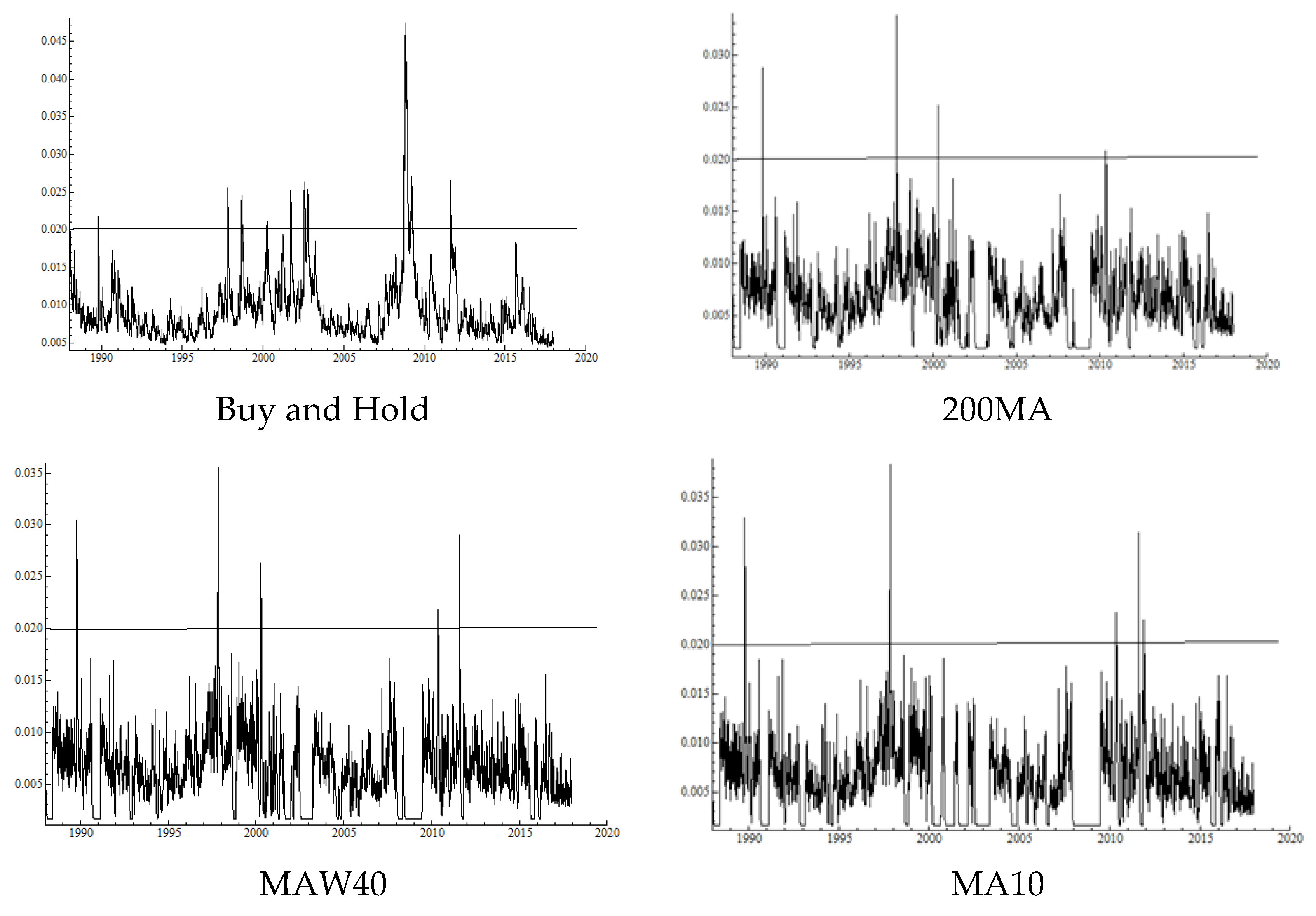
Table 1 presents the results where 200 trading days are used. We estimate conditional volatility on the basis of GARCH (1,1), reporting the average of yearly (1989–2017) estimated conditional volatilities for 260 trading days ahead, using the expanding window method. These estimates are also repeated for 400, 600 and 800 rolling windows returns. IGARCH processes are identified for almost all of the estimates.
The buy and hold strategy produces annualized returns before dividends of
+0.085 with the annualized volatility
0.167.
Table 1 shows that the annualized average volatility is
0.115 when MA rules are used, thereby reducing by about 31% compared with the buy and hold returns volatility. Note that
, and that the average US three month Treasury bill annualized yield has been
+0.022, indicating we invest
randomly 48% of time in the DJIA index from 4 January 1988, and 52% of time in the risk-free rate, thereby producing
+0.053 annually, on average, with
0.115 volatility.
Table 1 reports that, from the weekly frequency onwards, the MA rules exceed the random timing performance, before dividends. The average annualized dividends in the DJIA index have been
+0.026 for the last 30 years. Therefore, the Sharpe ratio of random market timing (48% in stocks and 52% in the risk-free rate), with dividends, is
0.38; for MA200, it is
0.32; for MAW40, it is
0.37; for MA10, it is
0.51; for MAD5, it is
0.47; for MAT4, it is
0.55; for MAQ3, it is
0.58; and for MAC2, it is
0.53.
We calculate the Sharpe ratio as follows:
where
is the annualized average returns for the trading rule
,
is the share of time invested in the stock index, 0.026 is the average annual dividend, 0.022 is the average annualized risk-free rate of return, and
is the annualized average standard deviation for the trading rule
. The annualized average standard deviation can be considered as an approximation for the unconditional volatility, where the GARCH effect is ignored.
However, the results with conditional volatilities are more drastic, that is, if the GARCH effect is taken into account. While the buy and hold strategy produces the average (estimated by each year) conditional volatility
0.255 a year ahead, the average MA trading rule volatility is reduced to
0.125, meaning a 51% reduction. When IGARCH is identified, the conditional volatility for 260 trading days ahead is given by:
where the
and
parameters are estimated using restricted GARCH (1,1),
is the return variance at time
, and
is the conditional variance at time
. We annualize this by multiplying the IGARCH result by
, and use robust standard errors for all the estimates at the 95% confidence level. The equation indicates that if
has a zero (positive) estimate, the IGARCH process forecast behaves as random walk without (with) drift.
Returns from 4 January 1988 to 29 December 1989 are the observations used for the first GARCH (1,1) estimates. Note that we approximate the conditional volatility of the random market timing 48% of the time, investing in stocks as follows:
. In addition,
Figure 1 shows the realized volatilities for these returns series.
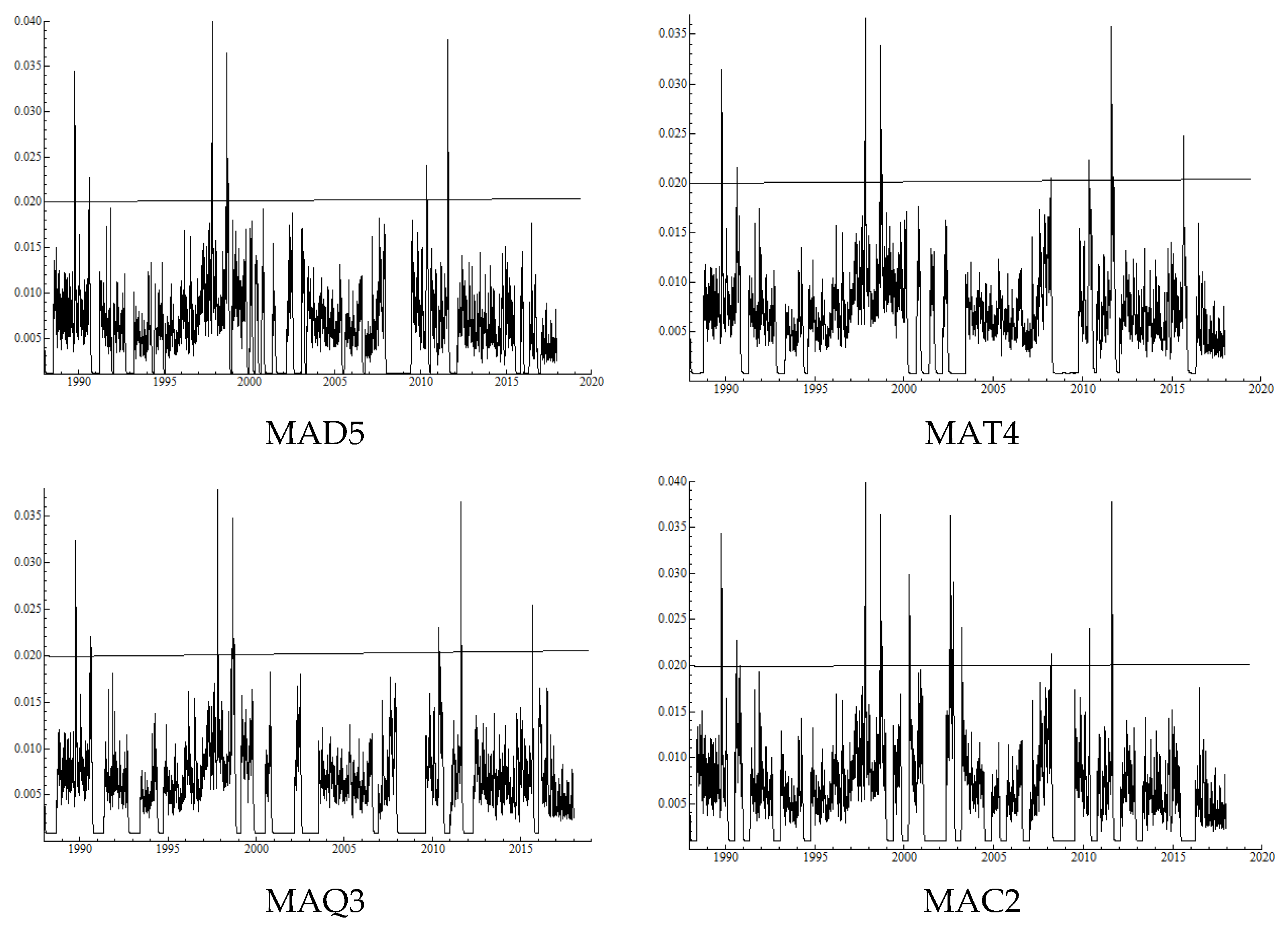
Table 2 shows that, with the 400 trading days rolling window, the annualized average volatility is
0.121, which means a reduction of 28% compared to the buy and hold strategy returns volatility when MA rules are used. This indicates in
random timing strategy that we invest (because
) 52% of the time in the DJIA index and 48% in the risk-free rate producing
+0.055 annually, on average, with
0.121 volatility. The Sharpe ratio of random market timing (52% in stocks and 48% in the risk-free rate) with dividends is
0.38; for MA400
0.38; for MAW80
0.46; for MA19
0.58; for MAD10
0.63; for MAT7
0.58; for MAQ5
0.55; and for MAC4
0.66.
The results concerning the conditional volatilities are again more drastic. While the buy and hold strategy produces average yearly conditional volatility for a year ahead 0.255, the trading rule volatility reduces to 0.098, on average, indicating a 62% reduction. Moreover, the conditional volatility for the random timing is approximated as:
.
Figure 2 shows the realized volatilities with these returns series.
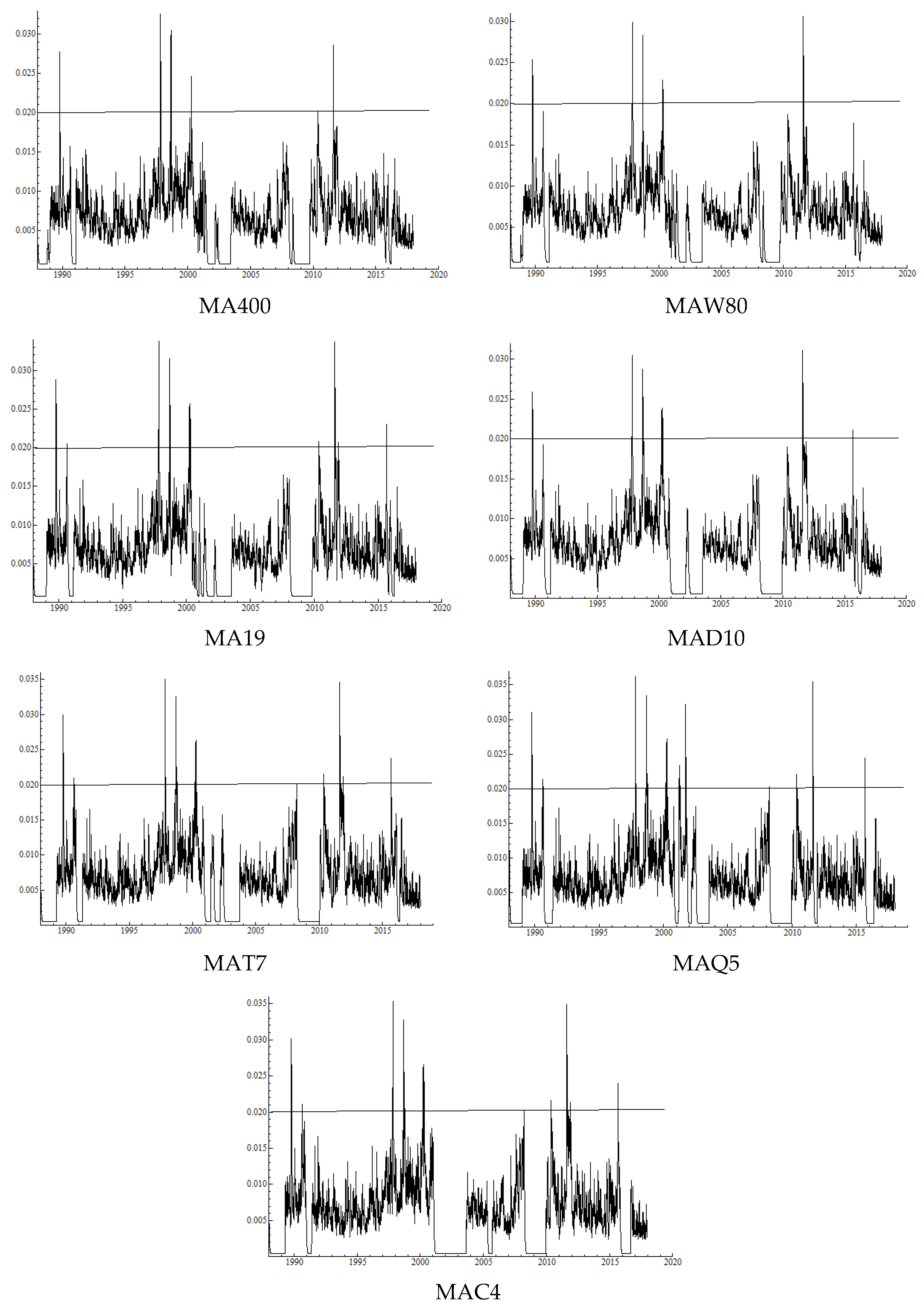
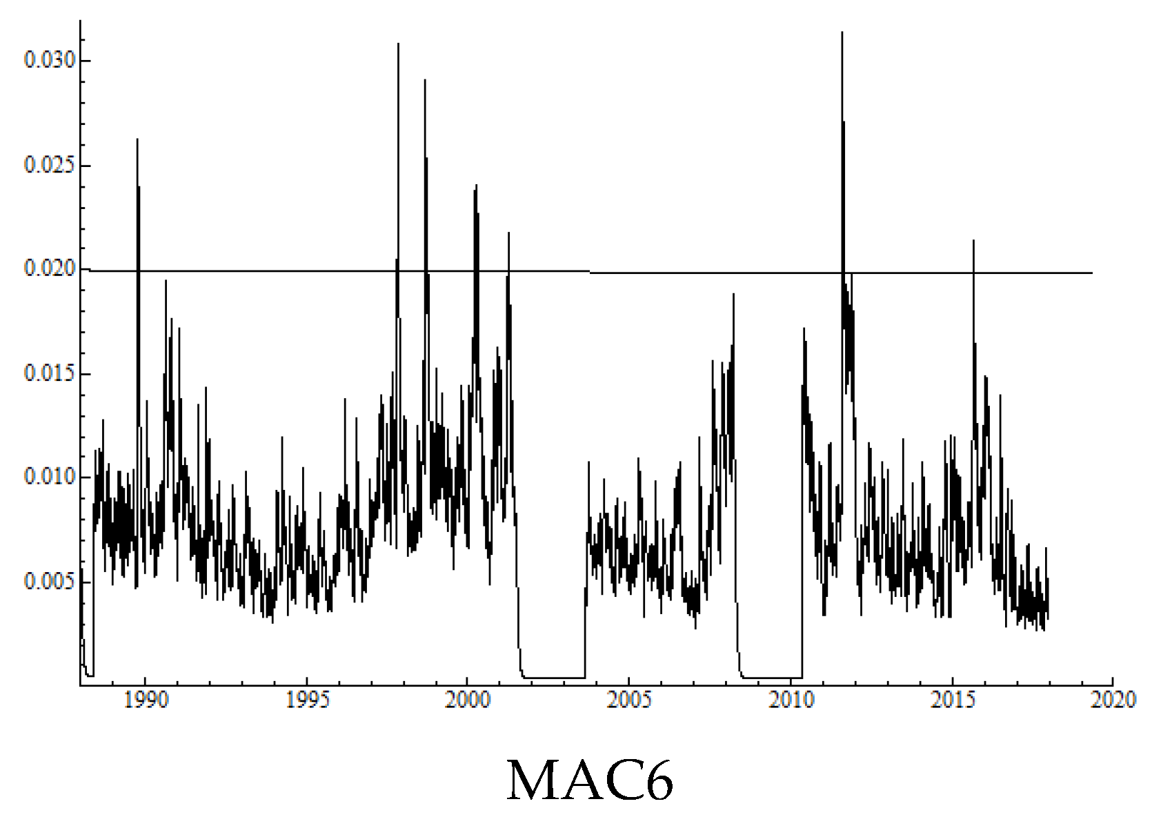
Table 3 shows that, with the 600 trading days rolling window, the annualized average volatility is
0.129, which means a reduction of about 23% compared with the buy and hold strategy returns volatility when MA rules are used. This indicates for the
random timing strategy that we invest 60% of the time in the index and 40% in the risk-free rate, producing
+0.060 annually before dividends, on average, with
0.129 volatility. The Sharpe ratio of random market timing (60% in stocks and 40% in the risk-free rate) with dividends is
0.42; for MA600, it is
0.55; for MAW121, it is
0.49; for MA29, it is
0.48; for MAD14, it is
0.50; for MAT10, it is
0.56; for MAQ7, it is
0.54; and for MAC6, it is
0.67.
The results regarding conditional volatilities are again more severe. While the buy and hold strategy produces the average conditional volatility for a year ahead 0.255, the trading rule volatility reduces to 0.158, on average, indicating a 38% reduction. The approximation for the random timing conditional volatility is
.
Figure 3 shows the realized volatilities with these returns series.
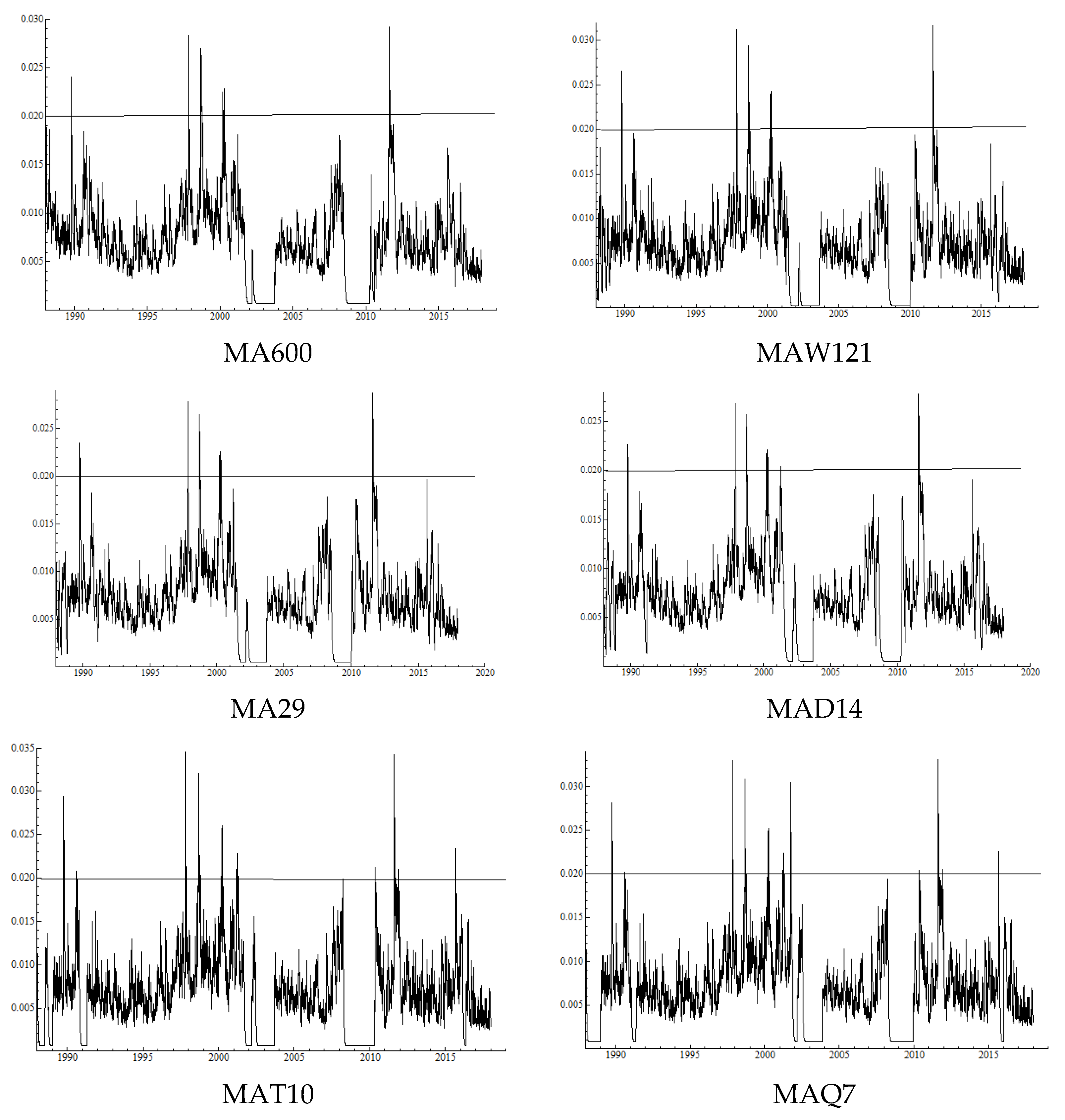
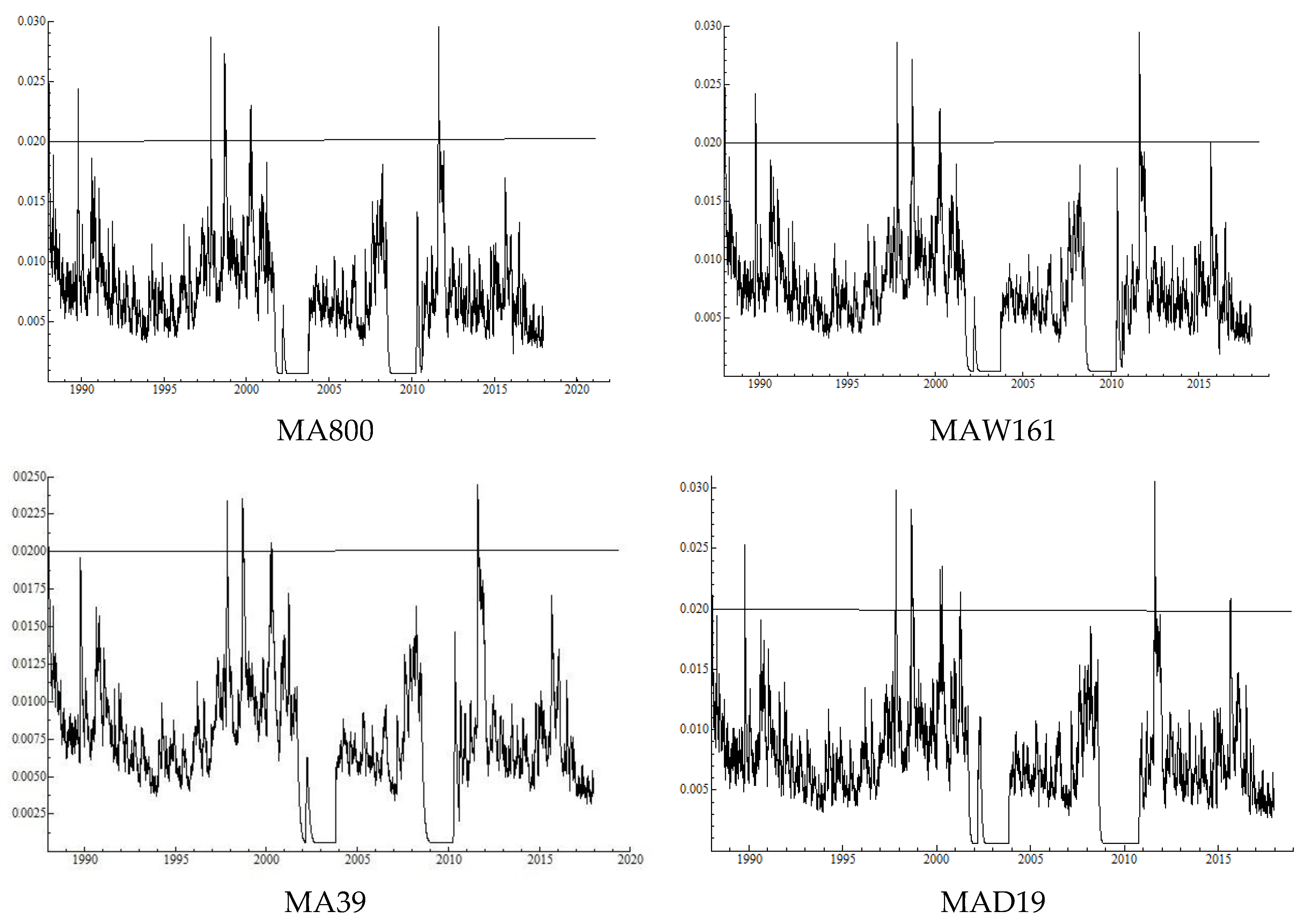
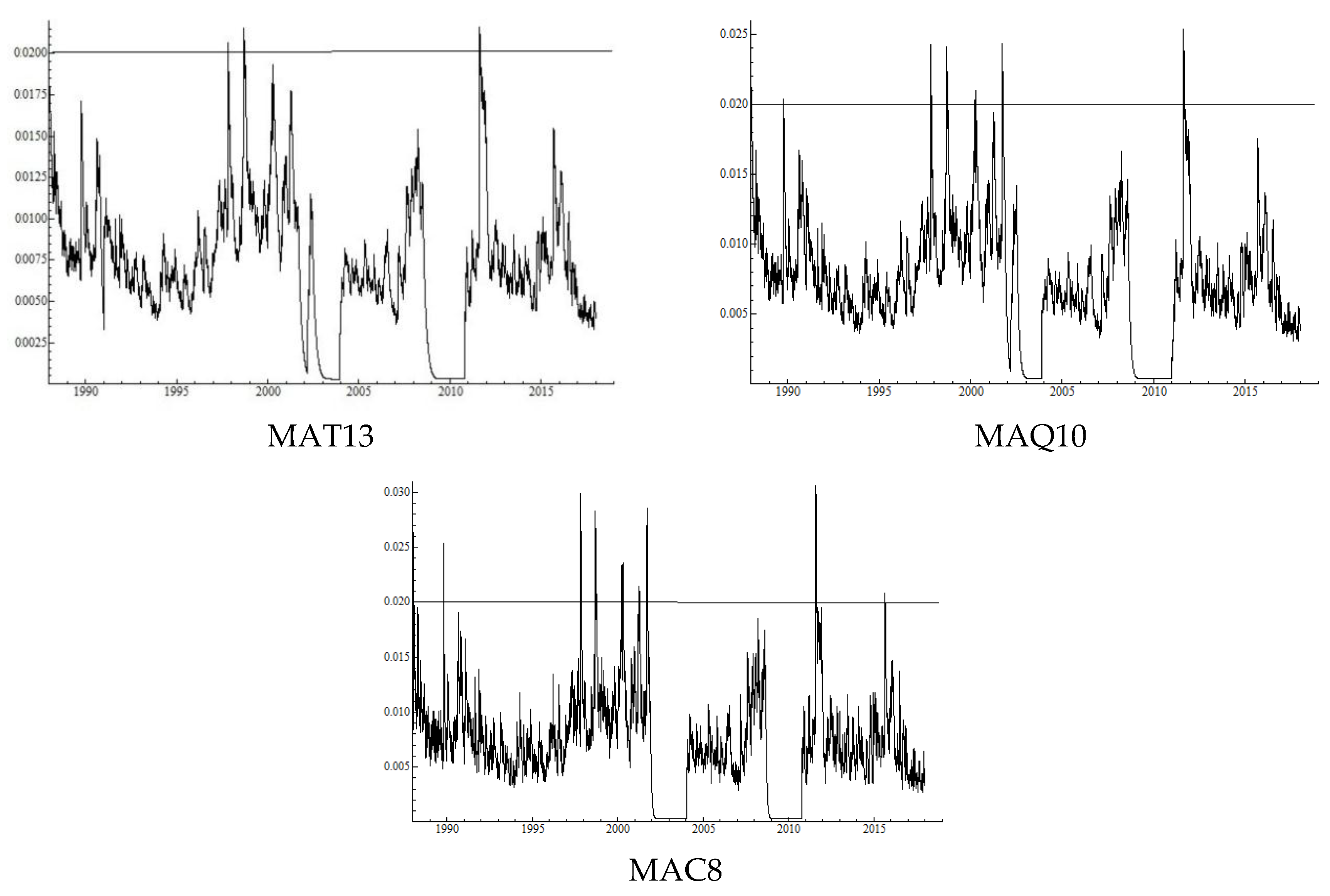
Table 4 shows that, with the 800 trading days rolling window, the annualized average volatility is
0.133, with a reduction of about 20% compared with the buy and hold strategy returns when MA rules are used. This indicates for the random timing strategy that we invest 64% of the time in the index and 36% in the risk-free rate, thereby producing
+0.062 annually before dividends, on average, with
0.133 volatility. The Sharpe ratio of random market timing (64% in stocks and 36% in the risk-free rate) with dividends is
0.43; for MA800, it is
0.58; for MAW161, it is
0.61; for MA39, it is
0.57; for MAD19, it is
0.60; for MAT13, it is
0.59; for MAQ10, it is
0.55; and for MAC8, it is
0.58.
Finally, the results using conditional volatilities are again more drastic. While the buy and hold strategy produces conditional volatility for a year ahead 0.255, the average trading rule volatility reduces to 0.148, on average, indicating a 42% reduction. Finally, the approximation for the random timing conditional volatility is
.
Figure 3 shows the realized volatilities with these returns series.
Table 5,
Table 6,
Table 7 and
Table 8 present rolling windows of 200, 400, 600 and 800 trading days, respectively, Sharpe ratios, data frequencies, and Sharpe ratios with conditional volatilities. The empirical results suggest that, when the size of the rolling window is 800 trading days (about three years), the significance of the frequencies in the MA rules becomes unimportant. In order to analyze how the size of the rolling window and the frequencies can affect the performance (see
Table 5,
Table 6,
Table 7 and
Table 8) in trading rules, we estimate the following regression models using Ordinary Least Squares (OLS):
where
denotes the Sharpe ratio,
denotes the rolling window, all explanatory variables are taken to be dummies, and the benchmark group is the random timing strategy. Therefore, Equations (2) and (3) contribute to the calculation of the analysis of variance (ANOVA).
In
Table 9 the Sharpe ratio and rolling window (RW) dummy variables are obtained from
Table 5,
Table 6,
Table 7 and
Table 8. HAC denotes the
Newey and West (
1987) Heteroskedasticity and AutoCorrelation (HAC) consistent standard errors. The empirical results show that three of the four estimated parameters are statistically significant, and the random timing strategy produces
0.40 for the Sharpe ratio, on average. With the rolling window of 200 trading days, the Sharpe remains the same statistically. However, RW400 produces
0.55, RW600 produces
0.54, and the rolling window of 800 trading days produces
0.58, on average.
Table 5,
Table 6,
Table 7 and
Table 8 show that the sample size is 32 for the OLS estimates in
Table 9,
Table 10,
Table 11 and
Table 12. According to the small sample adjusted Jarque-Bera test, the residuals are normally distributed, with a
p-value of 0.25. In view of the HAC consistent covariance matrix estimators, which are robust against alternative forms of misspecification in heteroscedasticity and autocorrelation, it is not necessary to provide further diagnostic checks.
These empirical results suggest that the widest window yields the best performance, beating the random timing performance by a 45% increase in the Sharpe ratio, on average. The adjusted R2 value is 0.34, indicating that the size of the rolling window explains about one-third of the variations in the Sharpe ratios. The empirical results show that even the stochastic trend information from three years ago seems to improve the performance of the trading strategies. Moreover, the random timing (efficient market hypothesis) performance is beaten by MA trading strategies, using the long run rolling window. This indicates that stock returns are more predictable in the long run.
Table 10 shows that five of the seven estimated parameters are statistically significant. Moreover, the random timing strategy produces a Sharpe ratio of
0.40, on average. However, using monthly frequencies, the Sharpe ratio increases to
0.54, every other month produces
0.55, every third month frequency produces
0.57, every fourth month produces
0.56, and every fifth month produces a Sharpe ratio of
0.61, on average. According to the small sample adjusted Jarque-Bera test, the residuals are normally distributed, with a
p-value of 0.78.
These results support the results of
Ilomäki et al. (
2018), suggesting that the lowest frequency produces the best performance, beating the random timing performance by a
51% increase in the Sharpe ratio, on average. The results suggest that using daily and weekly frequencies are practically useless, except when the widest rolling window is used. The adjusted
R2 value is
0.38, which indicates that the frequency explains 38% of the variations in the Sharpe ratios.
These empirical findings suggest that the long run stochastic trend information (that is, the observations in every fifth month), enhances the performance of trading strategies, and the random timing (efficient market hypothesis) performance is clearly beaten by MA trading strategies. This indicates that the stock returns are more predictable in the long run.
Next, we change the explained variable in Equations (2) and (3) to the Sharpe ratio, where the unconditional volatility is changed for the conditional volatility
measures in
Table 1,
Table 2,
Table 3 and
Table 4, and are presented in
Table 5,
Table 6,
Table 7 and
Table 8. We denote this performance measure as
, which is calculated as:
where
is the annualized average returns for trading rule
,
is the share of time invested in the stock index, 0.026 is the average annual dividend, 0.022 is the average annualized risk-free rate of return, and
is the annualized average conditional standard deviation, which is estimated yearly by GARCH(1,1) for 260 trading days ahead for trading rule
.
Then, we estimate the ANOVA equations:
where the benchmark group is the random market timing, and all the explanatory variables are taken to be dummies.
Table 11 presents the regression results for the model given in Equation (4).
Table 11 shows that all but one (RW200) of the estimated parameters are statistically significant, and the random timing strategy produces
0.26 for the
, on average. However, when the rolling window of 400 trading days is used, the
increases to
0.68, RW600 produces
0.50, and the rolling window of 800 trading days produces
0.53, on average. The small sample adjusted Jarque-Bera test shows that the residuals are normally distributed, with a
p-value of 0.48.
The empirical results show that three of the four estimated parameters are statistically significant, and suggest that RW400 (a year and a half) yields the best performance, beating the random timing performance by a 158% increase in , on average. The adjusted R2 value is 0.31, indicating that the size of the rolling window explains about one-third of the variations in the . However, the empirical findings suggest that even the stochastic trend information from three years ago seems to improve the statistical performance of the trading strategies. Moreover, the random timing (efficient market hypothesis) performance is beaten by MA trading strategies, with the long run rolling window increasing by 100%. This outcome indicates that the stock returns are indeed predictable in the long run.
Table 12 presents the regression results for the model given in Equation (4), in which all seven estimated parameters are statistically significant. The table shows that the random timing strategy produces
of
0.26, on average. However, with daily, weekly, and monthly frequencies, the
does not increase significantly (at the 5% level of significance). On the other hand, every other month produces
0.51, every third month frequency produces
0.62, every fourth month produces
0.72, and every fifth month produces a Sharpe ratio of
0.64, on average. The small sample adjusted Jarque-Bera test shows that the residuals are normally distributed, with a
p-value of 0.72. The realized volatilities for the 800 trading days rolling window are given in
Figure 4.
These empirical results suggest that every fourth month frequency produces the best performance, beating the random timing performance by an increase of 173% in the , on average. The adjusted R2 value is 0.38, indicating that the frequency explains 38% of the variations in the Sharpe ratios when the conditional volatilities are accommodated.
5. Conclusions
This paper investigated the performance of moving average (MA) market timing strategies when the rolling window used in such strategies was expanded, and the frequency used in the calculations was also changed. The timing considered 200, 400, 600 and 800 trading days rolling windows, and daily, weekly, monthly, every other month, every third month, every fourth month, and every fifth month frequencies were used. The primary purpose is to apply MA rule returns performance as an instrument for testing returns predictability in stock markets.
The first empirical finding is that, on average, using daily or weekly frequencies does not beat random market timing performance. For example, the MA200 trading rule, which is the most common rule among practitioners, underperforms the random market timing strategy. However, it was also found that, when the rolling window was expanded from 400 trading days (a year and a half) onwards, with monthly and lower frequencies, the performance of MA trading strategies started to exceed that of random market timing when the unconditional volatility was used in the Sharpe ratios. Random market timing dominates if expected stock returns were constant or, as in our test, if the Sharpe ratios with unconditional and conditional volatility were fairly constant over time.
Furthermore, we found that, when the unconditional volatility was changed to the conditional volatility in the Sharpe ratios, the results became more variable, as expected, but the main results remained fairly consistent with each other. However, when the conditional volatility was incorporated in the Sharpe ratio, then the monthly frequency seemed to lose power in predicting stock returns, on average. In addition, when the size of the rolling window reached 800 trading days (about three years), the frequencies produced a similar performance in the tested MA rules. This included both Sharpe ratios using unconditional and conditional volatilities.
In summary, the empirical results indicated that stock returns were indeed predictable in the long run, and also over business cycles and stochastic trends. The results were also independent of the persistence issues of explanatory variables in predictions, which have been noted in the literature, because only returns were considered in the empirical analysis.


