1. Introduction
Decentralized finance (DeFi) has emerged as a transformative paradigm within the financial landscape, harnessing the capabilities of blockchain technology to reshape traditional financial services. As the DeFi space continues to evolve rapidly, there is a growing need to comprehensively understand and assess the performance of these protocols in dynamic and unpredictable market conditions.
In a space where innovation and experimentation abound, the ability to simulate and analyze the behavior of DeFi protocols becomes paramount for both developers and participants. One of the key challenges lies in predicting how these protocols will perform under varying market scenarios, which are inherently influenced by the volatile nature of the cryptocurrency market.
Against the backdrop of dynamic cryptocurrency trading, a myriad of platforms has mushroomed globally, each contributing to the evolving narrative of DeFi. These platforms, while presenting distinct advantages and limitations, share a common thread: the direct connection of economic entities for mutual gains in cryptocurrency trading.
Prominent actors in the DeFi lending space include Uniswap, Sushiswap, Compound, and Aave. Despite their progress, challenges persist, ranging from scalability issues, to elevated transaction costs and barriers, and the seamless onboarding of new users. The current state of research in DeFi lending protocols reflects a robust exploration of facets such as smart contract architecture, token mechanics, governance models, and user behavior.
Uniswap, operating on the Ethereum blockchain, utilizes an Automated Market Maker (AMM) model, promoting trustless and permissionless token trading. Researchers (
Adams et al. 2021;
Angeris et al. 2019;
Daian et al. 2019) have scrutinized its pricing mechanism, liquidity provision strategy, security vulnerabilities, and optimization strategies.
Sushiswap, born as a decentralized exchange (DEX) and AMM, distinguishes itself by amplifying liquidity and incentives for liquidity providers (LPs). Research (
Fan et al. 2023) undertakings delve into the intricacies of liquidity mining incentives, the sway of economic factors on liquidity providers’ decision making, and strategies to alleviate impermanent loss.
Compound, a decentralized lending protocol, revolutionizes DeFi by enabling users to lend or borrow based on algorithmic interest rates. Researchers (
Saengchote 2023;
Kao et al. 2020) have evaluated its market risks, liquidation mechanism, and economic security through agent-based modeling and simulation.
Furthermore, a nuanced exploration branches into the broader financial ecosystem, with a focus on three prominent Peer-to-Liquid Funds (PLFs)—Aave, dYdX, and Compound, presented in (
Gudgeon et al. 2020). Market liquidity, efficiency, and interdependence among these PLFs take center stage, unraveling operational patterns during periods of high utilization and the potential risks associated with liquidity concentration.
Aave, akin to Compound, stands as a decentralized lending and borrowing platform with a distinctive feature—flash loans. The founder’s whitepaper (
Aave n.d.) provides a comprehensive elucidation of Aave’s innovative lending pool model, flash loans, and governance structure. The research (
Sun et al. 2023) threads weave through topics such as risk management, interest rate models, and liquidity provision, offering valuable insights into the multifaceted dynamics of the Aave protocol.
The cryptocurrency market is renowned for its inherent volatility, characterized by rapid and sometimes unpredictable price fluctuations across various digital assets. This volatility is a key distinguishing feature of the crypto market and is influenced by a myriad of factors. In (
Gupta and Chaudhary 2022), the authors empirically found that there is the presence of high volatility among the returns of four cryptocurrencies—Bitcoin, Ether, Litecoin, and XRP—which makes them very risky assets for investments.
One of the primary contributors to cryptocurrency market volatility is the market’s relative nascency. Compared to traditional financial markets, the crypto space is relatively young and less mature. As a result, it tends to be more susceptible to sudden market sentiment shifts, speculative trading, and external influences. In a period where positive sentiment regarding the adoption of cryptocurrencies becomes widespread, financial institutions and large corporations increasingly integrate cryptocurrencies into their operations and investment portfolios. Increased adoption by traditional financial players can significantly boost the credibility and acceptance of DeFi platforms. Positive market sentiment often correlates with increased demand and can positively influence the valuation of cryptocurrencies.
Other factors affecting the volatility of cryptocurrencies are the regulatory developments. A global push among major economies for clearer and more favorable cryptocurrency regulations may introduce regulatory frameworks that legitimize and provide clear guidelines for the operation of decentralized finance (DeFi) platforms. This regulatory clarity could positively impact investor confidence, potentially leading to increased participation in platforms such as NOLUS. Conversely, adverse regulatory developments could introduce uncertainty and hinder growth.
The decentralized nature of many cryptocurrencies also plays a role. Without a central governing authority, market movements can be more reactive to news, social media trends, or macroeconomic factors. In terms of a global economic downturn, traditional financial markets experience a recession, and central banks implement expansive monetary policies to counter economic challenges. Economic downturns might drive investors toward alternative assets, including cryptocurrencies, as a hedge against economic uncertainties. This shift could influence the demand for cryptocurrencies and impact their pricing dynamics.
Liquidity, or the ease with which an asset can be bought or sold, is another factor amplifying crypto market volatility. Low liquidity in certain markets can result in larger price swings, as a relatively small volume of trades can have a significant impact.
Moreover, significant technological advancements in blockchain and decentralized technologies also affect the volatility of crypto markets. This could include the widespread adoption of more efficient consensus algorithms, scalability solutions, or interoperability protocols. Technological progress can enhance the efficiency and functionality of DeFi platforms. If these platforms integrate these advancements, they might gain a competitive edge, attracting more users and positively affecting their valuation.
In recent years, the crypto market has witnessed efforts to mitigate volatility. The introduction of stablecoins pegged to traditional fiat currencies, algorithmic stablecoins, and decentralized finance (DeFi) protocols seeking to stabilize token values are examples of such endeavors. However, volatility remains a characteristic element of the crypto landscape, offering both opportunities and challenges for investors and traders.
The novelty of our approach rests on the integration of historical crypto market data into the simulation of a newly developed protocol performance. By leveraging past market behaviors, we create a realistic environment that captures the complexities of real-world conditions, enabling us to evaluate the performance, risks, and potential outcomes of the real protocol with greater precision.
The subsequent sections of this paper focus on the details of our simulation methodology, the data sources and variables used, and the results of our analyses. Through researching the dynamic performance of the presented protocol using historical market simulations, we contribute to the ongoing discourse surrounding the evolution of DeFi, its potential challenges, and the opportunities it presents within the ever-evolving landscape of decentralized finance.
The
Supplementary Materials section of the article provides an address that directs to the repository where the actual model of the real platform is published. This facilitates the ability of other researchers to replicate and build upon the presented results.
2. Mechanisms for Implementation of a DeFi Protocol Simulation
2.1. Event: Interest Generation
2.1.1. Lessees Interest (LS Interest)
The interest rate definition plays a crucial role in DeFi protocols as it directly impacts the functioning and effectiveness of these platforms. The accurate and well-defined determination of interest rates is essential for maintaining stability, attracting users, and ensuring efficient capital allocation within the DeFi ecosystem.
One of the key aspects of DeFi protocols is lending and borrowing activities, where users provide or borrow funds from the platform. The interest rate serves as a fundamental mechanism for incentivizing participation, balancing supply and demand, and managing risk.
A clear and transparent interest rate definition is important for several reasons. Firstly, it ensures fairness and equal treatment of all participants. By having a standardized and objective method of calculating interest rates, users can trust that their loans or deposits are subject to consistent and predictable terms.
Secondly, the interest rate definition helps to maintain stability and mitigate risks within the DeFi ecosystem. Through careful consideration of market conditions, collateralization ratios, and other factors, protocols can establish interest rates that align with the underlying assets’ risk profiles. This helps to protect the platform and its users from excessive volatility and potential defaults.
Moreover, the interest rate definition enables efficient capital allocation by incentivizing borrowing or lending activities when they are most needed. By dynamically adjusting interest rates based on supply and demand dynamics, protocols can influence user behavior and optimize resource allocation.
Furthermore, the interest rate definition in DeFi protocols is an area of active research and innovation. It involves considerations of economic theories, game theory, and algorithmic mechanisms. Researchers and developers are constantly exploring novel approaches to improve interest rate models, liquidity provision, and risk management to enhance the overall efficiency and sustainability of DeFi platforms. In (
Gudgeon et al. 2020), the authors presented evidence of the inefficiency of DeFi tokens regarding their liquidity, market efficiency, and interest rates. They investigate the mechanisms used to set the interest rates in several DeFi protocols in order to find how to equilibrate the supply and demand for funds.
In (
Piñeiro-Chousa et al. 2022), the authors investigate the impact of certain traditional assets on specific DeFi tokens, focusing on their volatility. The study suggests that there are connections between traditional assets, user-generated content, and DeFi tokens. These relationships indicate that DeFi tokens may serve as safe havens and provide a hedge against stock market volatility.
The value of LS Interest due on the smart contracts in the NOLUS platform is calculated daily and it consists of two components: a predefined Base Interest Rate and an additional part dependent on the Utilization Rate of the relevant pool.
The first component—the Base Interest Rate—is set for the platform and it serves as a minimum return that is guaranteed throughout the entire duration of the smart contract, except for the cases in which conditions for liquidation occur.
The second component—the Utilization Rate—is calculated daily from the ratio between the total amount of assets in stable currency already borrowed from the respective pool and the value of the deposited amounts in stable together with the accumulated interest in stable. It represents the part of the assets from each pool that are borrowed from the LSs.
For calculation of the Utilization Rate on a daily basis for every pool, the following formula is used:
where
- -
—Utilization Rate per pool;
- -
—the total amount borrowed from the pool’s native asset in stable for a specified timestamp;
- -
—the Total Value Locked (TVL) amount of the pool’s native asset in stable for a specified time.
The TVL is further discussed in
Section 2.3 of this article.
At the end of each day, when the smart contracts are closed, the Utilization Rate for each pool is calculated, and the following day, this Utilization Rate is taken for calculation of the LS interest rate for the current day.
In case at any day a 100% Utilization Rate is reached for a specific pool, no contracts are opened on that day and the day is restarted.
The interest rate for each individual pool, which represents the interest rate for the LS contracts, is calculated as per the formulas below, according to the level of utilization of the respective pool:
- (1)
when the Utilization Rate for the pool is smaller than or equal to the Optimal Utilization Rate, i.e.,
:
- (2)
when the Utilization Rate for the pool is higher than the Optimal Utilization Rate, i.e.,
:
where
- -
—a variable interest rate per pool;
- -
—a predefined Base Interest Rate;
- -
—the Utilization Rate;
- -
—a predefined Optimal Utilization Rate for the stable pool;
- -
—a predefined parameter, showing the increasing of the interest rate when ;
- -
—a predefined parameter, showing the increasing of the interest rate when .
This approach can be found also in the Aave protocol (
Aave n.d.).
2.1.2. LP Interest
When a new liquidity provider (LP) deposit is opened, the amount of the deposit is stored both as an asset and is recalculated in stablecoins. The LP interest rate for a particular timestamp is calculated on a daily basis for each separate pool, according to the formula:
where
- -
—the LP interest rate for a particular timestamp;
- -
—a variable interest rate per pool for a particular timestamp;
- -
—a predefined Treasury Interest Rate.
At the time of withdrawal of the deposit from the LP, the cumulative amount of each LP’s interest is paid to them, together with the amount of their deposit and the additional profit in the form of NOLUS tokens (NLSs).
An important point to mention is a specific characteristic of the platform, regarding the number of LS contracts that will be opened daily, in reference to the change in the interest rate. The number of newly opened LS contracts depends on the interest rate and the Utilization Rate for the particular day.
The number of LS contracts that will be opened for the respective day decreases when the interest rate increases.
This functionality is achieved using the following formula:
where
- -
—percentage demand;
- -
—minimal LS interest;
- -
—maximal LS interest;
- -
—the maximum value of the variation in the parameter demand when forming the corresponding structure;
- -
—the minimum value of the variation in the parameter demand when forming the corresponding structure.
It is foreseen that there is a predefined maximum allowed LS interest rate. The parameter “dem” is calculated, which shows the percentage of the contracts for the corresponding day that will be opened depending on the interest rate calculated for the particular day. This functionality demonstrates that the interest of the LSs can decrease depending on the increase in the interest rates for the new contracts.
The maximum Pool Utilization, predefined in the config file, is used for LS demand reduction. If the maximum Pool Utilization is reached, the staked daily counts of new contracts are multiplied by weight for the purpose of reduction.
2.2. Event: Repayment of Loans by LSs
In the context of smart contracts, repayment refers to the process of returning borrowed assets to the lending platform after a borrower has completed their loan term.
In (
Carapella et al. 2022), the authors provide an overview of blockchain basics and the major DeFi protocols and products they offer, together with the mechanisms for repayment of smart contracts, and finally they cover potential risks associated with these technologies and use cases. In (
Gudgeon et al. 2020), the authors conduct an empirical analysis to observe the behavior of interest rate rules since their introduction, focusing on their responses to various levels of liquidity.
There are three types of liquidation transactions in NOLUS protocol, regarding the payment of loans by the LSs:
- -
Regular payment or liquidation due to penalty;
- -
Partial liquidation;
- -
Total liquidation.
The first type of liquidation refers to the regular payments made by the LSs to repay their obligations under the smart contracts. These regular payments are executed without the need for manual intervention once the smart contract has been deployed on the blockchain. Regular payments in smart contracts provide several advantages, including reducing administrative overhead, enhancing trust and transparency, and ensuring timely and accurate payments.
The partial liquidation mechanism is crucial for maintaining the stability and safety of the protocol. It helps protect lenders and maintain the overall health of the system by preventing excessive losses in the event of volatile market conditions or borrower defaults. Partial liquidation refers to the reduction in a given asset of the LS as a result of one of the following two events: omitted payments or a shake-up in market conditions. When partial liquidation occurs, the smart contract will automatically sell or auction off a portion of the user’s collateral to cover their outstanding debt and ensure that the protocol remains solvent. By liquidating only a part of the collateral, users have the opportunity to restore their position and prevent the complete loss of their assets.
Full liquidation refers to the process of completely liquidating a user’s collateral in the smart contract when they are unable to meet their debt obligations or the value of their collateral falls below a critical threshold. Full liquidation is an essential risk management mechanism in the protocol, as it helps to mitigate the impact of defaulting borrowers and ensures the stability and security of the system. By fully liquidating a user’s collateral, the protocol can recover the debt owed and maintain the integrity of its reserve funds, which are critical for providing liquidity and maintaining the overall health of the platform.
There are some assumptions regarding the liquidation of contracts in the NOLUS platform that should be mentioned, as follows:
where:
- -
—the value of the LSs loan (loan amount) at the conclusion of the contract in asset;
- -
—the collateral (downpayment) in asset provided by LSs upon conclusion of the smart contract;
- -
—the borrowed amount of asset from the LSs.
- -
—the value of the LSs loan at a given time in stable;
- -
—the market price of the particular asset for the current timestamp.
All obligations due on the contract at a given time in stable,
, can be calculated as follows:
where
- -
—all obligations due on the contract at a given time in stable;
- -
—the principal due on the LS contract at a given time in stable;
- -
—the LS interest due on the contract at a given time in stable.
In turn, the following formula is used to determine the
:
where
- -
—the market price of the relevant asset at the time of opening the smart contract;
- -
—the already paid part of the principal.
The value of
indicates the current interest standing at any given time. In the Monte Carlo simulation, the interest is used as the standing interest for the next month (example: when a contract is opened initially,
is set as the value of the interest for 1 month).
where:
- -
—Lease Liability: ratio between borrowed to collateral at a given time.
There are three parameters, regarding the Lease Liability:
- -
—Lease Initial Liability: a predefined initial Lease Liability in %;
- -
—Lease Healthy Liability: a predefined healthy Lease Liability in %;
- -
—Lease Max Liability: a predefined maximum Lease Liability in %.
It is foreseen that the for every opened contract is recalculated daily. The of the contracts should be smaller than or equal to , and is smaller than , to ensure that the protocol will work optimally and that no shortage of funds will occur in the pools.
2.2.1. Liquidation Type 1: Regular Payment/Liquidation Due to Penalty
It is expected that in the majority of cases, the contracts in the platform will be paid out in a timely manner; hence, there will be no penalty payments. In these cases, for the regular repayment of every smart contract, the following formula is used:
where
- -
—the amount of the regular payment (repayment amount);
- -
—the principal of the contract together with the newly achieved asset in stable;
- -
—the number of regular payments under the contract (payment);
- -
—the number of omitted payments under the contract (penalty).
For calculation of the omitted payments the following formula is used:
where
- -
—the amount of the omitted (penalty) payment.
As mentioned, there are two conditions for a partial or a full liquidation to occur: missed contract payments or market shocks. When any of these events occurs and a set depreciation threshold is reached, part of the LS’s asset is sold in order to bring it to a sustainable state.
At the opening of the contracts for the current day, for each contract is calculated and the following rule applies:
If ≥ , it indicates that ≥ ; then, the liquidation amount in stable at the current moment ( is calculated and the amount is stored in a specific structure of the protocol.
The following formula is used to define
and the smaller of the following two values is taken:
where
- -
—liquidation amount for a given time in stable: the amount in stable by which the should be reduced after the partial liquidation for the current time.
2.2.2. Liquidation Type 2: Full Liquidation
If , then a full liquidation is enforced.
After all liquidations past time for the totally liquidated contracts are removed, a liquidation record is created and a closing record for each fully liquidated contract is created.
2.2.3. Liquidation Type 3: Partial Liquidation
If , then a partial liquidation is enforced.
after the partial liquidation is calculated as follows:
After that, , representing the current interest standing at any given time, is also reduced in compliance with the new parameters of the smart contract.
2.3. Event: Total Value Locked
Total Value Locked is a crucial metric in the decentralized finance (DeFi) ecosystem, representing the total amount of assets locked in a specific protocol or across multiple protocols. It provides valuable insights into the protocol’s performance and helps investors, users, and the wider community make informed decisions in the rapidly evolving DeFi landscape. According to the empirical evidence presented by (
Maouchi et al. 2022), TVL can be used to evaluate DeFi tokens and monitor the market, and can be used as an indicator of the growth and success of that market (
Şoiman et al. 2022).
In (
Saengchote 2021), the author provides insights into the potential significance of TVL in DeFi and emphasizes the intricate nature of DeFi analysis and market monitoring. The author highlights that TVL is determined by the market value of tokens that are deposited or locked within the system, which inherently makes it sensitive to token prices. Consequently, there is an anticipated notable correlation between this variable and valuations. The study of (
Metelski and Sobieraj 2022) aims to assess key DeFi performance metrics, particularly focusing on protocol valuations. Through a quantitative analysis of 30 selected protocols across decentralized exchanges, lending, and asset management classes, the research explores relationships between protocol valuations and variables such as Total Value Locked (TVL), protocol revenue, total revenue, gross merchandise volume, and the inflation factor. Utilizing Granger causality tests and fixed effects panel regression models, the study reveals that DeFi protocol valuations exhibit dependencies on various performance measures, with distinct magnitudes and directions for different variables.
The significance of TVL can be found in several directions:
Measure of protocol adoption: TVL provides a measure of the level of adoption and acceptance of a DeFi protocol. A higher TVL indicates that more users are trusting and utilize the protocol to lock their assets, which demonstrates confidence in its security, functionality, and potential returns.
Indicator of liquidity: TVL serves as an indicator of the liquidity available within a protocol. Higher TVL implies a deeper pool of assets, which enhances trading efficiency, reduces slippage, and attracts more participants to engage in transactions.
Market perception and reputation: TVL plays a role in shaping the market perception and reputation of the DeFi protocol. A protocol with a substantial TVL is often seen as more reputable, reliable, and trustworthy by users, investors, and the wider DeFi community. This can attract further adoption and partnerships, enhancing the protocol’s long-term sustainability.
Comparative analysis: TVL allows for comparative analysis among different DeFi protocols. By assessing TVL across various platforms, investors and users can evaluate the relative popularity and growth potential of protocols, aiding in investment decision making and identifying emerging trends in the DeFi space.
Protocol governance and influence: TVL often influences the governance power within a DeFi protocol. Some protocols allocate voting power based on the amount of assets locked, giving higher TVL participants a stronger voice in decision-making processes. This aligns the interests of token holders with the protocol’s development and ensures the protocol evolves in a way that benefits the majority of participants.
The definition of TVL in the protocol is the following:
where
- -
—the cumulative deposited amount in the platform for the current time in stable;
- -
—the total amount of withdrawals of LPs from the platform for the current time, together with the corresponding LP interest;
- -
—the accumulated interest from LSs in the platform for the current time.
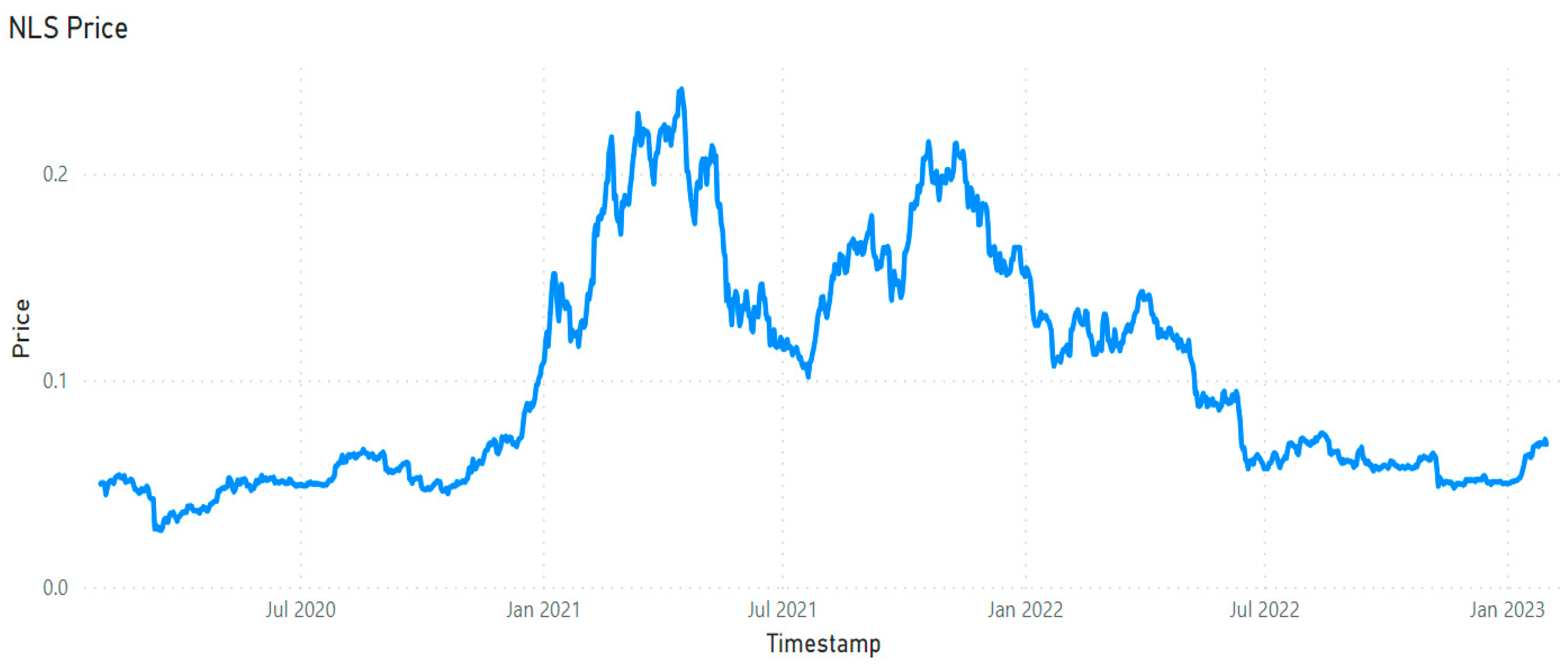
2.4. Event: NLS Price Definition
The price of the NLS tokens should be simulated as there is no historical information. It is formed of two components: the market price of the NLS and the impact of the protocol’s performance on the price. These two components are taken in a specified proportion and the final price of NLS is calculated.
The first component is a representation of the historical price of the currencies that participate in the platform, taken in a specific proportion.
The second component that participates in the formation of the final price of NLS tokens is the work of the protocol itself. To determine the influence of the platform on the level of the price of NLS tokens, the Total Value Locked is used.
This process is implemented in the following steps:
The ratio between the current value of all assets locked in the platform, calculated in stablecoins, and the total value of assets from the previous moment, is determined as follows:
- -
—the TVL of the pool’s native asset, calculated in stable for a specific time;
- -
—the TVL of the pool’s native asset, calculated in stable for a previous time.
- 2.
The proportion in which the two components will participate in forming the final price of the currency is determined.
- 3.
The final price, taking into account both the market price and the impact of the platform over the price of the NOLUS tokens, is calculated according to the formula:
where
- -
—the price of NLS tokens for the current timestamp;
- -
—the market price of NLS tokens;
- -
—the weight of the market price;
- -
(1 − )—the weight of the platform;
- -
—the price of NLS tokens for the previous timestamp.
2.5. LP Rewards Distribution
The Treasury is a part of the protocol where the profit from the work of the protocol is stored. In the beginning it is provided that there is an initial investment in the Treasury in the form of NLS tokens, which will ensure the necessity of having some funds in case any LP withdraws their deposit earlier, when the profit of the Treasury is not enough.
There are three cash inflows into the Treasury:
For the purposes of the simulation of the protocol, it is assumed that each LS and LP will pay a predefined number of transactions every month, so the total value of all transaction fees for the platform per month is calculated as follows:
where
- -
TRNF—total transaction fees;
- -
—the number of transactions made by each LS per month, predefined in the config file;
- -
—the number of transactions made by each LP per month, predefined in the config file;
- -
—the number of opened LS contracts per month;
- -
—the number of opened LP deposits per month;
- -
—the transaction price for each transaction in stable, predefined in the config file.
- 2.
SWAP fees—a one-time fee paid by each LS upon conclusion of the smart contract, predefined in the config file as a percent from the LS loan amount in stable:
where
- -
—LS loan amount in stable at the opening of the contract;
- -
—a predefined percent in the config.
- 3.
Treasury interest (TRI)—A predefined part of the interest paid by LSs
The cash outflow from the Treasury, which leads to a decrease in the accumulated funds in the Treasury, is the distribution of rewards to the LPs. These rewards are distributed among all LPs based on their percentage contribution to the pools on a daily basis.
The total amount of rewards per pool that are distributed among all LPs for a particular pool daily due to the initially deposited amount by each LP is calculated as follows:
where
- -
—Treasury rewards: the total amount of rewards per pool distributed among all LPs on a daily basis;
- -
trw—preliminary defined percentages of rewards per pool;
- -
—TVL per pool at the current time of the spread.
trw represents preliminary defined percentages that determine the relationship between the amount of TVL for all pools and the percentage of rewards for LPs. This relationship indicates the percentage of the TVL that will be distributed among the LPs. This value is extracted from the available funds in the Treasury and used for buyback of NLS tokens that will be spread among the LPs through rewards.
The rewards that each LP will receive from the Treasury daily are calculated as a percentage of all rewards that will be distributed among all LPs from the respective pool for the current day. This percentage depends on the amount of the deposit with which the respective LP participates in the specific pool, relative to the total deposited amount of all contracts for the current time for the pool in stable. After the individual percent for each LP is calculated, the amount of the rewards for the current day for each LP is determined.
In this way, the total cash inflow and outflow from the work of the protocol is stored in the Treasury and can be represented as follows:
where
- -
—Treasury profit, being the amount entered in the Treasury on a daily basis in stable;
- -
—total transaction fees on a daily basis in stable;
- -
—SWAP fees on a daily basis in stable;
- -
—the Treasury interest on a daily basis in stable;
- -
—Treasury rewards in stable that should be distributed among all LPs on a daily basis in stable.
The current state of the Treasury is recorded in stable in a specific structure, namely, NLS, which appears to be a cumulative table indicating the available funds in the Treasury at the current time, according to the following formula:
An important feature of the platform, related to the distribution of rewards to the LPs from the protocol, is the established mechanism, which ensures that, if for a specific day there is not a sufficient number of tokens in the Treasury to be distributed among all LPs, then for the corresponding day no rewards are distributed.
4. Conclusions
In conclusion, the simulation of the NOLUS protocol presented in this paper marks a significant stride toward comprehending the intricate interplay between decentralized finance protocols and the broader crypto market landscape. By harnessing historical crypto market data, we have effectively simulated the dynamic behavior of the NOLUS protocol.
The article explores several prominent DeFi protocols within the broader cryptocurrency market, with a specific focus on comparing the NOLUS platform, introduced in the article, to these established protocols. It provides an elaborate description of the developed software model that mimics the real protocol, delving into the core dependencies among its components. The article thoroughly examines the fundamental interdependencies among the various elements constituting the NOLUS protocol. Through a series of carefully conducted experiments, the platform’s functionality is scrutinized, utilizing predetermined values for numerous simulation parameters. The outcomes of these experiments affirm that the constructed model effectively mirrors the intricacies of the actual platform, presenting a highly accurate representation.
This simulation methodology has the potential to uncover critical protocol behaviors caused by potential crypto market dynamics, identify optimization opportunities, and highlight best practices for adjustment of the key protocol hyper parameters. As the DeFi ecosystem continues to evolve, these insights will prove instrumental in fostering a robust and sustainable DeFi landscape.
The simulation presented in this article is a one-time implementation of the actual DeFi platform NOLUS. As it involves numerous random factors and is based on certain assumptions about their distribution, this singular simulation is constrained by the initial hypotheses. Concurrently, historical cryptocurrency price data spanning three years was employed to replicate the platform’s behavior, intending to illustrate its hypothetical performance over that period. Recognizing these constraints, it is important to note that a detailed simulation of every operational aspect of the real platform might not be feasible. However, utilizing the developed model, which encapsulates the platform’s embedded mechanisms, and conducting multiple simulations, could facilitate a more profound analysis of the protocol.
The implications of this research extend beyond the immediate scope of the study. Building upon the insights gained from this simulation, our intention is to employ a Monte Carlo simulation framework to explore a variety of different scenarios. This approach will allow us to systematically assess the protocol’s performance across a spectrum of potential market events, encompassing periods of stability as well as heightened volatility. The deployment of multiple Monte Carlo simulations aligns with our goal to provide a more comprehensive and holistic understanding of the NOLUS protocol’s behavior. Such simulations enable us to project its performance under conditions that mimic real-world market dynamics, serving as a valuable tool for risk assessment, strategic decision making, and scenario planning.
The subsequent stages of conducting multiple Monte Carlo simulations for diverse scenarios will be published in upcoming articles and hold the promise of enhancing our understanding of DeFi protocols’ dynamic performance and fortifying their resilience against the complexities of the crypto market. As we venture forward, we are poised to contribute to the ongoing discourse on the intricacies of DeFi, while equipping stakeholders with the knowledge needed to navigate this innovative financial frontier.


