Article

Machine Learning Algorithm for Mid-Term Projection of the EU Member States’ Indebtedness

Department of Finance and Credit, Tsenov Academy of Economics, 5250 Svishtov, Bulgaria
*
Author to whom correspondence should be addressed.
Risks 2023, 11(4), 71; https://doi.org/10.3390/risks11040071
Submission received: 9 March 2023 / Revised: 20 March 2023 / Accepted: 27 March 2023 / Published: 3 April 2023

Abstract

:
The main research question addressed in the paper is related to the possibility of medium-term forecasting of the public debts of the EU member states. The analysis focuses on a broad range of indicators (macroeconomic, fiscal, monetary, global, and convergence) that influence the public debt levels of the EU member states. A machine learning prediction model using random forest regression was approbated with the empirical data. The algorithm was applied in two iterations—a primary iteration with 33 indicators and a secondary iteration with the 8 most significant indicators in terms of their influence and forecasting importance regarding the development of public debt across the EU. The research identifies a change in the medium term (2023–2024) in the group of the four most indebted EU member states, viz., that Spain will be replaced by France, which is an even more systemic economy, and will thus increase the group’s share of the EU’s GDP. The results indicate a logical scenario of rising interest rates with adverse effects for the fiscal imbalances, which will require serious reforms in the public sector of the most indebted EU member states.

1. Introduction

The significant changes in economic processes in recent years, caused mainly by the COVID-19 crisis, have led to record declines in production, an increase in government spending, and the search for options to recover and compensate budget expenditure indicators on a global and European scale. The spending of significant public resources to support and compensate households and small and medium-sized businesses (Bezgin et al. 2022) and to stabilize the financial markets has caused significant changes in government spending patterns in many countries around the world. Because of these facts, which increase budget deficits, many governments have implemented measures to regulate the public financial sector. The significant decline in economic activity has its negative effects in terms of decreasing the national budget revenues and increasing government spending, which analytically reached record levels. A number of analysts predicted a rapid recovery of budget indicators ensuing the global pandemic. Globally, there was a relatively minor recovery. In Europe, however, this did not happen in the literal sense of the processes due to the military crisis in Ukraine, the subsequent European energy crisis, the shocks in macro and microeconomic indicators, and the fiscal parameters (Prodanov and Naydenov 2020). All this leads to significant fiscal anxiety caused by risks that can snowball and the search for a compromise between stabilization and sustainability in the process related to the monitoring and management of government obligations. In order to prevent fiscal problems related to public deficit, in 1992, the EU established a set of criteria (Insee 2021) regarding key economic indicators (such as the rule that government debt must not exceed 60% of GDP), known as the Maastricht criteria.
The main research problem addressed in the present paper is related to the possibility for medium-term forecasting of government debt levels across the EU, based on the precise machine learning algorithm. The key objective of the article is to identify the change in the medium term (2023–2024) in the groups of EU member states in terms of government indebtedness and to identify the potential countries with risk sustainability and risk non-sustainability. The main contribution of the development is related to the application of an advanced model of the type of machine learning of data—through which the potential countries with risk neutral debt sustainability (Denmark, Romania, Estonia, Sweden, and Luxembourg) and the problem countries (France, Portugal, Italy, and Greece) in the European Union in a medium-term aspect until 2024. This could be a starting point for the undertaking of new policies by the specific countries to ease fiscal measures or their updating and strengthening, respectively.
The analysis differs from similar analyses performed in the past because it uses a wide-ranging panel of data for all of the EU member states. The research method is based on a machine learning algorithm (Geldiev et al. 2018) for analysing and forecasting the public debt levels across the EU known as random forest regression. The results from the approbation of the model with significant macroeconomic indicators contribute to the scientific knowledge in this field.

2. A Review of the Literature Related to the Topic of Government Indebtedness

Government indebtedness and its long-term effects on the economy are the subject of growing international research interest. This point covers a retrospective review of the literature on the current research on the topic of EU sovereign debt. They are investigated by means of a multiple factor analysis of sovereign debt and EU rules and policies. In this regard, current studies of the sovereign debt problem include the analysis of Maltritz and Wüste (2014), who analysed the joint influence of fiscal rules with fiscal councils and stock-flow adjustments. The results of their analysis show that there is a significant influence of fiscal rules in conditions of financial difficulties. Mackiewicz-Łyziak and Łyziak (2019) developed a new fiscal sustainability test to find that the response of interest rate to debt may change the assessment of fiscal sustainability. The results of the study prove that there is a high degree of risk in a number of EU economies, which is also confirmed by other studies (Zahariev et al. 2021). Later on, the study of Albonico and Tirelli (2020) examined the shocks that caused the 2008–2009 recession and the ensuing 2010 sovereign debt crisis due to excessive demand in the Eurozone (CORE) countries and a slowdown in output growth in the peripheral (PIIGS) countries. The applied DSGE model shows that the macroeconomic policy in the PIIGS countries should support lending and improve the conditions for debt financing. Moreover, Sakuragawaa and Sakuragawa (2020) investigated Japan’s fiscal sustainability by simulating Japan’s fiscal reaction function by estimating the response of the primary surpluses to the past debt 23 countries of the Organization for Economic Co-operation and Development. They focused on the public debt-to-GDP ratio, which establishes the possibility for achieving fiscal sustainability. The study of Zahariev et al. (2020) examined in depth the intensity of the external and internal factors that affect the public debt-to-GDP of Italy and Greece by constructing support vector machines and, more specifically, support vector regression (Zahariev et al. 2022). The paper of Posta (2021) proposed a primary surplus target zone model to interpret the public debt crisis in the Eurozone and to explore the role of the primary surplus in preventing speculative attacks against public debt. Caner et al. (2021) used a non-linear analysis to investigate the effects of public and private debt on economic growth. One of their main conclusions is that the true effect of individual debt is largely underestimated if the interactive effect is omitted. In addition to debt concepts and European regulations, Hauptmeier and Kamps (2022) re-examined the concept of the Stability and Growth Pact’s debt rule in the context of fiscal policies. As a result of the study, the authors emphasized the possibility of adjusting the parameters of the debt rule to an extent that would reduce negative debt consequences considering the requirement for adjustment in countries with high debt levels and especially in countries with low economic growth and high inflation levels. In his study, Ostrihon (2020) explored macroeconomic imbalances in terms of the European Commission’s decisions to carry out in-depth reviews of countries that show signs of macroeconomic imbalances. The research shows that the available indicators in the procedure are adequately defined (including the normative value of the government debt in the EU countries) and the potential factors that may be the basis of the decision to issue warrants for in-depth macroeconomic review of certain countries. For the purposes of achieving stability, risk tolerance, adequate economic environment, the efficiency, and the effectiveness of the budget parameters of such countries should be considered. The research focus of the review of the available literature on the subject shows significant research interest and relevance for the debt issue. Although this brief review covers only some of the available research publications on the topic, it presents an adequate overview of recent research related to sovereign debt. For the purposes of the logical separation of the literature review and their structuring, in the text in Section 3.1, a detailed literature review related to the choice of variables is provided, and in Section 3.2, the applications of the used model are identified for the purposes of its relevant application in relation to the study of state indebtedness.

3. Description of Data and Research Methodology

3.1. Description of Data

Of critical importance for the reliability of the model is identifying an optimal set of predictors. The starting point for the initial selection of variables are the unanimously acknowledged theoretical relationships between the debt-to-GDP ratio and the influence of the following groups of factors. These relationships can be generally illustrated by specifying the ratio into the form b t 1 1 + i 1 + g t s t (Heppke-Falk and Hüfner 2004), where b t is debt-to-GDP at time t, i is the weighted average interest expenditure on public debt, g t is GDP growth, and s t represents the primary budget balance as a percentage of GDP. Hence, fundamental to the indicator are the historically pursued policy intervention (mostly neutral or expansionary) of the country under consideration in its economy ( b t 1 ) and the current fiscal planning ( s t ) . In turn, b t 1 and st are subject to business cycles, the structure of the economy, and its sensitivity to changes in global growth. If the effects of fiscal policy are isolated (st = 0), then changes in debt-to-GDP are limited to the ratio of the cost of debt to growth ((1 + i)/(1 + gt). Hence, the analysis should take into account money and debt market conditions, country-specific risk premia (Alexopoulou et al. 2010), and changes in investors’ risk preferences in general. It is important to note that the modelling of bt is complicated by the fact that the relations are, in most cases, two-sided, e.g., dynamics in bt also affect economic development (Globan and Matošec 2016), and central bank policy is sometimes contrary to the impact of fundamentals (e.g., a reduction in the cost of debt when fiscal discipline is structurally deteriorating). In order to capture the impact of the mentioned general relationships, we tested the impact of the following five groups of factors:
  • Macroeconomic: We used two measures of nominal GDP per capita (in national currencies and in EUR) to assess the effect of changes in economic activity. The structure of the economy (Roleders et al. 2022) and its susceptibility to external shocks (Laktionova et al. 2019) is measured by means of the trade openness indicator. In macroeconomic terms, the ability to repay existing government debt and the need for new debt largely depends on the current account balance-to-GDP ratio and the gross external debt-to-GDP ratio, respectively.
  • Fiscal: In this group of factors, of primary importance is the fiscal balance-to-GDP ratio indicator, as the budget balance is the main driver of debt changes (Em et al. 2022). The importance in the burden of interest payments in relation to the size of the economy and the potential capacity of the country to service its obligations are tested using the interest payments on the public debt-to-GDP ratio indicator. On the other hand, we can measure the actual current debt burden for the budget using the Net interest-payments-to-government-revenue ratio.
  • Money and Bond Market rates: In order to measure the effect of changes in the monetary policy of central banks and interbank liquidity (Prodanov et al. 2022a), we tested (as a proxy) the short-term interest rates (Euribor, domestic money market rates on different time bases—day−day, monthly, etc.). Another important factor is the market’s assessment of the risk exposure of individual countries’ debt securities. The 10-year maturity for each country compared with 10-year benchmark indicators is revealed by the spread of the long-term interest rate for convergence purposes. Another aspect that affects monetary policy is the rate of inflation, measured by the inflation rates (HICP) indicator.
  • Global: Global factors capture changes in investors’ risk aversion and investment expectations. For this purpose, we used Euro area stock market volatility (monthly average of EURO STOXX 50® volatility).
  • Convergence: The degree of real convergence of the countries in the direction of raising the standard of living is considered an indicator (proxy) related to country-specific risks, credit ratings, and the country’s membership in a club of countries with similar parameters. For this purpose, we included the indicators of income per capita (in natural logarithm form), median values of nominal GDP per capita, and current-account-balance-to-GDP ratio for each country.
The panel data cover the period from January 2000 to December 2021 for all 27 EU member states. Monthly values were used and indicators that are published with lower frequency (quarterly and yearly) were linearly interpolated to monthly values. Data were taken from Eurostat and ECB statistics. As a result of a partial lack of input data with a uniform presentation, Bulgaria was not included in the forecast part of the first iteration of the model. The input data of the present study (before the linear interpolation when needed) were based on the following indicators: EZS_1_1, average of the country’s 10-year government bonds; GerS_1_2, relative to the yield of Germany’s 10-year bonds (hence this value for Germany it is 0); EZstS_1_3, relative to short-term government securities of the Euro area, 3-month rates for Euro area countries, and monthly data; DGDP_2, debt-to-GDP; IPGDP_3, interest payments on the public debt-to-GDP ratio; FBGDP_4, fiscal-balance-to-GDP ratio; CAGDP_5, current-account-balance-to-GDP ratio, the current account balance for the quarter compared with GDP for the corresponding quarter; GEDGDP_6, gross-external-debt-to-GDP ratio; IR_7, inflation rates; IPC_8, Ln (income per capita); ER_9, exchange rates: TO_10, trade openness; STS_11, short-term spreads; EAMV_12, Euro area stock market volatility; StrdEA_13_1, money market interest rates; Str3mEA_13_2, money market interest rates, the monthly data day-to-day rate; STRDbC_13_3, the variable 3-month rates available for all countries, monthly data; STR3mbC_13_4 NEER_14, 3-month rates for each individual country, and for those that joined the Eurozone, the indicator is Euro area compared with the nominal effective exchange rate (NEER) of 42 trading partners (industrial countries); GDPcapEUR_15_1, GDP_per CAP in Euro; 15_1; GDPcapNC_15_2, GDP_per CAP in national currency 15_2; and NIPtGR_16, net interest expense as a percentage of budget revenue. In order to minimize the errors in the forecast values, the forecasting model should be based on well-chosen indicators and their historical values. The predictors that are used for model approbation are from groups of indicators that, theoretically, influence the level of indebtedness. The survey was conducted within the period of public disclosure of interim statistical data. As of the end of 2022, official statistics for most of the indicators were still not available, which is why there was no forecast for the period.

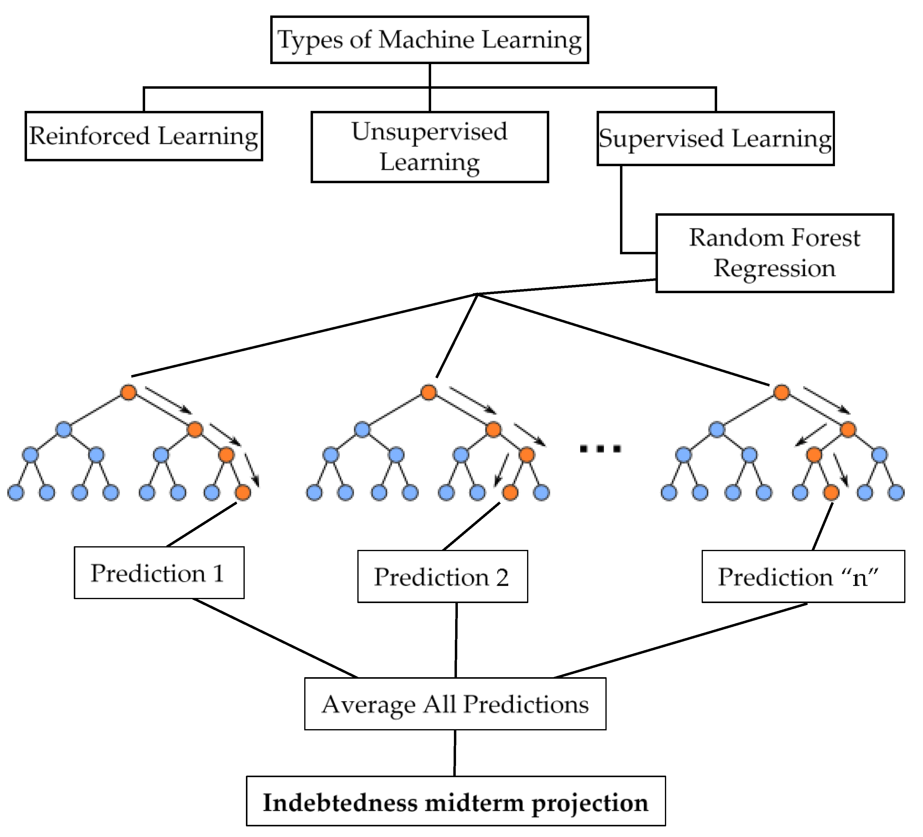
3.2. Description of Research Methodology

The random forest regression method is one of the most popular machine learning data models applied to data classification and regression analysis, and for predicting the future development of statistical series. Random forest regression is a supervised machine learning algorithm that combines multiple machine learning algorithms to produce more accurate models. Practically, random forest regression works by actually constructing a series of “trees” and averaging them. The methodology has its significant advantages over other algorithms. These include the following (Ao et al. 2019): greater flexibility in data learning, minimization of data errors, robustness of the algorithm, ability to efficiently process data with large numbers of predictors, eliminate deviations located below the average value of the predictions made, and feasibility in different aspects. At the same time, the model is not perfect, and its shortcomings are related to the fact that the process of developing “data forests” is slower than other algorithms; the initial data are presented in a large volume, which can make their final presentation difficult. The algorithm development process generally consists of creating a modelling sample, splitting the data into a modelling and validation sample, applying the algorithm to the sample, and final application of the model. Changes in the training samples lead to a significant change in the tree structure, as seen in the final results, which will be actually presented in this paper. The inputs that can be used to evaluate the model are the regression coefficients measuring the influence of the specified predictors, in combination with measures of the statistical significance and level of statistical error, such as mean absolute error (MAE), mean squared error (MSE), root mean squared error (RMSE), explained variance score, max error, median absolute error, and R2. Generally, MAE measures the sum of the absolute differences between the actual and predicted results, MSE measures the average of the squares of the errors, RMSE is the root-mean-square deviation of MSE, and explained variance score explains the dispersion of prediction errors and actual values (the higher the value of the indicator, the more adequate the model and the analysis performed) (Kharwal 2022). In addition to the explained variance score (EVS), for evaluating the state of the analytical value model, we also used the indicator for statistical expression of the relationship between the dependent and independent variables. In terms of value, the indicator used the principle of EVS.
The process of constructing of the approbated random forest regression is illustrated in Figure 1. The approbation of the random forest regression model demonstrated a high degree of accuracy and a low variance (Dudek 2022). With its high efficiency and flexibility of application, random forest regression is among the preferred machine learning algorithms. In a practical aspect, the application of the methodology could be useful in a number of fields. In particular, random forest regression has proven its effectiveness in various research areas, such as reward forecasting (Eichinger and Mayer 2022), evaluating the effects of macroprudential policy on real estate in Bulgaria (Prodanov et al. 2022b), estimating the fluid flow in curved pipes (Ganesh et al. 2021), water resources research (Tyralis et al. 2019), groundwater nitrate concentration modelling (Ouedraogo et al. 2019), and alternative forecasting in institutional research (He et al. 2018).
In this study, random forest regression is used to determine the factor impact on the indebtedness indicator, namely public debt-to-GDP in the EU member states, which will give us a clear idea of the financial measures and policies effected by the member states. In addition, country indicator forecasting is carried out in an attempt to identify countries with potentially growing public debt-to-GDP, which could have a negative impact on overall indebtedness in the established member state groups.

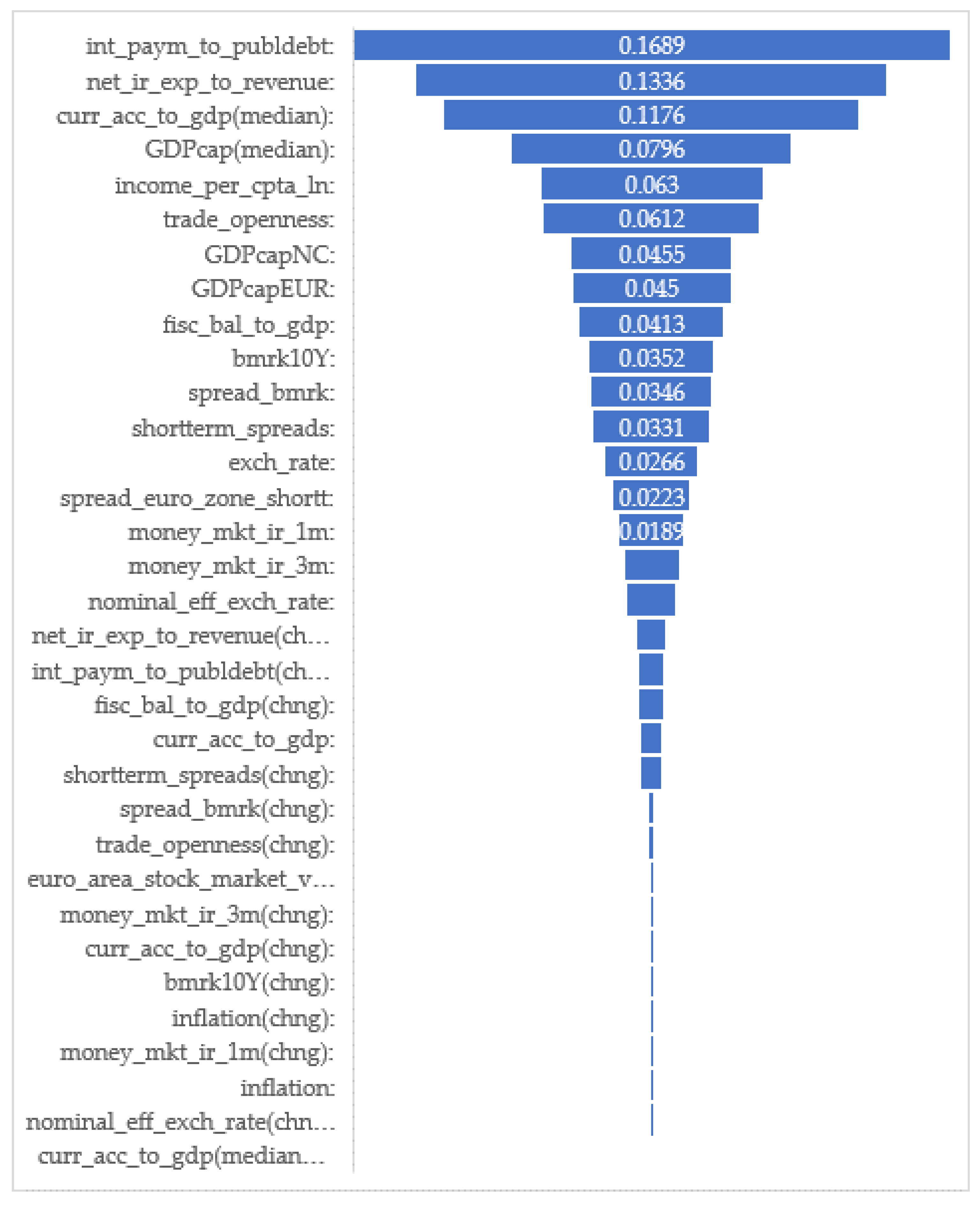
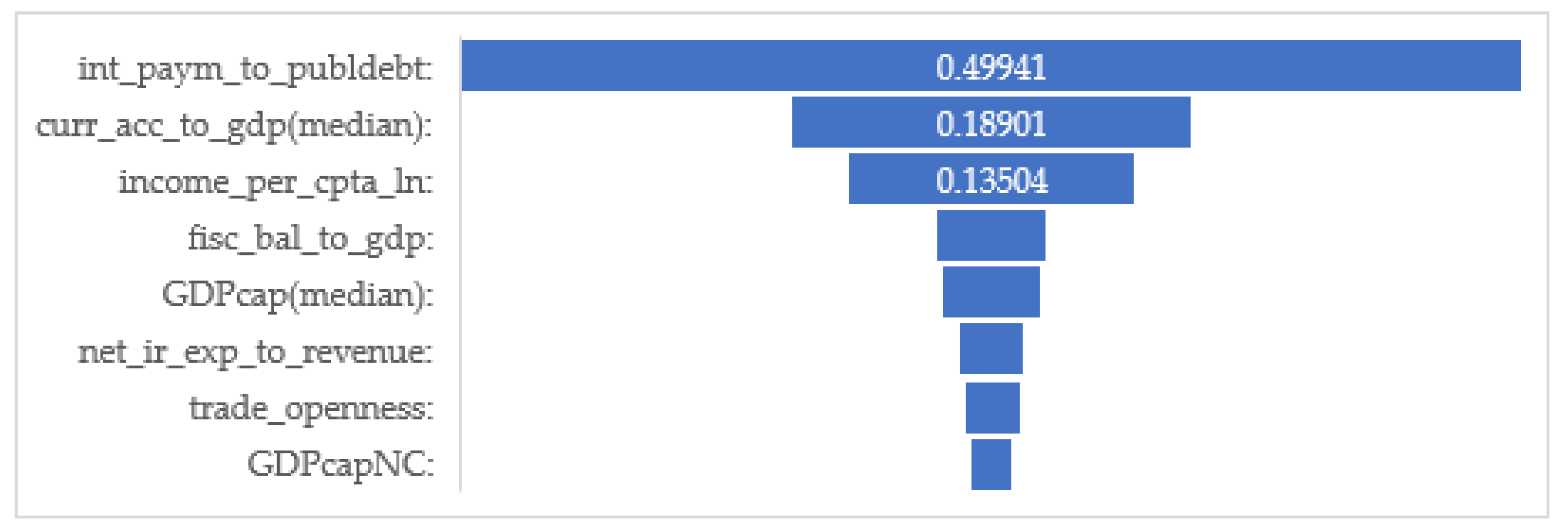
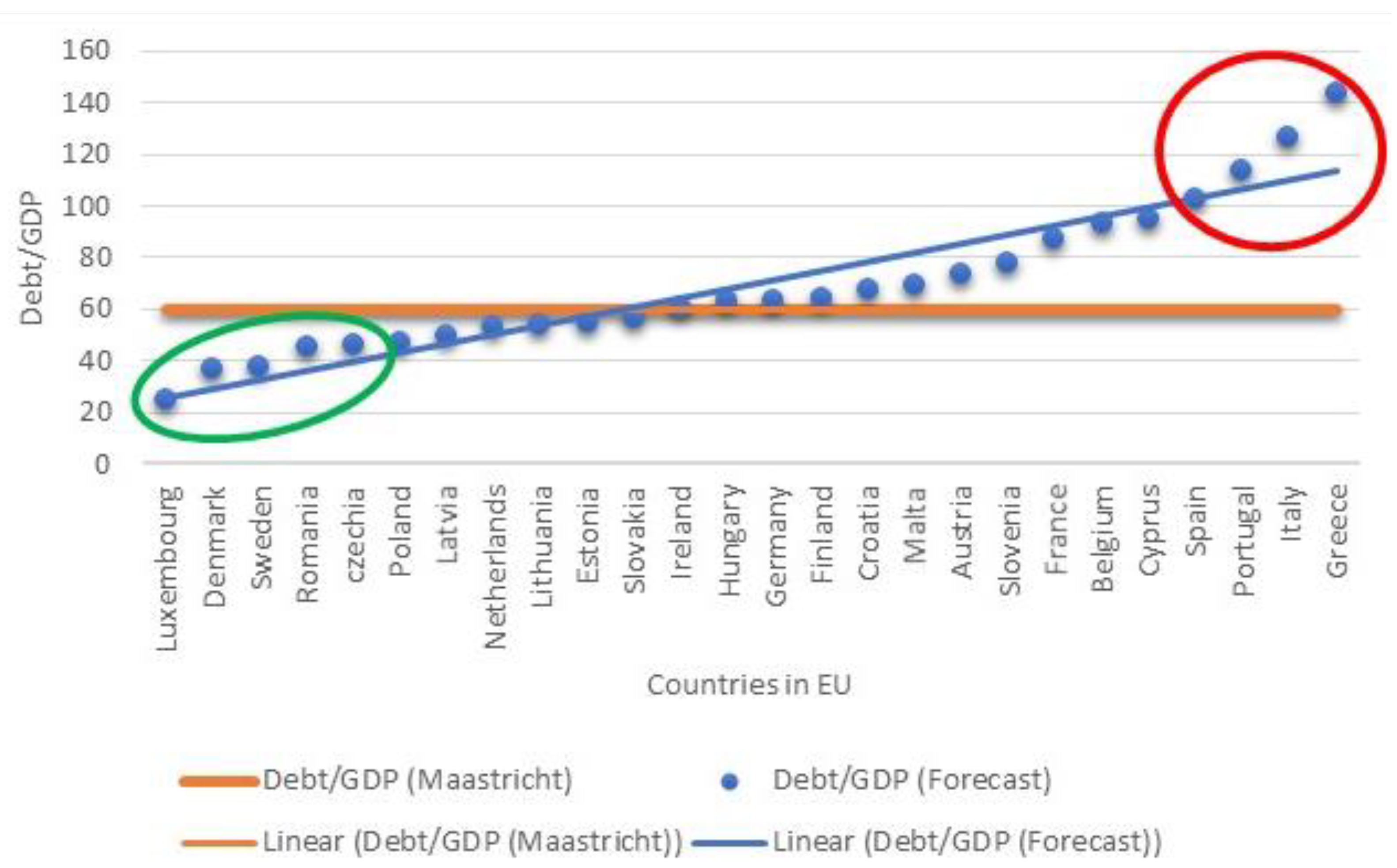
4. Empirical Results from Model Approbation

Being one of the essential and highly applicable additive machine learning models, random forest regression was used to determine the factor influence on sovereign indebtedness in terms of public debt-to-GDP ratio. The panel data were adapted for the purpose of the study and subjected to cross-validation of the data. For the purpose of parameter optimization, an additional test was performed on the validated sample. The process included two iterations with Version 1.0 of the model to assess the combined relationship of 33 indicators and with Version 2.0 to carry out a comparative test to determine the factor influence of the first eight significant indicators dominating the first iteration. The parameters of the two models can be defined as follows:
“#Final fit of random forest based on optimized params and cross validation on entire sample with 33 factors (ver. 1.0)
model = RandomForestRegressor (n_estimators = 782, min_samples_split = 2, min_samples_leaf = 1, max_features = ‘sqrt’, max_depth = 20, bootstrap = False, random_state = 1)
“#Final fit of random forest based on optimized params and cross validation on entire sample with most significant eight factors (ver. 2.0)
model = RandomForestRegressor (n_estimators = 68, min_samples_split = 5, min_samples_leaf = 2, max_features = ‘auto’, max_depth = 10, bootstrap = True, random_state = 1)
The model algorithms for optimization and cross validation performed in two iterations were used to trace the factor influence of the parameters in relation to the dependent variable (public debt-to-GDP) in the EU countries over the period January 2000 to December 2021, as shown in Figure 2 and Figure 3 below. In the first iteration, we used a wide range of independent variables with a direct or indirect influence on the dependent variable, while in the second iteration, we used only the eight most significant factors from the first iteration. The starting point for the initial selection of variables is the unanimously acknowledged theoretical relationships between the debt-to-GDP ratio and the influence of the analysed groups of factors. The indicators are ranked in descending order of their influence weight in Figure 2.
The indicators ranked in terms of their importance for changes in the public debt of EU member states are as follows: interest payments to public debt-to-GDP ratio (int_paym_to_publdebt) of 16.89%; net interest expense as a percentage of budget revenue (net_ir_exp_to_revenue) of 13.36%; the median value of the current account balance to GDP ratio (curr_acc_to_gdp(median)) of 11.76%; the median value of the Gross Domestic Product per capita (GDPcap(median)) of 7.96%; the income per capita (income_per_cpta_ln) of 6.3%, and trade openness (trade_openness) of 6.12%. The remaining factors are important as well, but have a significantly smaller degree of overall influence (less than 4%) on the dependent variable. The results show that according to the model, the most significant influence on the changes in the public debt-to-GDP are the focal and cointegration factors. Clearly, the dynamics of government interest expenditure emerge as a stronger predictor, relative to the raw monetary and market indicators.
To verify the model and its feasibility with different combinations of factors, a second iteration was performed using the eight most significant indicators (as the factor influence of the gross domestic product per capita in the national currency and in the Euro were identical, the ratio of the fiscal-balance-to-GDP was selected as the eighth factor). Because of the almost equal weight of GDPcapNC and GDPcapEUR (the difference being 0.0005 in the first iteration), in the second iteration of the test, we added the next most significant factor in terms of weight fisc_bal_to_gdp (0.0413). The results from the iteration with Version 2.0 of the model regarding the degree of factor influence are shown in Figure 3. Based on the second test of the described algorithm, a logical shift was observed in the degree of influence of the studied factors, while preserving the analytical value of the model.
The analysis of the available databases revealed a significant overall change in the status of the debt-to-GDP indicator. The largest negative changes (i.e., increases in the debt-to-GDP indicator) in retrospection were observed in Bulgaria, Estonia, Slovenia, and Romania. More significant decreases were observed in Ireland, the Netherlands, Denmark, Germany, and Malta. In this regard, the model foresees significant changes in the value of this indicator in the following EU member states: excessive increases in Bulgaria, Ireland, Malta, and Slovakia, and decreases in Spain, Belgium, Finland, Germany, Greece, and Italy.
According to the official statistics (up to 2021), iteration 2.0 of the model showed that the rate of changes in the newly created group of countries with a significant negative trend (i.e., Greece, Italy, Portugal, and France) varied between 13% and 16% on average for the period of 2023–2024. This is mainly due to the stabilization of the socio-economic situation of the countries after the significant impact of the COVID-19 pandemic (Zaharieva et al. 2022). However, the values of the debt-to-GDP indicator remained significantly above the assumed benchmark values for the EU. Should FPIG countries achieve a balance in the influencing debt factors and adopt harmonized fiscal policies, their high debt levels would not have a significant effect on the systematic risk of the EU as a whole.
According to the latest available Eurostat report (Euroindicators) of 23 January 2023 (Eurostat 2023) and the disclosed data regarding the government debt-to-GDP ratios, the top-ranking country (Estonia) is expected to lower its rank to the third position after Luxembourg and Sweden. Significant changes were found for the ranking of Bulgaria (from the second position in 2022 to eleventh position in the ranking of all EU member states) and Luxembourg, which assumed the leadership. According to the model, the changes at the bottom of the ranking (in the group of the most indebted countries of Greece, Italy, Portugal, and Spain) were also significant and imply that this group would comprise Greece, Italy, Portugal, and France.
Table 1 shows the statistics of the tested random forest regression models. They clearly show the statistical significance of both iterations (Versions 1.0 and Version 2.0) of the model. A high degree of correspondence was observed in the model performed based on the explained variance score—0.997546 (Ver. 1.0) and 0.992231 (Ver. 2.0). The significant values of the mean absolute error (MAE), mean squared error (MSE), root mean squared error (RMSE), and max error were explained by the variety of parameters used, which, for the purposes of the study, did not have a significant relationship. The mean explained variance calculated following the final parameter optimization based on cross-validation of the full model at “Mean expl_variance: %.3f (%.3f) (scores.mean(), scores.std())” shows that the model conforms to a degree approaching 100% for the purposes of achieving a solution to the originally stated research problem.
Considering the statistics of the two models presented above and the high degree of statistical significance obtained on the basis of algorithm and data optimization, a forecast of the debt-to-GDP indicator of the EU countries was made for the next two calendar years, which could be considered a period of economic and social recovery. Within this period, each country needs to implement accurate and analytically substantiated measures aimed to stabilize its fiscal indicators and its socio-economic position. Maintaining the level of the indicator within the required normative values is essential, both for the stability of the country itself and for the sustainability of the European Union in general. This is why, in order to determine which member states are likely to underperform in the coming years, a forecast of the public debt-to-GDP indicator for each individual EU member state was made (Appendix A). This gave us a clear idea of the expected trends for the sovereign debt and the member states that should take additional measures to limit the risk related to their government debt burden. In this regard, Figure 4 presents the average values of the forecasted public debt-to-GDP ratios for the period of 2023–2024, ver. 1.0 (33 indicators).
It is essential to note that due to the lack of data for some of the indicators for Bulgaria (they are not subject to national and international monitoring), the model could not be applied to our country. Despite the implemented optimizations in the algorithm, due to the risk of inaccuracy in the results obtained in version 1.0, the south-eastern border country of the EU was not included in the model, but was taken into account in the alternative version 2.0. The visualisation of the value of the convergence indicator for the next 24 months clearly distinguished two strategically important clusters—risk-independent (high-performing countries, marked with green circle in Figure 4), including Luxembourg, Denmark, Sweden, Romania, and the Czech Republic, and risky countries (which in their estimated values significantly exceed the maximum coefficient of 6o% and are positioned above the derived linear trend, marked with red circle in Figure 4), including Greece, Italy, Portugal, and Spain. The output of the estimated value was similar in version 2.0 (using the most significant 8 indicators from version 1.0), as shown in Figure 5. The results from this iteration show that the risk-independent group comprised Luxembourg, Sweden, Estonia, Denmark, and Romania (marked with green circle in Figure 5), while the group of countries at risk comprised Greece, Italy, Portugal, and France (marked with red circle in Figure 5). These results corresponded closely to a large body of previous research. They were of high significance in the context of the research of Baum et al. (2013), who investigated the impact of government debt on the per-capita growth rate of GDP. Their results suggest a non-linear effect with a turning point of 90–100%, beyond which the debt-to-GDP ratio had a negative impact on long-term growth.
Even more importantly, the study also reports that some of these effects started earlier at ratios of around 70 to 80%. As can be observed in Figure 5, the group of countries revealed as risky all corresponded to these two cases. This is especially worrying for France, as one of the EU and Euro area core countries, because the lower economic performance of France could hinder the entire EU GDP growth. There was another point of view to this problem in light of the abovementioned study of Globan and Matošec (2016). They concluded that in the quest for fiscal and financial stability it is more efficient to rely on greater GDP growth than less debt growth, i.e., it is more fruitful to “increase the denominator” rather than to “cut the numerator” of the debt-to-GDP ratio. From this point of view, evidently, when debt increases past a certain point, it is not only worsening the current and near future financial position of the country, but it is undermining in the long term the most efficient remedy against itself, which is GDP growth. This may put countries into a vicious circle, where more debt leads to less growth, which in turn leads to even more debt and can also create contagion effects (Kraft and Steffensen 2007) to other countries. In addition, according to a study by De Bruyckere et al. (2013), the debt-to-GDP ratio was one of the key country-specific drivers of the infamous bank-sovereign risk spillovers during the European debt crisis. Huyugüzel Kışla et al. (2022) also studied the spillovers during the European sovereign debt crisis and showed that a 1% increase in the debt-to-GDP ratio led to a 7 basis points increase in the CDS spread of one country and 2 basis points in the other countries with which the initial country is in close international trade relationships.

5. Conclusions

Public debt financing is a policy tool that solves current fiscal imbalances but creates medium-term (and often long-term) macroeconomic problems. The functioning of public systems in a pandemic environment undoubtedly necessitated measures that temporarily derogated the fiscal rules in the EU. In conditions of post-epidemic economic recovery, it has logically become relevant to derive forecasts for the medium-term indebtedness of the EU countries in conditions of several crises occurring simultaneously—shortage of energy resources, rising inflation levels, and the war in Ukraine. As a result of the analysis, in the medium term (2023–2024), a change in the composition of the four most indebted countries in the EU was identified, which transformed those in the worst four group. At the other end of the spectrum is the DRESL group of risk-independent countries, which includes Luxembourg, Sweden, Estonia, Denmark, and Romania. Which represents a new introduction to the EU debt topic with a positive character. It counterbalances the risky group of countries comprising Greece, Italy, Portugal, and France. The change in the composition of the group of countries with the worst indebtedness indicators led to negative effects, both for these countries and for the EU itself. The increase in the share of countries with the worst indebtedness indicators, according to the model’s forecast, is a factor that will increase systematic risk in the EU. The fact is that the derogation of fiscal restrictions as a measure to combat the consequences of the pandemic led to the accumulation of new debt. The fight against inflation objectively gives rise to increased interest rates, which are directly borne by all economic operators.
Deteriorated debt reputation at the level of systemic economies has turned from a studied problem into a typical feature of the EU. The medium-term forecast derived using the applied methodology shows changes in the indebtedness ranking for more than half of the member countries. At the same time, the discussion continues on the issue of whether and to what extent the Maastricht fiscal criteria are objective criteria for fiscal discipline. The political cycle in individual member states obviously provokes the process of the accumulation of public debts. Servicing these debts will create a dire need for reform and require governments to make unpopular austerity decisions. The outlined trend by the learning machines algorithm and specifically random forest regression show their wide field of application in deriving precise macroeconomic forecasts.

Author Contributions

Conceptualization, A.Z. and S.Z.; methodology, S.Z., D.K. and T.P.; software, S.Z. and T.P.; validation, S.Z., D.K. and T.P.; formal analysis, A.Z. and P.A.; investigation, A.Z., S.Z., D.K., P.A. and T.P.; resources, T.P.; data curation, T.P.; writing—original draft preparation, T.P., D.K. and S.Z.; writing—review and editing, A.Z. and P.A.; visualization, S.Z.; supervision, A.Z.; project administration, T.P.; funding acquisition, A.Z. All authors have read and agreed to the published version of the manuscript.

Funding

This research was funded by Academic Foundation “Professor Minko Rusenov, PhD” grant number 2023-01 and the Institute for Scientific Research of “D. A. Tsenov” Academy of Economics, Svishtov, Bulgaria.

Data Availability Statement

Upon request from the corresponding author.

Conflicts of Interest

The authors declare no conflict of interest.

Appendix A

Risks 11 00071 i001
Risks 11 00071 i002
Risks 11 00071 i003
Risks 11 00071 i004
Risks 11 00071 i005
Risks 11 00071 i006

References

  1. Albonico, Alice, and Patrizio Tirelli. 2020. Financial crises and sudden stops: Was the European monetary union crisis. Economic Modelling 93: 13–26. Available online: https://bit.ly/3msydMA (accessed on 8 September 2022). [CrossRef]
  2. Alexopoulou, Ioana, Irina Bunda, and Annalisa Ferrando. 2010. Determinants of government bond spreads in New EU countries. Eastern European Economics 48: 5–37. [Google Scholar] [CrossRef] [Green Version]
  3. Ao, Yile, Hongqi Li, Liping Zhu, Sikandar Ali, and Zhongguo Yang. 2019. The linear random forest algorithm and its advantages in machine learning assisted logging regression modeling. Journal of Petroleum Science and Engineering 174: 776–89. [Google Scholar] [CrossRef]
  4. Baum, Anja, Cristina Checherita-Westphal, and Philipp Rother. 2013. Debt and growth: New evidence for the euro area. Journal of International Money and Finance, 809–21. [Google Scholar] [CrossRef] [Green Version]
  5. Bezgin, Kostiantyn, Andrey Zahariev, Larysa Shaulska, Olha Doronina, Natela Tsiklashvili, and Natalia Wasilewska. 2022. Coevolution of education and business: Adaptive interaction. International Journal of Global Environmental Issues 21: 259–75. [Google Scholar] [CrossRef]
  6. Caner, Mehmet, Qingliang Fan, and Thomas Grennes. 2021. Partners in debt: An endogenous non-linear analysis of the effects of the effects of public and private debt on growth. International Review of Economics and Finance 76: 694–711. [Google Scholar] [CrossRef]
  7. De Bruyckere, Valerie, Maria Gerhardt, Glenn Schepens, and Rudi Vander Vennet. 2013. Bank/sovereign risk spillovers in the European debt crisis. Journal of Banking & Finance 37: 4793–809. [Google Scholar]
  8. Dudek, Grzegorz. 2022. A Comprehensive Study of Random Forest for Short-Term Load Forecasting. Energies 15: 7547. [Google Scholar] [CrossRef]
  9. Eichinger, Frank, and Moritz Mayer. 2022. Predicting Salaries with Random-Forest Regression. In Machine Learning and Data Analytics for Solving Business Problems, Methods, Applications, and Case Studies. Available online: https://www.researchgate.net/publication/366340005 (accessed on 5 January 2023).
  10. Em, Olga, Georgi Georgiev, Sergey Radukanov, and Mariana Petrova. 2022. Assessing the Market Risk on the Government Debt of Kazakhstan and Bulgaria in Conditions of Turbulence. Risks 10: 93. [Google Scholar] [CrossRef]
  11. Eurostat. 2023. Third Quarter of 2022 Government Debt down to 93.0% of GDP in Euro Area Down to 85.1% of GDP in EU. January 23. Available online: https://ec.europa.eu/eurostat/documents/2995521/15725185/2-23012023-AP-EN.pdf/ (accessed on 24 January 2023).
  12. Ganesh, Narayanan, Paras Jain, Amitava Choudhury, Prasun Dutta, Kanak Kalita, and Paolo Barsocchi. 2021. Random Forest Regression-Based Machine Learning Model for Accurate Estimation of Fluid Flow in Curved Pipes. Processes 9: 2095. [Google Scholar] [CrossRef]
  13. Geldiev, Ertan Mustafa, Nayden Valkov Nenkov, and Mariana Mateeva Petrova. 2018. Exercise of Machine Learning Using Some Python Tools and Techniques. Paper presented at CBU International Conference Proceedings 2018: Innovations in Science and Education, Prague, Czech Republic, March 21–23; pp. 1062–70. [Google Scholar] [CrossRef]
  14. Globan, Tomislav, and Marina Matošec. 2016. Public debt-to-GDP ratio in new EU member states: Cut the numerator or increase the denominator. Romanian Journal of Economic Forecasting 19: 57–72. [Google Scholar]
  15. Hauptmeier, Sebastian, and Christophe Kamps. 2022. Debt policies in the aftermath of COVID-19—The SGP’s debt. European Journal of Political Economy 75: 102187. [Google Scholar] [CrossRef] [PubMed]
  16. He, Lingjun, Richard A. Levine, Juanjuan Fan, Joshua Beemer, and Jeanne Stronach. 2018. Random Forest as a Predictive Analytics Alternative to Regression in Institutional Research. Practical Assessment, Research & Evaluation 23: 1. [Google Scholar] [CrossRef]
  17. Heppke-Falk, Kirsten, and Felix P. Hüfner. 2004. Expected Budget Deficits and Interest Rate Swap Spreads-Evidence for France, Germany and Italy. Frankfurt: Deutsche Bundesbank. [Google Scholar]
  18. Huyugüzel Kışla, Gül, Y. Gülnur Muradoğlu, and A. Özlem Önder. 2022. Spillovers from one country’s sovereign debt to CDS (credit default swap) spreads of others during the European crisis: A spatial approach. Journal of Asset Management 23: 277–96. [Google Scholar] [CrossRef]
  19. Insee. 2021. Convergence Criteria (Maastricht Treaty). January 28. Available online: http://bit.ly/3ZHMOSz (accessed on 15 September 2022).
  20. Kharwal, Aman. 2022. Explained Variance in Machine Learning. Available online: https://thecleverprogrammer.com/2021/06/25/explained-variance-in-machine-learning/ (accessed on 25 June 2021).
  21. Kraft, Holger, and Mogens Steffensen. 2007. Bankruptcy, counterparty risk, and contagion. Review of Finance 11: 209–52. [Google Scholar] [CrossRef]
  22. Laktionova, Oleksandra, Oleksandr Dobrovolskyi, Tatyana Sergeevna Karpova, and Andrey Zahariev. 2019. Cost Efficiency of Applying Trade Finance for Agricultural Supply Chains. Management Theory and Studies for Rural Business and Infrastructure Development 41: 62–73. [Google Scholar] [CrossRef]
  23. Mackiewicz-Łyziak, Joanna, and Tomasz Łyziak. 2019. A new test for fiscal sustainability with endogenous sovereign bond yields: Evidence for EU economies. Economic Modelling 82: 136–51. [Google Scholar] [CrossRef]
  24. Maltritz, Dominik, and Sebastian Wüste. 2014. Determinants of budget deficits in Europe: The role and relations of fiscal. Economic Modelling 48: 222–36. [Google Scholar] [CrossRef]
  25. Ostrihon, Filip. 2020. Exploring macroeconomic imbalances through EU Alert. European Journal of Political Economy 75: 102188. [Google Scholar] [CrossRef]
  26. Ouedraogo, Issoufou, Pierre Defourny, and Marnik Vanclooster. 2019. Application of random forest regression and comparison of its performance to multiple linear regression in modeling groundwater nitrate concentration at the African continent scale. Hydrogeology Journal 27: 1081–98. [Google Scholar] [CrossRef]
  27. Posta, Pompeo Della. 2021. Government size and speculative attacks on public debt. International Review of Economics and Finance 72: 79–89. [Google Scholar] [CrossRef]
  28. Prodanov, Stoyan, and Lyudmil Naydenov. 2020. Theoretical, qualitative and quantitative aspects of municipal fiscal autonomy in Bulgaria. Ikonomicheski Izsledvania 29: 126–50. Available online: https://bit.ly/3rmXlTL (accessed on 10 June 2021).
  29. Prodanov, Stoyan, Orlin Yaprakov, and Silvia Zarkova. 2022a. CAMEL evaluation of the banks in Bulgaria. Economic Alternatives 2022: 201–19. [Google Scholar] [CrossRef]
  30. Prodanov, Stoyan, Petko Angelov, and Silvia Zarkova. 2022b. Real Estate in Bulgaria from the global financial crisi to the COVID-19 crisis-effects of macroprudential policy: Evidence from Bulgaria. Paper presented at 87th International Scientific Conference on Economic and Social Development—“Economics, Management, Finance and Banking”, Svishtov, Bulgaria, September 28–30; pp. 162–70. [Google Scholar]
  31. Roleders, Viktoriia, Tetyana Oriekhova, and Galina Zaharieva. 2022. Circular Economy as a Model of Achieving Sustainable Development. Problemy Ekorozwoju—Problems of Sustainable Development 17: 178–85. [Google Scholar] [CrossRef]
  32. Sakuragawaa, Masaya, and Yukie Sakuragawa. 2020. Government fiscal projection and debt sustainability. Japan & The World Economy 54: 101010. [Google Scholar] [CrossRef]
  33. TIBCO. 2023. What Is a Random Forest? Available online: https://www.tibco.com/reference-center/what-is-a-random-forest (accessed on 10 December 2022).
  34. Tyralis, Hristos, Georgia Papacharalampous, and Andreas Langousis. 2019. A Brief Review of Random Forests for Water Scientists and Practitioners and Their Recent History in Water Resources. Water 11: 910. [Google Scholar] [CrossRef] [Green Version]
  35. Zahariev, Andrey, Anelia Radulova, Aleksandrina Aleksandrova, and Mariana Petrova. 2021. Fiscal sustainability and fiscal risk in the EU: Forecasts and challenges in terms of COVID-19. Entrepreneurship and Sustainability Issues 8: 618–32. [Google Scholar] [CrossRef] [PubMed]
  36. Zahariev, Andrey, Mikhail Zveryakov, Stoyan Prodanov, Galina Zaharieva, Petko Angelov, Silvia Zarkova, and Mariana Petrova. 2020. Debt management evaluation through support vector machines: On the example of Italy and Greece. Entrepreneurship and Sustainability Issues 7: 2382–93. [Google Scholar] [CrossRef] [Green Version]
  37. Zahariev, Andrey, Petko Angelov, and Silvia Zarkova. 2022. Estimation of Bank Profitability Using Vector Error Correction Model and Support Vector Regression. Economic Alternatives 2022: 157–70. [Google Scholar] [CrossRef]
  38. Zaharieva, Galina, Onnik Tarakchiyan, and Andrey Zahariev. 2022. Market capitalization factors of the Bulgarian pharmaceutical sector in pandemic environment. Business Management XXXII: 35–51. Available online: https://www.scopus.com/record/display.uri?eid=2-s2.0-85144992057&origin=resultslist (accessed on 10 January 2023).
Figure 1. Structuring the Random Forest Regression. Source: upgraded author’s model based on initial findings of (TIBCO 2023).
Risks 11 00071 g001
Figure 2. Random Forest Regression ver. 2.0—Parametric assessment of the factor influence of all indicators on the government debt-to-GDP ratio. Source: Authors’ calculations.
Risks 11 00071 g002
Figure 3. Random Forest Regression ver. 2.0—Parametric assessment of the factor influence of selected indicators on the government debt-to-GDP ratio. Source: authors’ calculations.
Risks 11 00071 g003
Figure 4. Average values of the forecast debt-to-GDP ratio for the period 2023–2024, Ver. 1.0 (33 indicators). Source: authors’ calculations.
Risks 11 00071 g004
Figure 5. Average values of the forecast debt-to-GDP ratio for the period 2023–2024, Ver. 2.0 (8 indicators). Source: authors’ calculations.
Risks 11 00071 g005
Table 1. Model statistics. Source: authors’ calculations.
StatisticsValues
Ver. 1.0 (33 Indicators)Ver. 2.0 (8 Indicators)
Mean Absolute Error (MAE):0.9737151.820823
Mean Squared Error (MSE):3.13863410.294671
Root Mean Squared Error (RMSE):1.7716193.208531
Explained Variance Score:0.9975460.992231
Max Error:28.1081827.173953
Median Absolute Error:0.5639781.026739
R2:0.997545 **0.992228 *
Mean explained variance:0.998 (0.000) **0.993 (0.000) *
Note: 10%, and 5%, significance levels are represented by the symbols *, **, respectively.
Disclaimer/Publisher’s Note: The statements, opinions and data contained in all publications are solely those of the individual author(s) and contributor(s) and not of MDPI and/or the editor(s). MDPI and/or the editor(s) disclaim responsibility for any injury to people or property resulting from any ideas, methods, instructions or products referred to in the content.

