Appendix A
Table A1.
Descriptive statistics: mean and standard deviation (SD) for 20,784 policyholders in seven observed months in 2018 and 2019.
Table A1.
Descriptive statistics: mean and standard deviation (SD) for 20,784 policyholders in seven observed months in 2018 and 2019.
| Mean | Month 6 | Month 7 | Month 8 | Month 9 | Month 10 | Month 11 | Month 12 | Total |
|---|
| Telematics variables | | | | | | | | |
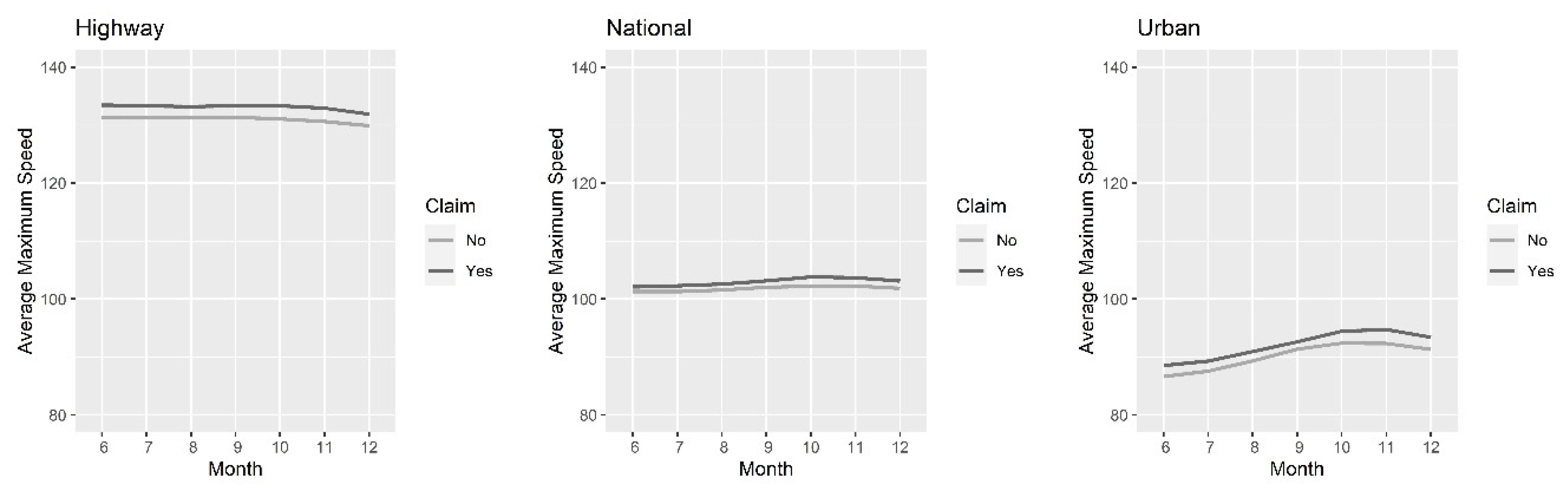
| Tele_km_total_urban | 361.745 | 353.987 | 345.384 | 331.785 | 322.242 | 303.230 | 283.157 | 328.790 |
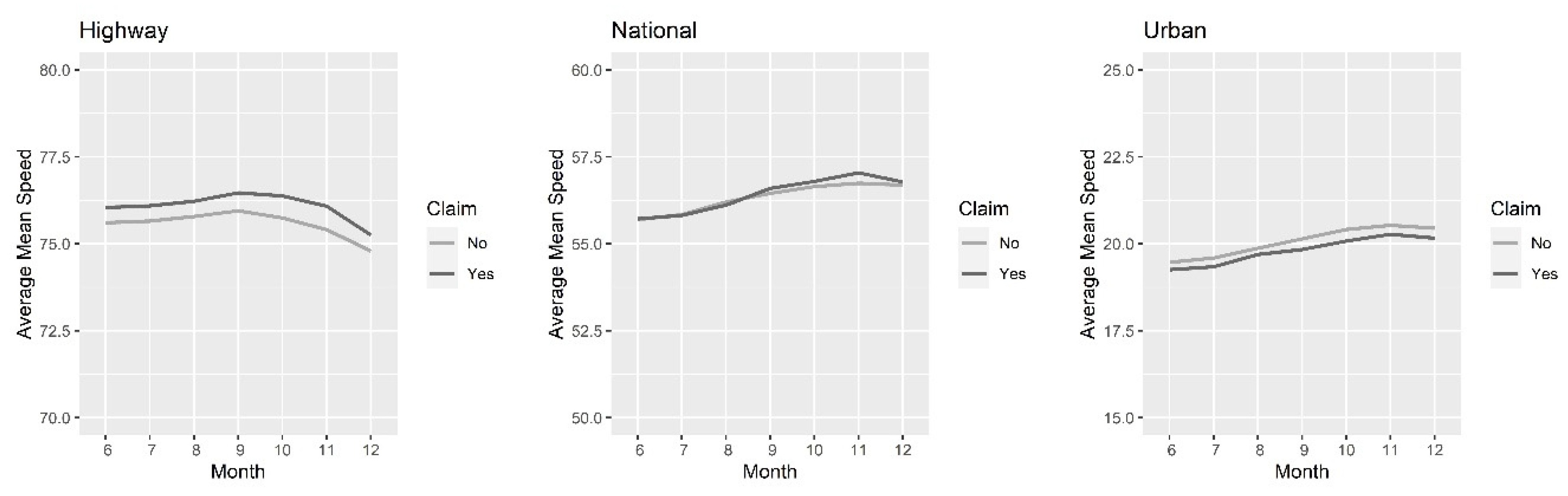
| Tele_speed_mean_urban | 19.422 | 19.540 | 19.833 | 20.077 | 20.340 | 20.476 | 20.384 | 20.010 |
| Tele_speed_max_highway | 131.781 | 131.704 | 131.712 | 131.793 | 131.557 | 131.121 | 130.341 | 131.430 |
| Weather conditions | | | | | | | | |
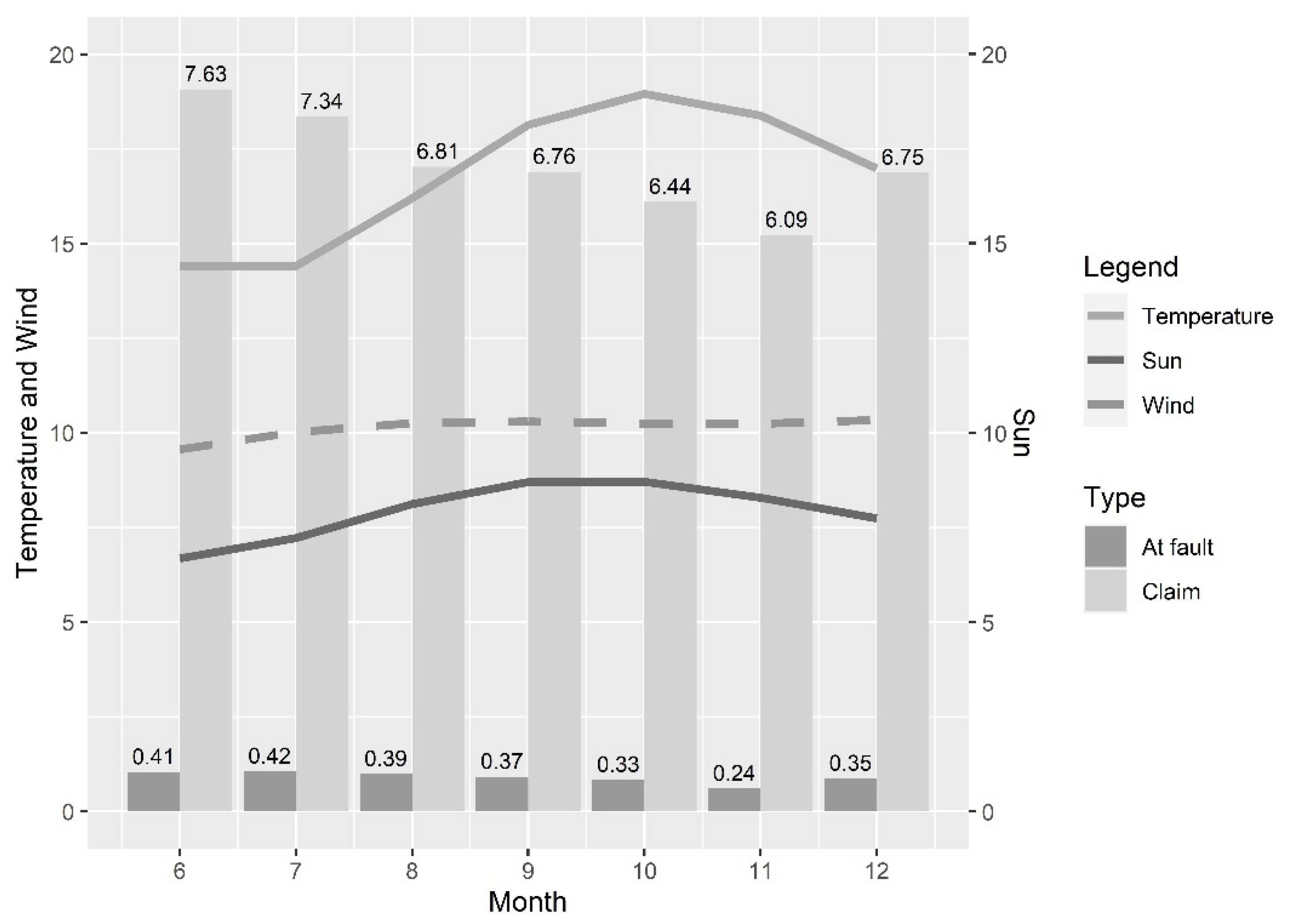
| Wind | 9.560 | 10.021 | 10.259 | 10.297 | 10.251 | 10.246 | 10.343 | 10.140 |
| Temperature | 14.404 | 14.407 | 16.202 | 18.138 | 18.959 | 18.386 | 16.986 | 16.783 |
| Sun | 6.682 | 7.219 | 8.118 | 8.702 | 8.706 | 8.289 | 7.740 | 7.922 |
| Responses | | | | | | | | |
| Claims | 0.076 | 0.073 | 0.068 | 0.068 | 0.064 | 0.061 | 0.068 | 0.068 |
| At-fault third-party liability | 0.004 | 0.004 | 0.004 | 0.004 | 0.003 | 0.002 | 0.003 | 0.004 |
| S.D. | Month 6 | Month 7 | Month 8 | Month 9 | Month 10 | Month 11 | Month 12 | Total |
| Telematics variables | | | | | | | | |
| Tele_km_total_urban | 310.455 | 297.183 | 293.006 | 275.432 | 265.530 | 245.056 | 230.455 | 230.455 |
| Tele_speed_mean_urban | 5.524 | 5.598 | 5.715 | 5.764 | 5.928 | 6.056 | 6.075 | 6.075 |
| Tele_speed_max_highway | 15.583 | 15.527 | 15.618 | 16.002 | 16.131 | 16.737 | 16.934 | 16.934 |
| Weather conditions | | | | | | | | |
| Wind | 1.802 | 1.877 | 1.734 | 1.666 | 1.657 | 1.739 | 1.864 | 1.864 |
| Temperature | 4.936 | 5.311 | 5.827 | 5.894 | 5.864 | 6.024 | 6.080 | 6.080 |
| Sun | 2.078 | 2.348 | 2.432 | 2.337 | 2.319 | 2.372 | 2.364 | 2.364 |
| Responses | | | | | | | | |
| Claims | 0.491 | 0.481 | 0.467 | 0.466 | 0.440 | 0.407 | 0.443 | 0.443 |
| At-fault third-party liability | 0.064 | 0.065 | 0.063 | 0.061 | 0.058 | 0.049 | 0.059 | 0.059 |
Table A2.
Cross-table with the parameter estimates of random effects and fixed-effects Poisson panel data models, with p-values, for the total number of claims (left) and at-fault third-party liability (TPL) claims (right) per month and per insured based on the seven observed months in 2018 and 2019. The models consider the average number of sunshine hours per day as explanatory variable describing weather conditions.
| Variable | All Claims | Only At-Fault TPL Claims |
|---|
| Random Effects | Fixed Effects | Random Effects | Fixed Effects |
|---|
| Parameter | p-Value | Parameter | p-Value | Parameter | p-Value | Parameter | p-Value |
|---|
| Intercept | −2.688 | <0.001 | - | - | −6.049 | <0.001 | - | - |
| lag(claims *) | −0.445 | <0.001 | −0.569 | <0.001 | −1.177 | 0.261 | −4.357 | <0.001 |
| Sun | 0.001 | 0.979 | 0.004 | 0.438 | −0.025 | 0.209 | −0.003 | 0.887 |
| Tele_km_total_urban ** | 0.116 | 0.018 | −0.223 | <0.001 | 0.789 | <0.001 | 0.015 | 0.951 |
| Tele_speed_mean_urban | −0.020 | <0.001 | −0.020 | <0.001 | −0.022 | 0.014 | −0.028 | 0.043 |
| Tele_speed_max_highway | 0.003 | <0.001 | −0.001 | 0.328 | 0.006 | 0.048 | −0.011 | 0.045 |
| στ | 0.158 | <0.001 | - | - | 1.000 | 0.159 | - | - |
| AIC | 58,920.18 | 26,836.56 | 5787.84 | 1426.87 |
Table A3.
Cross-table with the parameter estimates of random effects and fixed-effects Poisson panel data models, with p-values, for the total number of claims (left) and at-fault third-party liability (TPL) claims (right) per month and per insured based on the seven observed months in 2018 and 2019. The models consider the average monthly temperature as explanatory variable describing weather conditions.
| Variable | All Claims | Only At-Fault TPL Claims |
|---|
| Random Effects | Fixed Effects | Random Effects | Fixed Effects |
|---|
| Parameter | p-Value | Parameter | p-Value | Parameter | p-Value | Parameter | p-Value |
|---|
| Intercept | −2.680 | <0.001 | - | - | −6.022 | <0.001 | - | - |
| lag(claims *) | −0.444 | <0.001 | −0.570 | <0.001 | −1.177 | 0.261 | −4.357 | <0.001 |
| Temperature | −0.001 | 0.788 | 0.002 | 0.331 | −0.013 | 0.116 | −0.002 | 0.857 |
| Tele_km_total_urban ** | 0.116 | 0.017 | −0.224 | <0.001 | 0.797 | <0.001 | 0.016 | 0.946 |
| Tele_speed_mean_urban | −0.020 | <0.001 | −0.020 | <0.001 | −0.021 | 0.016 | −0.028 | 0.043 |
| Tele_speed_max_highway | 0.003 | <0.001 | −0.001 | 0.317 | 0.005 | 0.056 | −0.011 | 0.046 |
| στ | 0.158 | <0.001 | - | - | 1.004 | 0.160 | - | - |
| AIC | 58,920.11 | 26,836.22 | 5786.94 | 1426.86 |
Table A4.
Cross-table with the parameter estimates of random effects and fixed-effects Poisson panel data models, with p-values. for the total number of claims (left) and at-fault third party liability (TPL) claims (right) per month and per insured based on the seven observed months in 2018 and 2019. Monthly maximum daily average wind speed is introduced as the weather-related regressor.
| Variable | ALL Claims | Only at Fault TPL Claims |
|---|
| Random Effects | Fixed Effects | Random Effects | Fixed Effects |
|---|
| Parameter | p-Value | Parameter | p-Value | Parameter | p-Value | Parameter | p-Value |
|---|
| Intercept | −2.839 | <0.001 | - | - | −6.920 | <0.001 | - | - |
| lag(claims *) | −0.444 | <0.001 | −0.569 | <0.001 | −1.187 | 0.257 | −4.358 | <0.001 |
| Wind max | 0.011 | 0.038 | 0.006 | 0.279 | 0.053 | 0.010 | 0.036 | 0.165 |
| Tele_km_total_urban ** | 0.120 | 0.014 | −0.218 | <0.001 | 0.788 | <0.001 | 0.039 | 0.870 |
| Tele_speed_mean_urban | −0.020 | <0.001 | −0.020 | <0.001 | −0.023 | 0.009 | −0.028 | 0.045 |
| Tele_speed_max_highway | 0.003 | <0.001 | −0.001 | 0.381 | 0.006 | 0.034 | −0.011 | 0.043 |
| στ | 0.158 | <0.001 | - | - | 1.008 | 0.161 | - | - |
| AIC | 58,915.90 | 26,836.00 | 5782.95 | 1424.98 |
Table A5.
Cross-table with the parameter estimates of random effects and fixed-effects Poisson panel data models, with p-values, for the total number of claims (left) and at-fault third party liability (TPL) claims (right) per month and per insured based on the seven observed months in 2018 and 2019. The models consider the monthly maximum daily average of sunshine hours as explanatory variable describing weather conditions.
| Variable | All Claims | Only At Fault TPL Claims |
|---|
| Random Effects | Fixed Effects | Random Effects | Fixed Effects |
|---|
| Parameter | p-Value | Parameter | p-Value | Parameter | p-Value | Parameter | p-Value |
|---|
| Intercept | −2.723 | <0.001 | - | - | −6.032 | <0.001 | - | - |
| lag(claims *) | −0.445 | <0.001 | −0.570 | <0.001 | −1.177 | 0.261 | −4.360 | <0.001 |
| Sun max | 0.005 | 0.391 | 0.009 | 0.088 | −0.022 | 0.284 | 0.009 | 0.724 |
| Tele_km_total_urban ** | 0.115 | 0.019 | −0.223 | <0.001 | 0.788 | <0.001 | 0.017 | 0.943 |
| Tele_speed_mean_urban | −0.020 | <0.001 | −0.020 | <0.001 | −0.022 | 0.014 | −0.029 | 0.037 |
| Tele_speed_max_highway | 0.003 | 0.001 | −0.001 | 0.295 | 0.006 | 0.047 | −0.011 | 0.040 |
| στ | 0.158 | <0.001 | - | - | 1.001 | 0.160 | - | - |
| AIC | 58,919.45 | 26,834.25 | 5788.27 | 1426.77 |
Table A6.
Cross-table with the parameter estimates of random effects and fixed-effects Poisson panel data models, with p-values, for the total number of claims (left) and at-fault third party liability (TPL) claims (right) per month and per insured based on the seven observed months in 2018 and 2019. The models consider the monthly maximum daily average temperature as explanatory variable describing weather conditions.
| Variable | All Claims | Only at Fault TPL Claims |
|---|
| Random Effects | Fixed Effects | Random Effects | Fixed Effects |
|---|
| Parameter | p-Value | Parameter | p-Value | Parameter | p-Value | Parameter | p-Value |
|---|
| Intercept | −2.702 | <0.001 | - | - | −5.981 | <0.001 | - | - |
| lag(claims *) | −0.445 | <0.001 | −0.570 | <0.001 | −1.176 | 0.261 | −4.357 | <0.001 |
| Temperature max | 0.001 | 0.581 | 0.004 | 0.053 | −0.014 | 0.084 | −0.001 | 0.881 |
| Tele_km_total_urban ** | 0.114 | 0.020 | −0.229 | <0.001 | 0.805 | <0.001 | 0.017 | 0.942 |
| Tele_speed_mean_urban | −0.020 | <0.001 | −0.020 | <0.001 | −0.021 | 0.016 | −0.028 | 0.042 |
| Tele_speed_max_highway | 0.003 | <0.001 | −0.001 | 0.273 | 0.006 | 0.053 | −0.011 | 0.046 |
| στ | 0.158 | <0.001 | - | - | 1.007 | 0.161 | - | - |
| AIC | 58,919.88 | 26,833.42 | 5786.42 | 1426.87 |
Table A7.
Cross-table with the parameter estimates of random effects and fixed-effects Poisson panel data models, with p-values. for the total number of claims (left) and at-fault third party liability (TPL) claims (right) per month and per insured based on the eight observed months in 2018 and 2019, i.e., month 5 is included.
| Variable | All Claims | Only at Fault TPL Claims |
|---|
| Random Effects | Fixed Effects | Random Effects | Fixed Effects |
|---|
| Parameter | p-Value | Parameter | p-Value | Parameter | p-Value | Parameter | p-Value |
|---|
| Intercept | −3.049 | <0.001 | - | - | −7.309 | <0.001 | - | - |
| lag(claims *) | −0.421 | <0.001 | −0.535 | <0.001 | −1.373 | 0.184 | −4.389 | <0.001 |
| Wind | 0.019 | 0.006 | 0.014 | 0.055 | 0.077 | 0.002 | 0.063 | 0.054 |
| Tele_km_total_urban ** | 0.064 | 0.145 | −0.275 | <0.001 | 0.727 | <0.001 | −0.042 | 0.842 |
| Tele_speed_mean_urban | 0.016 | <0.001 | −0.016 | <0.001 | −0.018 | 0.024 | −0.018 | 0.148 |
| Tele_speed_max_highway | 0.004 | <0.001 | <0.001 | 0.911 | 0.008 | 0.004 | −0.007 | 0.145 |
| στ | 0.183 | <0.001 | - | - | 1.151 | 0.125 | - | - |
| AIC | 70,710.83 | 34,887.78 | 6893.57 | 1886.79 |
Table A8.
Cross-table with the parameter estimates of random effects and fixed-effects Poisson panel data models, with p-values, for the total number of claims (left) and at-fault third party liability (TPL) claims (right) per month and per insured based on the eight observed months in 2018 and 2019, i.e., month 5 is included. The models consider the average number of sunshine hours per day as explanatory variable describing weather conditions.
| Variable | All Claims | Only at Fault TPL Claims |
|---|
| Random Effects | Fixed Effects | Random Effects | Fixed Effects |
|---|
| Parameter | p-Value | Parameter | p-Value | Parameter | p-Value | Parameter | p-Value |
|---|
| Intercept | −2.842 | <0.001 | - | - | −6.356 | <0.001 | - | - |
| lag(claims *) | −0.420 | <0.001 | −0.534 | <0.001 | −1.354 | 0.190 | −4.375 | <0.001 |
| Sun | 0.001 | 0.834 | 0.004 | 0.425 | −0.013 | 0.462 | 0.001 | 0.944 |
| Tele_km_total_urban ** | 0.059 | 0.177 | −0.283 | <0.001 | 0.731 | <0.001 | −0.081 | 0.701 |
| Tele_speed_mean_urban | −0.016 | <0.001 | −0.016 | <0.001 | −0.016 | 0.050 | −0.018 | 0.149 |
| Tele_speed_max_highway | 0.004 | <0.001 | >−0.001 | 0.965 | 0.007 | 0.011 | −0.007 | 0.120 |
| στ | 0.183 | <0.001 | - | - | 1.139 | 0.123 | - | - |
| AIC | 70,718.47 | 34,890.80 | 6902.71 | 1890.49 |
Table A9.
Cross-table with the parameter estimates of random effects and fixed-effects Poisson panel data models, with p-values, for the total number of claims (left) and at-fault third party liability (TPL) claims (right) per month and per insured based on the eight observed months in 2018 and 2019, i.e., month 5 is included. The models consider the average monthly temperature as explanatory variable describing weather conditions.
| Variable | All Claims | Only at Fault TPL Claims |
|---|
| Random Effects | Fixed Effects | Random Effects | Fixed Effects |
|---|
| Parameter | p-Value | Parameter | p-Value | Parameter | p-Value | Parameter | p-Value |
|---|
| Intercept | −2.817 | <0.001 | - | - | −6.283 | <0.001 | - | - |
| lag(claims *) | −0.420 | <0.001 | −0.534 | <0.001 | −1.355 | 0.190 | −4.373 | <0.001 |
| Temperature | −0.002 | 0.377 | <0.001 | 0.982 | −0.010 | 0.163 | −0.005 | 0.545 |
| Tele_km_total_urban ** | 0.061 | 0.168 | −0.284 | <0.001 | 0.738 | <0.001 | −0.081 | 0.698 |
| Tele_speed_mean_urban | −0.016 | <0.001 | −0.016 | <0.001 | −0.015 | 0.054 | −0.017 | 0.170 |
| Tele_speed_max_highway | 0.004 | <0.001 | >−0.001 | 0.987 | 0.007 | 0.012 | −0.007 | 0.136 |
| στ | 0.183 | <0.001 | - | - | 1.141 | 0.123 | - | - |
| AIC | 70,717.74 | 34,891.44 | 6901.30 | 1890.13 |
Table A10.
Cross-table with the parameter estimates of random effects and fixed-effects Poisson panel data models, with p-values. for the total number of claims (left) and at-fault third party liability (TPL) claims (right) per month and per insured based on the seven observed months in 2018 and 2019. Interactions are included.
| Variable | All Claims | Only At Fault TPL Claims |
|---|
| Random Effects | Fixed Effects | Random Effects | Fixed Effects |
|---|
| Parameter | p-Value | Parameter | p-Value | Parameter | p-Value | Parameter | p-Value |
|---|
| Intercept | −3.342 | <0.001 | - | - | −6.197 | 0.009 | - | - |
| lag(claims *) | −0.445 | <0.001 | −0.569 | <0.001 | −1.203 | 0.251 | −4.370 | <0.001 |
| Wind | 0.061 | 0.295 | 0.015 | 0.809 | −0.011 | 0.961 | −0.042 | 0.872 |
| Tele_km_total_urban ** | 0.083 | 0.752 | −0.335 | 0.244 | 0.847 | 0.253 | −0.983 | 0.375 |
| Tele_speed_mean_urban | −0.007 | 0.609 | <0.001 | 0.977 | −0.067 | 0.183 | −0.061 | 0.295 |
| Tele_speed_max_highway | 0.005 | 0.295 | −0.004 | 0.419 | 0.005 | 0.762 | −0.012 | 0.551 |
| Wind*Tele_km_total_urban ** | 0.004 | 0.883 | 0.011 | 0.678 | −0.005 | 0.941 | 0.103 | 0.324 |
| Wind*Tele_speed_mean_urban | −0.001 | 0.291 | −0.002 | 0.143 | 0.004 | 0.388 | 0.003 | 0.563 |
| Wind*Tele_speed_max_highway | >−0.001 | 0.799 | <0.001 | 0.538 | <0.001 | 0.922 | <0.001 | 0.931 |
| στ | 0.158 | <0.001 | - | - | 1.006 | 0.161 | - | - |
| AIC | 58,916.38 | 26,837.19 | 5784.357 | 1426.86 |
Table A11.
Cross-table with the parameter estimates of random effects and fixed-effects Poisson panel data models, with p-values, for the total number of claims (left) and at-fault third party liability (TPL) claims (right) per month and per insured based on the seven observed months in 2018 and 2019. The models consider the average number of sunshine hours per day as explanatory variable describing weather conditions. Interactions are included.
| Variable | All Claims | Only at Fault TPL Claims |
|---|
| Random Effects | Fixed Effects | Random Effects | Fixed Effects |
|---|
| Parameter | p-Value | Parameter | p-Value | Parameter | p-Value | Parameter | p-Value |
|---|
| Intercept | −3.655 | <0.001 | - | - | −7.481 | <0.001 | - | - |
| lag(claims *) | −0.445 | <0.001 | −0.569 | <0.001 | −1.207 | 0.250 | −4.366 | <0.001 |
| Sun | 0.120 | 0.004 | 0.141 | 0.001 | 0.156 | 0.350 | 0.377 | 0.047 |
| Tele_km_total_urban ** | −0.366 | 0.012 | −0.717 | <0.001 | 0.336 | 0.468 | −0.759 | 0.239 |
| Tele_speed_mean_urban | −0.002 | 0.807 | 0.002 | 0.833 | 0.005 | 0.872 | 0.030 | 0.397 |
| Tele_speed_max_highway | 0.009 | <0.001 | 0.005 | 0.059 | 0.014 | 0.157 | 0.005 | 0.644 |
| Sun*Tele_km_total_urban ** | 0.059 | <0.001 | 0.061 | 0.001 | 0.055 | 0.306 | 0.093 | 0.205 |
| Sun*Tele_speed_mean_urban | −0.002 | 0.012 | −0.003 | 0.005 | −0.003 | 0.350 | −0.007 | 0.083 |
| Sun*Tele_speed_max_highway | −0.001 | 0.013 | −0.001 | 0.009 | −0.001 | 0.389 | −0.002 | 0.123 |
| στ | 0.158 | <0.001 | - | - | 0.970 | 0.151 | - | - |
| AIC | 58,904.37 | 26,818.82 | 5791.49 | 1426.45 |
Table A12.
Cross-table with the parameter estimates of random effects and fixed-effects Poisson panel data models, with p-values, for the total number of claims (left) and at-fault third party liability (TPL) claims (right) per month and per insured based on the seven observed months in 2018 and 2019. The models consider the average monthly temperature as explanatory variable describing weather conditions. Interactions are included.
| Variable | All Claims | Only at Fault TPL Claims |
|---|
| Random Effects | Fixed Effects | Random Effects | Fixed Effects |
|---|
| Parameter | p-Value | Parameter | p-Value | Parameter | p-Value | Parameter | p-Value |
|---|
| Intercept | −2.952 | <0.001 | - | - | −6.480 | <0.001 | - | - |
| lag(claims *) | −0.445 | <0.001 | −0.570 | <0.001 | −1.190 | 0.256 | −4.367 | <0.001 |
| Temperature | 0.015 | 0.358 | 0.022 | 0.201 | 0.016 | 0.812 | 0.090 | 0.236 |
| Tele_km_total_urban ** | −0.071 | 0.573 | −0.460 | 0.001 | 0.650 | 0.102 | −0.494 | 0.362 |
| Tele_speed_mean_urban | −0.003 | 0.640 | −0.002 | 0.764 | 0.022 | 0.372 | 0.039 | 0.194 |
| Tele_speed_max_highway | 0.003 | 0.123 | −0.001 | 0.758 | 0.003 | 0.720 | −0.008 | 0.400 |
| Temperature*Tele_km_total_urban ** | 0.011 | 0.111 | 0.014 | 0.054 | 0.008 | 0.711 | 0.029 | 0.301 |
| Temperature*Tele_speed_mean_urban | −0.001 | 0.005 | −0.001 | 0.005 | −0.003 | 0.061 | −0.004 | 0.014 |
| Temperature*Tele_speed_max_highway | <0.001 | 0.992 | >−0.001 | 0.795 | <0.001 | 0.740 | >−0.001 | 0.743 |
| στ | 0.158 | <0.001 | - | - | 0.988 | 0.157 | - | - |
| AIC | 58,916.62 | 26,831.48 | 5789.44 | 1425.98 |


