Toward Sustainable Development: Assessing the Effects of Financial Contagion on Human Well-Being in Romania

Abstract

In a globally interconnected economy marked by volatility, this study employs the Autoregressive Distributed Lag (ARDL) model to examine financial contagion’s impact on Romania’s financial stability. It investigates both conventional and unconventional channels through which financial contagion is transmitted, emphasizing its sensitivity to factors such as geopolitical events and investor sentiment. The study also assesses the influence of unemployment, market capitalization, and financial freedom on Romania’s Human Development Index (HDI) from 2000 to 2022. Using HDI, which encompasses health and education alongside economic aspects, the research provides a holistic view of well-being and quality of life. In addition to the ARDL model’s insights, this study expands its scope by conducting a multilinear regression analysis, with GDP as the dependent variable. We have incorporated independent variables such as HDI, transaction volume, and the BET-FI index to comprehensively assess their relationships and potential impact on Romania’s economic growth. This analytical approach unveils intricate connections between key economic and financial indicators, paving the way for a deeper understanding of how these variables interact. Furthermore, to shed light on the financial dynamics within Romania, a supplementary analysis in the Altreva Adaptive Modeler was undertaken, focusing on the BET-FI index. This software-based exploration provides a nuanced perspective on the index’s behavior and its interactions with other economic and social indicators. This additional dimension contributes to our holistic understanding of the effects of financial contagion and the implications for sustainable human development in Romania. By combining traditional econometric methodologies with cutting-edge modeling techniques, this study strives to offer a robust framework for comprehending the multifaceted nature of financial contagion and its implications for both the national economy and well-being. These findings have the potential to guide policymakers and financial institutions in implementing more effective risk management strategies, driving economic development, and ultimately enhancing the overall quality of life in Romania.

1. Introduction

In the contemporary landscape of the global economy, the concepts of sustainable development and human well-being have become central points of societal concern. Within the context of an increasingly volatile and interconnected economic environment, assessing how financial contagion impacts these fundamental aspects becomes imperative. This study focuses on Romania and proposes a comprehensive and interdisciplinary analysis of how financial contagion can affect sustainable development and human well-being in this country. With an analysis period spanning 2000 to 2022, this study examines several critical facets. In a world marked by sudden and unforeseen economic changes, concern for sustainable development and human well-being has become a crucial target for contemporary society. It is a world where events in one corner of the globe can trigger chain reactions and affect people’s lives from considerable distances. Our research brings to the forefront a complex yet essential subject: financial contagion. Imagine an event, a financial earthquake, in a distant country. Its effect? It can spread with the same power or even more, affecting the economy and human well-being in Romania. This phenomenon of transmitting financial events is not merely a spectacle; it has the potential to change the course of economic development and daily life. This study is essential not only to comprehend the intricate relationship between the economy and everyday life but also to provide solutions and perspectives for better managing financial risks, for sustainable economic development, and for promoting sustainable human development. In a volatile and interconnected global context, this research offers original and indispensable contributions to understanding the complex interactions between financial factors and human development.

Financial contagion represents a phenomenon in which an event or change in one financial market can have chain effects and spread to other markets or economies. It can have significant consequences for financial and economic stability (Gajurel and Dungey 2023; Ionescu et al. 2023). However, assessing human well-being is essential for understanding the quality of life in a particular country or region. This goes beyond mere economic growth and considers aspects such as health, education, living standards, and more. Therefore, sustainable development involves economic growth in a way that protects the environment and ensures sufficient resources for future generations. It entails a balance between economic, social, and environmental aspects.

At the same time, the entire system of the national and even global economy must be analyzed and understood as a cybernetic, adaptive, complex, and dynamic system, with all its components interconnected (Ionescu et al. 2021; Nica et al. 2020). The impact of financial contagion can have direct consequences on sustainable development and human well-being. This interconnectedness represents a holistic and essential approach to understanding how events in financial markets can influence society and the environment. Qiu et al. (2022) highlight the close relationship between ecosystem services and their human demands, emphasizing the significance of understanding the impact of ecosystem services on human well-being for sustainable landscape management. In any economic system, a human being, acting as an economic agent, can influence an entire economic or financial system, and all these effects can be generated by psychological changes and states. Kassem et al. (2023) support this through their research conducted for Lebanon, where the COVID-19 pandemic, economic, and political crises have enforced social distancing and isolation, resulting in severe psychological states. An increasing number of researchers are analyzing the Human Development Index in the context of sustainable societal development (Wang et al. 2023; Zhang and Wu 2022; Assa 2021). For instance, Phillips (2023) examines the Environmental Human Index as a sustainability assessment tool that utilizes data from the Environmental Performance Index (EPI) and the Human Development Index (HDI).

The main objective of the paper is to analyze the impact of financial contagion on Romania’s financial stability, with broader implications for the country’s well-being and economic growth. The rationale behind this objective is that Romania, as a member of the European Union, has become part of a larger financial and economic market, which can increase both opportunities and vulnerabilities to global financial risks (Ibinceanu et al. 2021; Vâlsan et al. 2023; Ionescu et al. 2023; Nica et al. 2021). The banking sector in Romania has undergone significant changes in recent years, and these changes could influence how the country responds to the effects of financial contagion. From the perspective of the global economic climate, the data show that it has been marked by uncertainty and volatility in recent years, which can enhance the relevance of research on the impact of financial contagion in an emerging economy like Romania. Additionally, Romania has undergone a significant transition in recent decades, shifting from a centrally planned economy to a market-oriented one. The impact of financial contagion on socio-economic factors can have profound consequences for Romanian society in transition.

The choice of Romania as a case study is relevant because the country faces specific challenges and opportunities. Evaluating how financial contagion affects Romania can offer valuable lessons for other emerging economies and the international community. In other words, our study addresses one of the most pressing issues in the contemporary world, in our view, which is how to ensure sustainable economic development and human well-being in the face of the complexity of global financial markets.

Financial contagion alludes to the way in which financial instabilities from one region can impact the economies of other regions due to intertwined economic ties (Nica et al. 2020; Nica 2020). This dynamic is amplified in the era of globalization, considering that financial transactions and commercial activities connect economies on a global scale. There are various mechanisms through which instabilities can spread: through commercial relations, via financial means, and due to various perceptions that can influence investor behavior. Bucci et al. (2019) delve into the interplay between financial contagion and economic activity. They demonstrate that, depending on specific parameter values, the economy can gravitate towards either a non-speculative equilibrium or a speculative one. In the former scenario, per capita income reaches its maximum, while in the latter, it diminishes due to financial contagion. Furthermore, the presence of economic and financial feedback effects can lead to macroeconomic fluctuations during the transition period, clearly underscoring the significance of such economic and financial interactions in driving short-term macroeconomic performance. By expanding the analysis into a spatial dimension, they also reveal that financial contagion in one particular region can swiftly propagate to areas considerably distant from its initial occurrence, emphasizing the role of regional policy coordination in averting interregional contagion.

The research is structured as follows: Section 2 provides an overview of the current state of knowledge in the field. In this section, we have curated the most relevant studies related to our research topic to understand whether there are similar approaches in the specialized literature. Given the unique nature of this article in its attempt to take a holistic perspective on the subject under analysis, the aim is to complement the existing literature in this domain. Section 3 outlines the methodological concepts that will be employed in Section 4, explaining the methodology and mathematical framework underlying the MLR and ARDL models. Additionally, it describes the dataset to be used in both modeling approaches. Section 4 is dedicated to discussions and empirical results that highlight significant aspects, with our chosen approach contributing to the novelty in the specialized literature. The study concludes with a section dedicated to outlining its limitations, proposing directions for future research, and presenting the conclusions.

2. The Stage of Knowledge in the Field

The financial sector is a fundamental component of a nations’ economy. By providing financial services, capital, and resource allocation, the financial sectors drive the economic growth and welfare of a country. Consequently, the significance of the financial sector as a driver of economic growth has prompted numerous studies investigating its relation with economic indicators (Paun et al. 2019).

There is limited literature on financial stability and economic growth. Ebrahimi Salari et al. (2022) study the impact of HDI on the financial depth index as a measure of financial development for Iran, using data for the period 1990–2018. Using threshold regression, the authors proved that production growth and capital inventory have a positive significant effect on financial development. Paun et al. (2019) find for a set of 49 world countries with different income levels that economic growth is determined by the number of commercial bank branches, traded stocks, easy access to loans and equity market access. Batuo et al. (2018) use a dynamic panel approach to find for a dataset of 41 African countries that financial stability and liberalization exert a positive influence on economic growth. The authors notice that for the period prior to financial liberalization, the impact of financial instability on economic growth was negative. Findings by Hasan and Barua (2015) suggest that the growth of total debt and domestic saving influenced the economic development of five emerging South Asian countries during 1974–2012.

There is also a research direction in the literature regarding the relationship between financial instability and economic growth. Financial instability can take various forms, including bank failures and fluctuations in asset prices, which have the capacity to inflict substantial macroeconomic burdens. Consumption and production activities are hampered, impeding economic growth and development (Batuo et al. 2018). Most studies that deal with the relation between financial instability and economic growth analyze the situations of African countries (Khattab et al. 2015). Adoms et al. (2020) study the relation between market capitalization and economic growth for emerging African economies during 1990–2018 using the ARDL model and Granger causality. The results confirmed that stock market capitalization has a significant relationship with economic development in Nigeria and South Africa, but not in Kenya.

Ella (2014) set two objectives in his study. Firstly, he aimed to assess the exposure of developing countries to international shocks related to income, prices, and monetary policies. The second proposed objective was to calculate the level of social well-being during the contagion period. The author develops a theoretical model involving two countries (one developed and one developing) to assess the latter’s exposure to international shocks through various channels such as foreign trade, international tourism, migrant transfers, external debt, foreign aid, foreign direct investment (FDI), and other private financial flows. Additionally, the impact of these shocks on the real exchange rate, including imported inflation, is analyzed. Secondly, the focus shifts to evaluating social well-being. The results suggest that in developing countries, an economic imbalance can be socially optimal, emphasizing the need to maintain income dependency on the domestic industry to mitigate the effects of contagion.

Another study conducted by Garg et al. (2023),focuses on financial well-being (FWB) and analyzes the existing literature, developing a conceptual framework to highlight the main themes and interconnections in this multidimensional area. Through a comprehensive bibliometric analysis of 682 research articles and 24,000 citations from the period 2002–2022, clarity is provided in defining and understanding FWB. The results are interpreted in the context of evolution, valence, and actor perspective, with theoretical and practical implications discussed in the paper.

Abdul Razak and Asutay (2022) investigate the impact of financial inclusion through ar-rahn financing, an Islamic pawnbroking system, on the economic well-being of clients in Malaysia. Their study, based on primary data collected in 2010 and 2016 and analyzed using structural equation modeling, reveals that engagement with ar-rahn significantly enhances clients’ well-being. Notably, the use of this financing method for productive economic activities substantially improves individual well-being and contributes to economic and socio-economic development. The research emphasizes that ar-rahn can help address financial exclusion and play a vital role in the daily lives of clients, particularly those holding small, non-liquid assets for security. As a policy recommendation, the study suggests that policymakers and institutions should facilitate access to ar-rahn services and create a conducive regulatory environment with additional benefits for women’s empowerment. On the other hand, Kitamura (2022), in his study, explores the concept of ethical banking and develops the idea of ethical compatibility as a theoretical description of ethical banks. A multi-level framework is proposed to illustrate the compatibility between regional ethics and preferred forms of ethical banking in Japan and the USA. The authors revisit the paradigms of financial systems and examine the types of business purposes considered ethical. They put forward a conceptual framework showing how actors at various levels can be compatible within an ethical banking system. The conclusion is that such an ethically compatible banking system is socially responsible in its respective societies and can contribute to globally applicable relationship-based lending.

Choi and Kim (2023) conducted a study that examined the use of a graph-based approach to predict the next day’s Entropic Value at Risk (EVaR) for 21 global financial market indices, with a focus on high inflation exacerbated by the COVID-19 pandemic. By creating daily networks that depict interdependencies among these indices and applying machine learning, they predict inflation-adjusted EVaR. The results show significant improvements in prediction accuracy, highlighting the intricate relationships between inflation rates and negative risks. This research contributes to understanding financial market interdependence, the role of inflation in predicting negative risks, and the development of more precise risk predictions during periods of high inflation.

In their research, Atsu and Adams (2023) investigate the dynamic relationship between financial development and innovation, while also considering factors such as human capital and institutional quality for 29 OECD member countries over a period of 40 years, from 1980 to 2019. The results, based on estimations using the Generalized Method of Moments (GMM) and the Fully Modified Ordinary Least Squares (FMOLS) methods, show that trade, institutional quality, human capital, and financial development have a positive impact on innovation activities. Conversely, foreign direct investments have a negative effect on innovation. Furthermore, the study highlights the existence of a non-linear relationship between financial development and innovation.

Another study (Du Plessis 2023) examines the importance of emotional tone in retail banks’ communication strategies, emphasizing the need for an empathetic approach, especially during challenging economic times, such as pandemic periods. By analyzing the communication on Twitter of seven retail banks from South Africa, the research highlights that the banks have adopted a positive and empathetic tone, focusing on educating clients about products and services. The results point to the significance of a positive emotional tone in social media communication to enhance clients’ financial well-being, especially in developing countries. Regarding the research on financial contagion, (Țilică 2021) investigates the presence of the Day-of-the-Week (DOW) effect in the financial contagion process observed in individual economic sectors in the post-communist East European markets, with a focus on Poland, Romania, and Russia. They employ a novel methodology that highlights the presence of the DOW effect during the crisis, signaling low market efficiency. Financial contagion affects eight specific sector indices, with five showing significant increases on Mondays during the crisis, indicating that this effect is not specific to particular countries or economic sectors. In the context of environmental uncertainty, the complexity of economic systems at both the national and global levels, and the digital age and artificial intelligence, attention is drawn to the existence or emergence of disruptive systemic phenomena that can manifest and propagate in various forms, giving rise to effects that may evolve into economic crises. Ionescu et al. (2023) described the four types of financial contagion in their research and particularly analyzed how residual contagion is formed and can propagate. They examined the mortgage loan market in Romania and highlighted the systemic risks that can generate a residual contagion effect. Among the aspects they presented that can influence these contagion effects is the low level of financial literacy and how its absence can generate shocks in the financial and banking industry. Nica and Chiriță (2020) conducted a study in which they described how the economy, viewed as a network of various economic entities, including banks, governmental organizations, and NGOs, has been disrupted by recent banking crises, causing global financial instability. In their research, the authors assessed the impact of major events, such as the 2008 financial crisis and the surge of the Swiss franc, on stock markets. They also examined Romania’s stock market, particularly the BET-FI index, to illustrate how external shocks can affect different markets through a domino effect. The paper also explores the theoretical concept of financial contagion, its transmission, and quantification. The analysis was performed using RStudio software (version 2023.09.1+494, developed by Posit, PBC), focusing on systemic events that affect banking networks. The economic environment’s uncertainty, in which economic entities or economic systems operate, can generate systemic risks that can propagate throughout an entire system. For example, Gunay and Can (2022) investigated the reaction of stock markets to the COVID-19 pandemic and the Global Financial Crisis of 2008 (GFC), comparing their influence in terms of risk exposure. The empirical research was conducted using the modified ICSS test, DCC-GARCH, and Diebold–Yilmaz connectivity analysis to examine financial contagion and volatility spillovers. The authors obtained results that show that the COVID-19 pandemic generated a severe contagion effect and a higher risk transmission compared to the GFC. Singh (2011), in his published working paper, addresses the question of how financial globalization affects welfare, with a focus on its impact on both the macroeconomic and microeconomic aspects of society. He begins by examining orthodox economic theory, which suggests that financial liberalization, leading to increased risk sharing between countries, should not result in welfare losses. The concept is that greater risk sharing should enhance the ability to smooth consumption and growth patterns, particularly in developing countries. However, the article highlights that despite these theoretical expectations, there is ample evidence of financial crises occurring after liberalization. Furthermore, it argues that financial globalization has the potential to transform the very nature of capitalism, transitioning from managerial capitalism to financial capitalism. This transformation has significant implications for corporate governance, corporate financing, and income distribution at the microeconomic level.

Kolb (2011), in his book, addresses the phenomenon of financial contagion and explores how financial crises and issues in a particular country or sector can have a negative impact on global financial markets and the economies of other countries. The author examines how this financial contagion can spread like a virus worldwide, affecting financial systems, banks, investors, and national economies. Kolb (2011) analyzes various cases of financial contagion from the past and studies how factors such as international financial connections, economic interdependence, and investor reactions can contribute to the rapid transmission of financial problems. The book also provides suggestions on how governments, central banks, and financial institutions could address this threat and reduce the risk of financial contagion.

In essence, Kolb (2011) explores how financial events in one part of the world can have significant effects on global economies and delves into the concept of financial contagion, demonstrating how it can pose a threat to the wealth of nations.

The effect of financial contagion and its impact on human well-being are interconnected in an increasingly globalized world. Financial contagion refers to the rapid spread of financial issues from one country or sector to another. It can negatively affect economies, jobs, investments, and ultimately people’s well-being.

3. Methodology and Data Description

3.1. Multiple Linear Regression Methodology

Multiple linear regression (MLR) is a sophisticated and versatile statistical analysis method that delves into understanding the relationships between a dependent variable and multiple independent variables simultaneously. It offers a means to quantify how variations in the values of several independent variables collectively influence fluctuations in the dependent variable.

Through multiple regression, researchers can investigate and quantify the impact of various factors on the dependent variable while considering the interactions and correlations among these factors. This provides a deeper comprehension of intricate relationships within the observed data.

Beyond its predictive power, multiple regression can yield invaluable insights for decision making in fields such as data science, economics, medical research, and many others. However, it is crucial to conduct a meticulous data analysis, validate model assumptions, and correctly interpret the results to derive meaningful conclusions. Multiple linear regression (Narula and Wellington 1980) is a statistical technique used to establish a relationship between a dependent variable, commonly referred to as the target, and two or more independent variables, known as predictors. To describe the mathematical structure of multiple linear regression, let us represent the $f$ observation on a response variable and $m$ predictor variables as $z_f$, $q_{f1}$, $q_{f2},\dots , q_{fm}$, where $f$ ranges from 1 to m. In the context of multiple linear regression, the model is expressed as follows:

$$z_f={\alpha }_0+{\alpha }_1{q}_{f1}+{\alpha }_2{q}_{f2}+\dots +{\alpha }_m{q}_{fm}+{\zeta }_f, f=1\dots m$$

(1)

In the given Equation (1), $z_f$ stands for the dependent variable, while $q_{f1}$, $q_{f2},\dots , q_{fm}$ represent the independent variable. ${\alpha }_0$ serves as the intercept, and ${\alpha }_1, {\alpha }_2,\dots , {\alpha }_m$ denote the coefficients associated with the independent variables. These coefficients signify the impact on the dependent variable for a one-unit alteration in their respective independent variables, with all other factors being constant. The term ${\zeta }_f$ accounts for the error component, which encompasses the stochastic fluctuations in the dependent variable that remain unexplained by the independent variables.

The methodology employed for crafting the multiple linear regression model in the case study encompasses several key steps (Nica et al. 2023):

• Problem Definition: The foundation of this process lies in establishing clear objectives at the outset of the study. These objectives serve as guiding beacons for identifying the pertinent variables to be considered within the model.
• Data Collection: A meticulous search for official sources is conducted to procure the dataset containing the variables of interest. This phase is pivotal for sourcing reliable and relevant data.
• Data Exploration and Preprocessing: The acquired data undergo a thorough examination and refinement. This stage entails data scrubbing, addressing missing values, performing normalization, and implementing data transformations. Such measures prepare the dataset for modeling.
• Variable Selection: Various selection techniques come into play, including correlation analysis and specific methods like forward elimination and backward elimination. These techniques aid in the careful curation of the variables to be incorporated within the model.
• Model Construction: The collected and refined data are then harnessed to construct the multiple linear regression model. This phase involves the formulation of the mathematical framework that underpins the model.
• Model Evaluation and Validation: To ascertain the model’s quality and effectiveness, several statistical measures are enlisted, including R-squared, F-test, and t-tests for coefficients. These metrics are instrumental in evaluating and validating the model’s soundness and its ability to yield meaningful insights. From the perspective of ensuring the accuracy of the multiple linear regression model, the verification of five critical assumptions is pursued (Frost 2017): linearity, homoscedasticity, multicollinearity, normality, and independence of errors. Following the completion of these tests and inspections, we can assess whether the fundamental assumptions of multiple linear regression are met or if further model adjustments are required.

Regarding the use of the multiple linear regression model, the analyzed variables are presented in

Table 1. Variables and sources for the MLR model.

Variable	Acronym	Measurement Unit	Source
Human Development Index	HDI	[0, 1]	Statista.com (accessed on 20 September 2023)
Gross Domestic Product per capita	GDP	Euro per capita	Eurostat (accessed on 20 September 2023)
Transactions volume	Vol	Ron	Bucharest Stock Exchange (accessed on 20 September 2023)
Bucharest Exchange Trading—Investment Funds	BET-FI	Ron	Bucharest Stock Exchange (accessed on 20 September 2023)

:

Data from Table 1 are collecting from the 2000–2022 period. GDP represents the economic size of a country and reflects its overall economic power. In the context of financial contagion, a significant change in GDP can indicate the impact of financial crises on the Romanian economy. This can affect employment, investments, and access to resources, influencing the well-being of the population. HDI measures the level of human development and includes aspects such as health, education, and income. Financial contagion can affect HDI by impacting access to medical and educational services, reducing the population’s income, and, consequently, their standard of living and well-being. The volume of transactions (Vol) in the financial market can serve as an indicator of volatility and financial risk. Significant fluctuations can indicate instability and financial contagion, which can have consequences for investments, the economy, and, ultimately, human well-being. The BET-FI index reflects the performance of the financial market in Romania. Financial contagion can affect this performance and influence investments and the economy. This can have a direct impact on the well-being of the population through changes in income and the overall economy. By modeling these variables, we can understand how changes in the financial market can influence key aspects of human well-being, such as the standard of living, access to education, and the overall state of the population.

3.2. ARDL Econometric Methodology

The ARDL model version developed by Pesaran (1998) and Pesaran et al. (2001) serves as a cointegration technique tailored to evaluate the presence of a long-term relationship among variables. This innovative methodology offers several advantages, in contrast with traditional cointegration tests, such as those proposed by (Granger 1981; Engle and Granger 1987; Johansen 1988; Johansen and Juselius 1990).

The superiority of the ARDL approach over other techniques, such as the Vector Error Correction Model (VECM), is that it allows for the analysis of cointegration relationships even when some variables are integrated at order 0 (I(0) and others at order 1 (I(1)) (Philips 2018). VECM, on the other hand, is more suitable when all variables are integrated in the same order. Works by Pesaran (1998) and Pesaran et al. (2001) are key references that establish the legitimacy of using ARDL in mixed-integration order scenarios.

Moreover, the ARDL bounds test allows for the construction of an unrestricted error correction model (ECM) through a linear transformation. According to Asteriou and Hall (Asteriou and Hall 2015), the ECM expresses both the long-term and short-term dynamics of the research variables. Notably, empirical evidence consistently attests to the superior performance of the ARDL model. (Nkoro and Uko 2016) argue that the issue of endogeneity carries less weight within the ARDL framework due to the absence of residual correlation, indicating that all variables are endogenous. The ARDL structure is as follows:

$$Y_t=a_0+{{\displaystyle \sum }}_{i=1}^p{b}_i{Y}_{t-i}+{{\displaystyle \sum }}_{i=0}^q{c}_i{X}_{t-i}+{\epsilon }_t$$

(2)

In Equation (2), the dependent variable $Y_t$ is expressed as a function of its past values and the lagged variables of the dependent vector $X_t;$ b and c are short-term coefficients; p and q are the lag numbers for $Y_t$ and $X_t$; and ${\epsilon }_t$ is the error term.

ARDL has the following steps (Androniceanu et al. 2023):

• Checking data stationarity: In many real-world situations, time series data are not stationary and may need to be transformed or differenced to be stationary. A time series is stationary if its statistical properties (mean, variance, autocorrelation) are constant over time. A stationary time series does not have any long-term trends. The stationarity is tested by common unit root tests: Augmented Dickey–Fuller (ADF) by Dickey and Fuller (1979), Phillips and Perron (1988), Kwiatkowski et al. (1992) etc.
• Optimal lag length selection: The unrestricted Vector Autoregressive Model (VAR) is built in order to determine the optimal number of lags. An incorrect selection of lag length can introduce bias into the results, making them unsuitable for forecasts and inferences.
• Cointegration checking and the formulation of ECM model: The ARDL model was enhanced with the inclusion of the bounds test, which assesses if a mix of I(0) and I(1) variables have a long-term relation. The configuration of the ARDL bounds test is outlined by Equation (3):

  $$\mathsf{\Delta }{Y}_t={\lambda }_0+{{\displaystyle \sum }}_{i=1}^p{\lambda }_i\mathsf{\Delta }{Y}_{t-i}+{{\displaystyle \sum }}_{i=1}^q{\mu }_i\mathsf{\Delta }{X}_{t-i}+{\phi }_1{Y}_{t-1}+{\phi }_2{X}_{t-1}+{\zeta }_t$$

  (3)

  where ${{\displaystyle \sum }}_{i=1}^p{\lambda }_i\mathsf{\Delta }{Y}_{t-i}+{{\displaystyle \sum }}_{i=1}^q{\mu }_i\mathsf{\Delta }{X}_{t-i}$ are the short-run terms and ${\phi }_1{Y}_{t-1}+{\phi }_2{X}_{t-1}$ represent the long-run terms. By (Pesaran et al. 2001), if the computed F-value is significant, the next stage entails the construction of an error correction model (ECM) for the analysis of the long-term and short-term dynamics. The significance of the F-value is evaluated with respect to the critical values established by (Pesaran et al. 2001). An ECM with dynamic properties can be obtained by applying a straightforward linear transformation to an ARDL model. The ECM combines short-term dynamics with long-run equilibrium, preserving essential long-run information. In doing so, it mitigates issues such as spurious relationships that can arise when dealing with non-stationary time series (Shrestha and Bhatta 2018). The lagged variables $Y_{t-i}$, $X_{t-i}$ from Equation (3) are replaced with the error correction term (ECT) in Equation (4). The ECM has the following structure, as described by Equation (4):

  $$\mathsf{\Delta }{Y}_t={\lambda }_0+{{\displaystyle \sum }}_{i=1}^{p-1}{\lambda }_i\mathsf{\Delta }{Y}_{t-i}+{{\displaystyle \sum }}_{i=1}^{q-1}{\mu }_i\mathsf{\Delta }{X}_{t-i}+\phi EC{T}_{t-1}+{\xi }_t$$

  (4)
  If $\phi$ is negative in the interval [−1, 0] and statistically significant, then the variables are cointegrated.
• Diagnostic and stability tests: The ARDL model is validated by the following diagnostic tests: the Breusch–Godfrey serial correlation LM test, ARCH heteroscedasticity test, the Jarque–Bera normality test, the Ramsey Reset test. The CUSUM test checks model stability.

ARDL analysis is sometimes extended with variance decomposition (VD) and impulse response functions (IRFs). IRFs provide valuable insights by illustrating the impact of a one-standard deviation shock on the dependent variable. IRFs are generated through the moving average (MA) component of the vector autoregressive (VAR) equation. Sometimes, they are considered indispensable tools in the ARDL application to gain meaningful information (Menegaki 2019). Choi and Kim (2023) assess the finite sample performance of various consistent methods, including ARDL, for estimating IRFs within a linear framework when a shock of interest is observed. For Kilian and Lütkepohl (2017) and Stock and Watson (2017), estimating IRFs becomes a straightforward task when a shock can be accurately measured or is observed without error. In such cases, various methods for estimating IRFs include univariate distributed lag (DL) or iterated autoregressive distributed lag (ARDL) approaches, the local projection (LP) method introduced by (Jordà 2005), and the asymptotically efficient VARX model (Choi and Chudik 2019).

In this paper, we check three research hypotheses:

Hypothesis H1:

Market capitalization has a positive long-run impact on HDI;

Hypothesis H2:

Financial freedom has a positive long-run impact on HDI;

Hypothesis H3:

The unemployment rate is negatively associated with HDI in the long run.

These three hypotheses will be assessed by applying ARDL to Romania for the indicators in

Table 2. Variables and sources for the ARDL model.

Variable	Acronym	Measurement Unit	Source
Human Development Index	HDI	[0, 1]	Statista.com (accessed on 25 September 2023)
Unemployment rate	UR	%	Theglobaleconomy.com (accessed on 25 September 2023)
Market capitalization of listed domestic companies	MC	% of GDP	World Bank (accessed on 25 September 2023)
Financial Freedom Index	FFI	[0, 1]	The Heritage Foundations (accessed on 25 September 2023)

, with HDI as the dependent variable and collecting data for the period 2000–2022.

The Human Development Index (HDI) is a tool used to measure and compare the development of countries based on three fundamental dimensions of human development: health (measured by life expectancy at birth), education (measured by the average duration of schooling for adults and the expected duration of schooling for children), and standard of living (measured by the gross domestic product per capita adjusted for purchasing power parity). HDI seeks to provide a holistic view of human well-being, not just the economic performance of a country. The unemployment rate represents the percentage of a country’s active population that is able and willing to work but cannot find employment. The unemployment rate is often used as an indicator of the economic health of a nation. A high unemployment rate can indicate an economy in stagnation or recession, while a low rate suggests that the economy is growing and offers employment opportunities for its citizens. Market capitalization of listed domestic companies refers to the total value of all shares issued by companies listed on a country’s stock exchange. It is a measure of the size and health of the capital market in an economy. A high market capitalization typically indicates an advanced economy and an active capital market, while a low capitalization might suggest a lack of development in this sector. The Financial Freedom Index evaluates the degree of freedom and independence that citizens and businesses have in their relationships with the financial sector and government. It considers factors such as the level of government regulation and intervention, currency stability, the efficiency of the banking system, and the ability of citizens to control their own financial resources. A high value of this index suggests an environment where financial freedom is respected and promoted.

Figure 1 shows the trend of the research variables for Romania during 2000–2022. Over this period, HDI had an increasing trend. The UR had a fluctuating trajectory, which declined sharply in 2019, followed by a sharp rise in 2020. The abrupt decline of UR in 2019, followed by a sharp rise in 2020, can be attributed to the COVID-19 pandemic. In 2019, Romania experienced a relatively strong economic growth. Job opportunities increased, lowering UR. The outbreak of the COVID-19 pandemic was the main reason for the abrupt global rise in UR in 2020, including Romania. The pandemic led to lockdowns, restrictions, and a world economic slowdown. These factors led to business closures, a decrease in consumer expenditure, and the disruption of supply chains, resulting in extensive job cuts. In an effort to alleviate the pandemic’s repercussions, the government-initiated support programs such as wage subsidies and unemployment benefits. In spite of these measures, a significant rise in unemployment could not be prevented. Financial freedom encompasses both the efficiency of the banking system and the degree of autonomy from government control of the financial system. The quality of services available to the public tends to decrease when banks and other financial entities are state-owned and competition is stifled. When FFI tends to 1, it signifies minimal government interference. In this case, financial institution regulation is usually limited in scope, and its scope can comprise more than just guaranteeing adherence to contracts and averting fraudulent actions. When FFI tends to 0, it means that supervision and regulation aim to prevent the existence of private financial institutions. One can notice from Figure 1 that in recent years, the level of FFI was constant. Due to stable financial policies that have not changed in recent years, the environment in which financial institutions operate has proved to be stable. It also seems that investors have confidence in the Romanian financial sector. The government may have established policy goals aimed at maintaining a stable FFI by prioritizing stability rather than changes. MC measures the total value of publicly traded companies in a country. One can see from Figure 1 that, over time, MC has had a fluctuating trajectory for Romania. The trajectory of these MC fluctuations has been influenced by economic conditions, investor sentiment, domestic companies’ performance, and general market trends.

The dependence relation of the model is:

$$HD{I}_t=a_0+a_{1}U{R}_t+a_{2}M{C}_t+a_{3}FF{I}_t+{\epsilon }_t$$

(5)

Equation (4) is the expression of an ARDL(n, p, q, r) model:

$$\begin{gathered} \mathsf{\Delta }HD{I}_t=a_0+{{\displaystyle \sum }}_{k=1}^n{a}_1\mathsf{\Delta }HD{I}_{t-k}+{{\displaystyle \sum }}_{k=1}^p{a}_2\mathsf{\Delta }U{R}_{t-k}+{{\displaystyle \sum }}_{k=1}^q{a}_3\mathsf{\Delta }M{C}_{t-k}+ \\ {{\displaystyle \sum }}_{k=1}^r{a}_4\mathsf{\Delta }FF{I}_{t-k}+{\lambda }_{1}HD{I}_{t-1}+{\lambda }_{2}U{R}_{t-1}+{\lambda }_{3}M{C}_{t-1}+{\lambda }_{4}FF{I}_{t-1}+{\epsilon }_t \end{gathered}$$

(6)

In Equation (6), $a_0$ is the drift component, $\mathsf{\Delta }$ is the first difference, ${\epsilon }_t$ it the error term, (n, p, q, r) are the lag lengths, which will be determined later. In case cointegration exists, the ECM has the following structure:

$$\begin{gathered} \mathsf{\Delta }HD{I}_t=a_0+{{\displaystyle \sum }}_{k=1}^n{a}_1\mathsf{\Delta }HD{I}_{t-k}+{{\displaystyle \sum }}_{k=1}^p{a}_2\mathsf{\Delta }U{R}_{t-k}+{{\displaystyle \sum }}_{k=1}^q{a}_3\mathsf{\Delta }M{C}_{t-k}+ \\ {{\displaystyle \sum }}_{k=1}^r{a}_4\mathsf{\Delta }FF{I}_{t-k}+\mathsf{\Gamma }EC{M}_{t-1}+{\epsilon }_t \end{gathered}$$

(7)

where $\mathsf{\Gamma }$ is the coefficient of the ECM and plays the main role in understanding short-run dynamics. The error correction term measures how quickly the system adjusts when there is a deviation from the long-run equilibrium. A negative and statistically significant error correction term is interpreted as strong evidence of a cointegrated relation between variables, by (Narayan and Smyth 2006). The ARDL-ECM’s robustness is evaluated by conducting a series of diagnostic tests: serial correlation, heteroscedasticity, and normality. The model’s stability is examined using the CUSUM test (Brown et al. 1975). When the plot of the CUSUM test stays within the 5% critical threshold, it indicates that we cannot reject the null hypothesis, by which the model’s parameters remain stable.

We work with the log transformation of time series, sometimes applied in economic analysis and forecasting, for stabilizing the variance of the used time series (Lütkepohl and Xu 2012).

The ARDL model can be seen as a special version of a general linear regression model, but it is adapted and specialized to address issues related to time series and cointegration. From the perspective in which the ARDL model can be considered an extension or adaptation of linear regression (Idenyi et al. 2017), it is used as a way to apply the basic principles of linear regression in the specific context of time series analysis or long-term relationships. In these cases, ARDL retains many of the fundamental characteristics of linear regression, but applies them in a specialized manner to address cointegration issues and explore long-term relationships between variables. On the other hand, the literature often treats the ARDL model and linear regression as distinct approaches because they serve different purposes. In these situations, ARDL is viewed as a separate and specialized method for time series analysis and the exploration of cointegration relationships (Shrestha and Bhatta 2018; Enders 2014). Linear regression, on the other hand, is generally employed to investigate the relationships between a dependent variable and multiple independent variables in a more general context. In our study, MLR will be used to investigate relationships between one dependent variable and multiple independent variables, while the ARDL model will be used in our research for time-series analysis, focusing on long-term relationships among time-series variables (Nica et al. 2023). The link between the two lies in the fact that an ARDL model can encompass a multiple regression component. In other words, an ARDL model may involve independent variables and the dependent variable in a linear relationship, much like a multiple regression model. However, the ARDL model has a specific orientation towards time series analysis and the cointegration relationships between the respective variables.

4. Empirical Results and Discussion

4.1. An ARDL Approach to Assess Financial Stability and Human Well-Being

The ARDL model is a versatile tool for analyzing time series data and exploring the relations between the research variables. Its ability to deal with short-term and long-term dynamics, cointegration, and robustness make it essential for empirical research. In this section, we will go through the main steps of the ARDL model applied to our data. Descriptive statistics are important for understanding and preparing data before applying the ARDL model.

Table 3. Summary statistics.

Statistics	HDI	UR	MC	FFI
Mean	0.79	6.44	9.95	48.57
Median	0.79	6.81	10.14	50
Maximum	0.82	8.11	20.68	60
Minimum	0.72	3.91	0.97	30
Std. Dev.	0.02	1.10	4.69	6.54
Skewness	−1.00	−0.97	0.35	−2.05
Kurtosis	2.88	3.11	3.09	7.29
Jarque–Bera	3.54	3.35	0.43	30.91
Probability	0.17	0.18	0.80	0
Coefficient of Variation

contains the summary statistics of the initial data. According to the Jarque–Bera normality test, HDI, UR, and MC are normally distributed, while FFI is not normally distributed. HDI has a platykurtic distribution, while FFI has a leptokurtic distribution. MC and UR have mesokurtic distributions.

In terms of the relative variability of the data series, the HDI variable exhibits a low level of variation. However, the variable was retained in the analysis despite its low variation because we employed the common technique of logarithmic transformation on the series. This technique helps spread out the values and reduce the impact of outliers, as referenced in the study by (Lütkepohl and Xu 2012). Additionally, in our study, the theoretical rationale for including variables with a low coefficient of variation is supported by the use of the ARDL model, which analyzes the long-term relationships between variables. Even variables with relatively low variations can play a significant long-term role, especially if they hold economic or political significance. For instance, in a study conducted by (Yumashev et al. 2020), the research examines the impact of the population’s quality and volume of energy consumption on the Human Development Index (HDI). Even though the summary statistics table in the same study reveals that the coefficient of variation (CV) for HDI is 0.04 (Yumashev et al. 2020), the study’s findings indicate that the magnitude and rating of HDI are influenced by several factors. These factors encompass the rate of urbanization growth, gross domestic product (GDP), gross national income (GNI) per capita, the proportion of “clean” energy utilization by both the population and businesses within the overall energy consumption, the level of socio-economic development, and the expenditures dedicated to research and development (R&D). Additionally, in the specialized literature, there are other research studies that incorporate variables with low variability into their models (Abdul Razak and Asutay 2022; Cristian et al. 2022; Mare et al. 2019; Jin and Jakovljevic 2023).

Furthermore, from a short-term dynamics’ perspective, variables with low CV can still exhibit significant short-term dynamics or changes over time. ARDL models capture both short-term and long-term relationships (Nkoro and Uko 2016), allowing variables with a low CV to contribute to the short-term dynamics of the model. This perspective is crucial for capturing the immediate changes that may be relevant to our research. These variables, even with a low CV, make a substantial contribution to addressing our research question. They enhance the model’s ability to explain the relationships we are investigating and provide a comprehensive perspective on the impact of various variables on our dependent variable, HDI.

Prior to conducting the ARDL bounds test, it is essential to assess the stationarity of the times series. The objective of this stationarity assessment is to ascertain whether the variables maintain a constant mean and variance over time. In

Table 4. (a) ADF Unit Root Test (trend and intercept). (b) ADF Unit Root Test (intercept).

(a)
Variables	Level	First Difference	Order of Integration
	t-Statistics	t-Statistics
LHDI	−0.99 (0.92)	−3.83 (0.03) **	I(1)
LUR	−2.67 (0.53)	−4.40 (0.00) *	I(1)
LMC	−5.43 (0.00) *	−3.85 (0.03) **	I(0)
LFFI	−7.15 (0.00) *	−4.09 (0.02) **	I(0)
(b)
Variables	Level	First Difference	Order of Integration
	t-Statistics	t-Statistics
LHDI	−3.57 (0.01) *	−2.61 (0.10) ***	I(0)
LUR	−1.45 (0.53)	−4.51 (0.00) *	I(1)
LMC	−5.68 (0.00) *	−3.84 (0.00) *	I(0)
LFFI	−5.79 (0.00) *	−2.80 (0.07) **	I(0)

Note: *, ** and *** represent 1%, 5% and 10% level of significance.

, the notations LHDI, LUR, LMC, and LFFI represent the logarithmic values of the variables HDI, UR, MC, and FFI. The ADF unit root test (Dickey and Fuller 1979) is used on both the levels and the first differences. As seen in Table 4a,b, the ADF unit toot test is computed for trend and intercept, and for intercept, respectively. From both tables, it follows that LHDI and LUR are integrated at order 1, I(1), while LMC and LFFI are integrated at order 0, I(0).

The next stage consists in identifying the appropriate lag structure for the ARDL model, as reported in

Table 5. VAR Lag order selection criteria.

Lag	LogL	LR	FPE	AIC	SC	HQ
0	56.51	N/A	4.67 × ${10}^{-8}$	−5.52	−5.32	−5.49
1	126.13	102.60	1.74 × ${10}^{-10}$	−11.17	−10.17	−11.00
2	153.25	28.54 *	7.12 × ${10}^{-11}$ *	−12.34 *	−10.55 *	−12.04 *

* indicates the lag order selected by the criterion; LR: sequential modified LR test statistic (each test at 5% level); FPE: Final prediction error; AIC: Akaike information criterion; SC: Schwarz information criterion; HQ: Hannan–Quinn information criterion.

. According to Enders (2014), choosing the optimal lag length before applying the ARDL model is essential for several reasons. The optimal lag length selection ensures that the ARDL model is well-fitted to the data. If the lag length is too short, the model may not capture important dynamics, leading to omitted variable bias. On the other hand, if the lag length is too long, it can result in overfitting, making the model overly complex and less interpretable. An optimal lag length strikes a balance between capturing the underlying patterns in the data while avoiding unnecessary complexity. This leads to more efficient parameter estimation and better model performance. Finally, choosing the correct lag length reduces the likelihood of finding spurious relationships in the data. All criteria indicate that the optimal number of lags is 2.

Table 6. Results of the cointegration bounds test.

Test Statistic	Value	K (Number of Regressors)
F-statistic	11.32	3
Critical value bounds (Finite sample n = 30)
Significance	I(0)	I(1)
10%	2.67	3.58
5%	3.27	4.30
1%	4.61	5.96

presents the results of the cointegration bounds test, aimed at investigating the presence of long-term causality. With an F-statistic calculated at 11.32, surpassing the critical upper bounds denoted by I(1), this indicates the presence of cointegration among the variables under examination. In this case, the selected model is ARDL(2, 2, 1, 0). Thereby, n = 2, p = 2, q = 1, r = 0 in formula (5).

As seen in

Table 7. The long-run estimated coefficients.

Variables	Coefficient	t-Statistics	Prob.
LUR	−0.05	−2.26	0.047
LMC	0.03	2.39	0.041
LFFI	0.05	2.85	0.014
C	−0.05	−2.76	0.020

, LFFI and LMC have a long-term positive impact on LHDI. A 1% increase in LMC contributes to a 0.03% increase in LHDI, validating hypothesis H1. When MC increases, it can be a sign of a growing economy. Individuals will have increased incomes, potentially contributing positively to HDI. A stock market with a high MC can attract both domestic and foreign investment. Job and business creation will decrease unemployment and increase income and education levels, raising HDI scores. A robust stock market can encourage financial inclusion through opportunities to invest in stocks and bonds. This would lead to greater financial literacy and long-term savings, contributing to higher HDI scores.

According to Table 7, a 1% increase in LFFI exerts a 0.05% increase in HDI in the long run, confirming hypothesis H2. As FFI measures the ease of doing business, access to financial services, and government intervention in the economy, greater scores of FFI are associated with better human development outcomes. In general, countries that prioritize policies in favor of financial freedom create an environment conducive to economic growth, investments, and new jobs. This may lead to better education, improved healthcare, and higher incomes, thereby improving HDI. A higher degree of financial freedom might suggest greater resilience to financial contagions and, consequently, a positive impact on human development.

A 1% increase in LUR exerts a 0.005% decrease in LHDI, which makes hypothesis H3 true. Unemployment can have a detrimental effect on HDI by affecting its three components: health, education, and income. When people are unemployed, their income level decreases, resulting in a lower HDI score. Poverty is a consequence of unemployment, creating social inequality. Access to education is reduced, leading also to social instability. Life expectancy can also diminish because of poor health outcomes. Hypothesis H3 is also confirmed in the study by (Sumaryoto and Hapsari 2020) who found a negative relationship between UR and HDI for Indonesia during 2010–2019. An increased unemployment rate can be a consequence of financial contagion, potentially having a negative impact on human development. An unstable economy leads to fewer job opportunities, thus affecting the overall well-being of the population.

Regarding market capitalization, a 1% increase is associated with an average rise of 3% in the HDI. A healthy capital market, indicated by high market capitalization, positively contributes to human development. This suggests that economies resilient to financial contagion might have a higher HDI due to financial stability and opportunities.

In summary, the coefficients suggest that both the stability of the capital market and financial freedom are associated with a better HDI, while an increased unemployment rate (which may be linked to financial contagion) has a negative impact on human development. These relationships underscore the interconnectedness between a country’s financial health and the overall well-being of its population.

The short-term output of the ARDL-ECM model is displayed in

Table 8. The short-run ARDL estimation.

Variables	Coefficient	t-Statistics	Prob.
D(LHDI(−))	−0.23	−1.76	0.108
D(LUR)	0.01	2.89	0.016
D(LUR(−1))	−0.01	−3.33	0.007
D(LFFI)	−0.007	−3.63	0.004
CointEq(−1)	−0.23	−8.90	0.000
R-squared			0.90
Adjusted R-squared			0.87

. ECT is −0.23, belonging to the interval [−1, 0] and statistically significant, which confirms the existence of a long-term causality from LFFI, LMC, and LUR to LHDI. The rate at which the system corrects itself to reach long-term equilibrium after a temporary deviation is 23%. From Table 8, one can see that in the short term, a 1% increase in LFFI contributes to a 0.007% decrease in LHDI. Greater financial freedom can create economic volatility in the short run, negatively influencing HDI. Financial freedom can create speculative behavior in financial markets. This can result in the occurrence of speculative bubbles, affecting overall well-being.

Table 9. Results of diagnostic and stability tests.

Test	${\mathit{H}}_0$	Decision Statistics [p-Value]
SC*	There is no serial correlation in the residuals	Accept ${\mathrm{H}}_0$ 0.15 [0.702]
HE**	There is no autoregressive conditional heteroscedasticity	Accept ${\mathrm{H}}_0$ 1.03 [0.324]
NO***	Normal distribution	Accept ${\mathrm{H}}_0$ 0.12 [0.937]
RR***	Absence of model misspecification	Accept ${\mathrm{H}}_0$ 0.74 [0.477]

SC*—serial correlation, HE**—heteroscedasticity, NO***—normal distribution, RR***—Ramsey reset.

reports the null hypotheses for four diagnostic tests, along with their p-values. Notably, the p-values for the ARCH heteroscedasticity test, the Breusch–Godfrey serial correlation LM test, and the Jarque–Bera normality test all surpass the 5% threshold level. Additionally, the Ramsey RESET test confirms the accurate specification of the model.

To further investigate the stability of long- and short-run parameters in the ARDL model, we used the CUSUM test (Brown et al. 1975). Figure 2 presents a graphical representation of the CUSUM test, where the CUSUM values consistently fall within the 5% significance level of critical boundaries.

Before analyzing the VD and IRFs, we first assess the stability of the VAR model. As shown in Figure 3, it is obvious that all the roots of the AR characteristic polynomial fall within the unit circle. All the roots of the AR characteristic polynomial represented by blue dots.

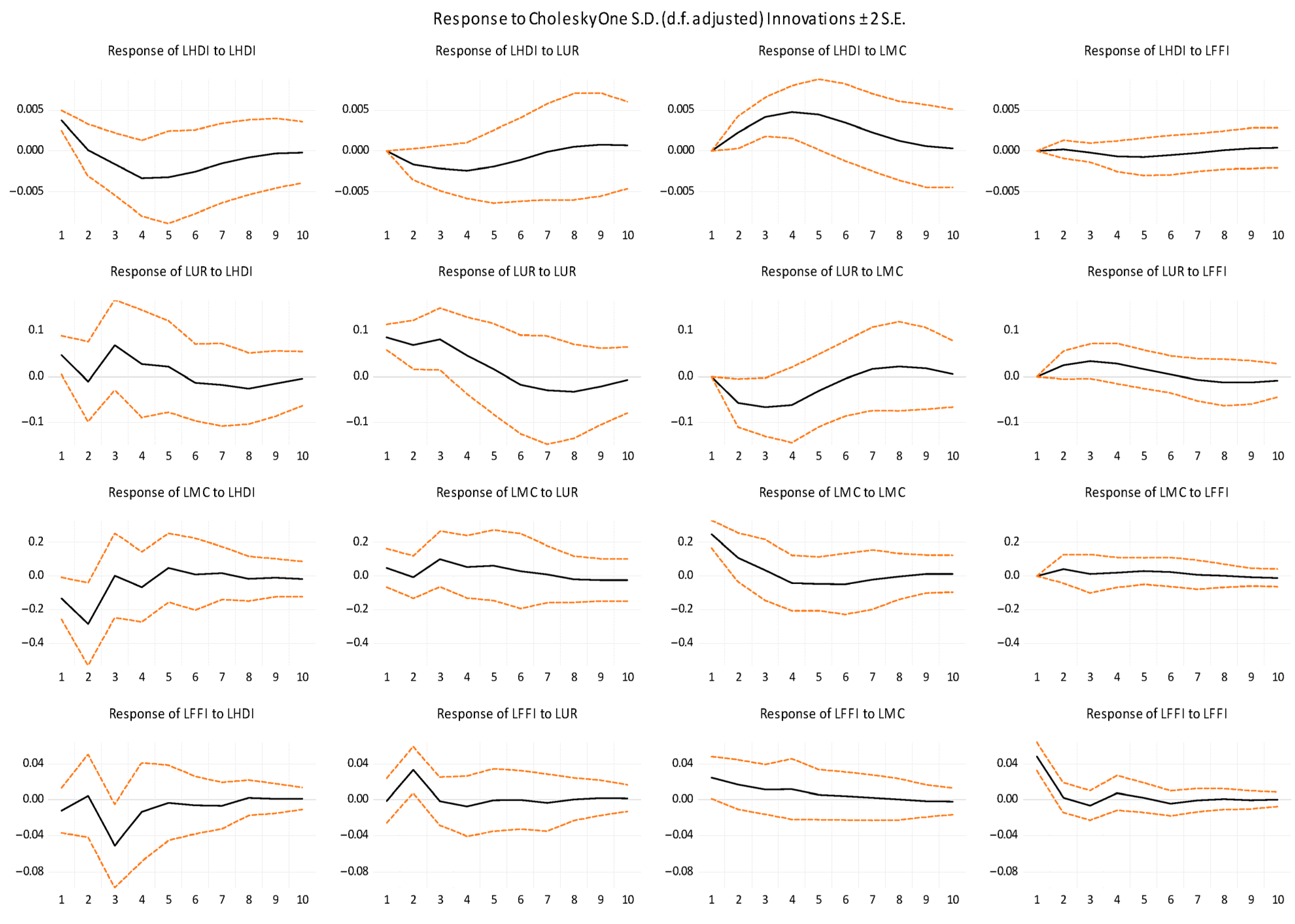
Figure 4 illustrates how one variable reacts to variations in another variable by means of the Cholesky IRFs. In most cases, IRFs show that one variable responds significantly to shocks in another variable. Especially in column 4 of Figure 5, one can see that the responses of LHDI and LMC to LFFI are characterized by small fluctuations around the zero line, the shock effects dying out. The response of LMC to LFFI can suggest that changes in FFI have a relatively limited impact on MC. MC tends to remain relatively stable, with small fluctuations not strongly correlated with changes in financial freedom. The response of LHDI to LFFI suggests that changes in financial freedom alone are not sufficient to drive significant changes in HDI.

According to

Table A1. Variance decomposition.

Variable	Period	LHDI	LUR	LMC	LFFI
LHDI	1	100.00	0.00	0.00	0.00
	5	31.26	13.68	54.24	0.80
	10	30.89	12.51	55.57	1.01
	15	31.07	12.50	55.31	1.10
	20	31.08	12.50	55.29	1.11
LUR	1	23.01	76.98	0.00	0.00
	5	18.49	47.44	27.70	6.34
	10	19.14	47.43	26.87	6.55
	15	19.68	46.60	27.26	6.44
	20	19.71	46.58	27.25	6.44
LMC	1	21.49	2.88	75.62	0.00
	5	50.87	9.41	38.11	1.59
	10	49.63	10.22	38.23	1.90
	15	49.47	10.37	38.19	1.96
	20	49.42	10.49	38.19	1.97
LFFI	1	4.74	0.060	19.43	75.75

from Appendix A, in the short term, LHDI is explained only by its own shocks. The forecast variance error of LHDI is explained in the 20th period by LMC (55.29%), followed by LUR (12.5%) and LFFI (1.11%). The substantial influence of LMC on LHDI suggests that the stock market’s relation with HDI indicates the strong confidence of investors in the Romanian economy, bringing overall prosperity.

In the long run, LMC has the most important contribution to LUR (27.25%), followed by LHDI (19.71%) and LFFI (6.44%). The high percentage (27.25%) points out that MC is an influential factor of UR. Changes in MC influence investor’s confidence and, consequently, job creation and economic growth.

In the long run, the contribution of LHDI to LMC is the highest (49.42%), followed by LUR (10.49%) and LFFI (1.97%). A prosperous economy has a higher MC. The stability induced by a prosperous economy instills confidence in national and international investors. UR is an economic indicator reflecting the situation of the labor market. High unemployment has a direct impact on MC. Consumer spending decreases, leading to a decline in companies’ revenues and profits, causing a fall in stock prices.

LHDI, LUR, and LMC explain LFFI through their innovative shocks. Economic development, measured by HDI, can have a positive impact on FFI. It leads to more job opportunities, easier access to financial services and financial stability, components of FFI. MC measures the total value of the stock market. MC is indirectly connected to FFI by economic development. A higher MC reflects more investment opportunities, which can enhance financial freedom by increasing wealth through investment.

4.2. A Multiple Linear Regression Approach to Evaluating Financial Stability and Human Well-Being

The multiple linear regression model we constructed examines the impact of financial contagion on human well-being in Romania. Given the current state of knowledge in the field, our analytical approach is valuable for assessing complex relationships in this context.

Before constructing the multiple linear regression model, an important step in preparing the data for regression analysis is to conduct a summary statistics analysis. This analysis aims to understand the data, its distribution, variability, and the relationships between the variables that will be used in the regression. In other words, summary statistics allow us to describe the data in straightforward terms, such as the mean, median, minimum, maximum, standard deviation, skewness, kurtosis, and so on. These measurements provide an overview of the central values, variability, and shape of the data distribution.

Summary statistics, including tests such as Jarque–Bera or Shapiro–Wilk, can help us assess whether the data follows a normal distribution. This is important for regression methods that assume a normal distribution of errors. By examining the correlations between the independent variables and the dependent variable, we can gain an initial understanding of potential regression relationships. Furthermore, summary statistics can reveal data issues, such as missing values or inconsistencies. Proper data cleaning is essential before creating a regression model.

Table 10. Summary statistics.

Statistics	GDP	HDI	VOL	BET-FI
Mean	7074.28	0.79	11.07	33,930.07
Median	6860	0.79	11.89	30,283.31
Maximum	10,110	0.82	16.93	78,669.68
Minimum	4350	0.72	4.08	6015.22
Std. Dev.	1670.04	0.02	3.65	18,307.93
Skewness	0.15	−1	−0.4	0.58
Kurtosis	2.13	2.88	2.34	2.99
Jarque–Bera	0.73	3.54	0.95	1.2
Probability	0.69	0.17	0.62	0.54

presents the summary statistics results for the variables to be used in the regression model. We observe that for the variable GDP, skewness has a value of 0.15, indicating a slight positive skewness (a longer right tail). For HDI, skewness is −1.00, indicating negative skewness (a longer left tail), suggesting that the data are skewed towards smaller values. For VOL and BET-FI, skewness is close to zero, indicating relatively low skewness. For all variables, Kurtosis is less than 3, suggesting that the data distribution is flatter (platykurtic) than a normal distribution, meaning there are fewer data points in the distribution tails.

The Jarque–Bera test is a test of data normality. The higher the value, the less likely the data follow a normal distribution (Gel and Gastwirth 2008). In the case of GDP, Jarque–Bera has a value of 0.73 with a probability of 0.69, suggesting that the data is approximately normally distributed. For HDI, the value is 3.54, with a probability of 0.17, indicating a significant deviation from normality. For VOL and BET-FI, the values are lower, indicating that the data are closer to a normal distribution. The probability associated with the Jarque–Bera test shows how likely the data is to follow a normal distribution. The lower the probability, the less likely the data is to be normal. While the probability is relatively high for GDP, it is lower for HDI, indicating a significant deviation from normality. For VOL and BET-FI, the probabilities are higher, suggesting a closer resemblance to a normal distribution.

The multiple linear regression model could help quantify how these variables influence human well-being in Romania and identify specific relationships among them. By evaluating these effects, our study can provide a better understanding of how financial contagion can impact people’s lives and contribute to the development of strategies and policies to safeguard human well-being in the face of financial risks.

Given the different units of measurement of the selected variables for the MLR model, we logarithmically transformed all the data. This process is a common technique used in data analysis to transform them into a suitable form to rectify the asymmetry, stabilize the variance, address the issue of data scaling, and transform proportion data. To ensure the stationarity of the time series data used, non-stationary data were transformed into stationary data using the logarithm transformation technique (Metcalf and Casey 2016). This helps in reducing the large differences between the values in the time series, making it easier to observe underlying trends or patterns. This is particularly useful for data with high variations or exponential growth trends. To perform model estimation, we utilized RStudio software (version 2023.09.1+494, developed by Posit, PBC), following a sequence of steps: data loading into the system, defining the dependent and independent variables, standardizing the dataset to establish a common metric, executing the multicriteria regression within the system, scrutinizing the results through the assessment of critical indicators like $R^2$, t-Statistic, or p-value, and subsequently interpreting the outcomes.

In

Table 11. Augmented Dickey–Fuller test.

Variables	Dickey–Fuller	p-Value
LGDP	−3.85	0.03
LHDI	−3.57	0.01
Lvol	−5.66	0.01
LBETFI	−3.82	0.03

, the ADF test was performed using the adf.test function in R Studio (Mushtaq 2011; Jalil and Rao 2019). Considering the p-value, which is lower than the significance level of 0.05, the data series are stationary.

It’s important to highlight that in the tables that follow, the values presented are rounded to two decimal places. However, when it comes to the mathematical equations based on these results, the coefficients will include all decimal points. In the output of

Table 12. Multicriteria linear regression output.

Residuals
Min	1Q	Median	3Q	Max
−0.095	−0.036	−0.007	0.036	0.151
Coefficients	Estimate	Std. Error	t-value	Prob.
(Intercept)	9.82	0.33	29.51	4.80 × 10−16 ***
LHDI	5.73	0.43	13.30	2.03 × 10−10 ***
Lvol	−0.13	0.03	−3.48	0.00 **
LBETFI	0.06	0.02	2.34	0.03 *
Performance metrics of MLR
Residual standard error	0.06 on 17 degrees of freedom
Multiple R-squared	0.94
Adjusted R-squared	0.93
F-statistic	100.7 on 3 and 17 DF
p-value	5.024 × 10−11

, “***” signifies that the p-value is extremely low (less than 0.001), “**” indicates a p-value less than 0.01, indicating a moderately high level of statistical significance, and “*” indicates a p-value less than 0.05, suggesting statistical significance, but at a lower confidence level.

Following the analysis of multiple linear regression (MLR) results from Table 12, we can draw the following conclusions:

➢

The intercept is 9.82 with an extremely low p-value, indicating its significance in the model. It represents the GDP value when all other independent variables are zero.

➢

The coefficient for LHDI is 5.73, with a t-value of 13.30 and a very low p-value, suggesting a significant relationship between the level of human development (HDI) and GDP. With a positive coefficient, an increase in HDI is associated with a significant increase in GDP.

➢

The coefficient for Lvol is −0.13 with a t-value of −3.48 and a very low p-value, indicating a significant relationship between transaction volume (Lvol) and GDP. With a negative coefficient, an increase in transaction volume is associated with a significant decrease in GDP.

➢

The coefficient for LBETFI is 0.06, with a t-value of 2.34 and a p-value of 0.03, suggesting a significant relationship between the BET-FI index and GDP. With a positive coefficient, an increase in the BET-FI index is associated with a significant increase in GDP.

Performance metrics of the model indicate a satisfactory explanation of GDP variability:

➢

Residual standard error: It measures how closely predicted values align with actual values. A low standard error indicates a good fit of the model to the data.

➢

Multiple R-squared: It stands at 0.94, indicating that approximately 94% of the variance in GDP is explained by the independent variables in the model.

➢

Adjusted R-squared: This value is 0.93, suggesting that the model fits the data well and that the independent variables significantly contribute to explaining the variance in GDP.

➢

F-statistic: A high F-statistic and low p-value indicate the overall significance of the model.

➢

p-value: Low p-values for each coefficient suggest the significance of all independent variables in the model.

In conclusion, the results indicate a significant relationship between HDI, transaction volume, the BET-FI index, and GDP. The coefficients and model statistics provide insights into the direction and significance of these relationships.

Regarding model validation, we conducted a series of additional analyses. Firstly, we examined the model residuals (Ye and Liu 2023; Wagner 2023) to ensure that they meet the assumptions of multiple linear regression.

To examine the model’s residuals, we used four methods (Arkes 2019): the residuals vs. fitted plot, normal Q-Q plot, scale-location plot, and residuals vs. leverage plot. The circles represent the residuals for each observation in the multiple linear regression model. The numeric values next to the circles represent observation identifiers or indices. The red curve represents the multiple linear regression line. According to Figure 5, Residuals vs. Fitted Plot is used to check linearity and homoscedasticity. In an ideal situation, residuals should be randomly distributed around the horizontal line at zero without a specific pattern. If you observe a distinct pattern or if residuals seem to spread as predicted values increase, this may indicate a violation of linearity or heteroscedasticity. The normal Q-Q plot helps assess the normality of residuals. In an ideal situation, points should follow a straight line. Deviations from the line suggest that residuals may not be normally distributed. Deviations at the ends of the Q-Q plot indicate possible outliers. Scale-Location Plot is used to check homoscedasticity and identify the presence of outliers. It is similar to the residuals vs. fitted values plot, but focuses on the distribution of residuals concerning predicted values. In a homoscedastic model, the distribution of residuals should be relatively constant across the entire range of predicted values. If you observe a pattern, it may indicate heteroscedasticity. Residuals vs. Leverage Plot helps identify influential data points (outliers). Points located far from the center of the plot (with high influence) can significantly impact the regression model. It is essential to check for observations with high influence and, if necessary, decide whether to exclude them from the analysis. These graphical methods aid in assessing the model’s assumptions and identifying potential issues in the regression analysis. Considering the observed distributions, we cannot definitively confirm or refute linearity and homoscedasticity. At this point, the decision was made to retain all variables as initially defined and incorporated into the MLR model.

Next, we will test the collinearity of the independent variables, as this can affect the interpretation of the coefficients. We have employed both the correlation matrix (Table 11) and the Variance Inflation Factor (VIF) (Marcoulides and Raykov 2019) values.

We can observe in

Table 13. Correlation matrix.

Variables	LBETFI	Lvol	LHDI
LBETFI	1	0.46	0.57
Lvol		1	0.27
LHDI			1

that the LBETFI and Lvol have a correlation coefficient of 0.46, suggesting a moderate positive correlation between the logarithm of the BET-FI index and the logarithm of transaction volume. When one increases, the other tends to increase as well, but the correlation is not very strong. Lvol and LHDI have a correlation coefficient of 0.27, indicating a relatively weak positive correlation between the logarithm of transaction volume and the logarithm of the Human Development Index (HDI). This suggests that there is a tendency for higher transaction volume to be associated with higher HDI, but the relationship is not very strong. LBETFI and LHDI have a correlation coefficient of 0.57, indicating a moderate positive correlation between the logarithm of the BET-FI index and the logarithm of the Human Development Index (HDI). This suggests that as one of these variables increases, the other tends to increase as well, and the correlation is moderately strong.

Variance Inflation Factor (VIF) values are used to assess the collinearity among the independent variables in your regression (Marcoulides and Raykov 2019). The higher the VIF, the greater the collinearity. Typical VIF values are under 5. According to

Table 14. Variance Inflation Factor (VIF) analysis.

Variables	VIF_Values
LBETFI	1.76
Lvol	1.27
LHDI	1.29

, for the LHDI variable, the VIF is 1.49. This indicates relatively low collinearity with the other independent variables. With a VIF below 5, there is not a significant collinearity for this variable. For the Lvol variable, the VIF is 1.27. This also suggests low collinearity with the other independent variables. A VIF under 5 for Lvol indicates that there is no significant collinearity for this variable. For the LBETFI variable, the VIF is 1.76. This VIF also demonstrates relatively low collinearity with the other independent variables. A value below 5 indicates that this variable does not exhibit significant collinearity. According to Table 14, the results suggest that collinearity among the independent variables in the model is low, meaning that they do not significantly affect the model’s ability to estimate the correct coefficients for each independent variable. This supports the robustness of our multiple linear regression model.

Continuing further, to identify whether there are cointegration relationships among our time series, especially to assess if the variables are integrated at the same order and if there are long-term equilibrium relationships among them, we employed cointegration analysis using the Johansen procedure (Johansen and Juselius 1990; Yussuf 2022).

The results obtained from the cointegration analysis using the Johansen procedure are presented in

Table 15. Cointegration analysis.

Johansen—Procedure
Eigenvalues (lambda)	0.93	0.72	0.29	0.04
Values of test statistic and critical values of test
	Test	10pct	5pct	1pct
$r\le 3$	0.08	6.50	8.18	11.65
$r\le 2$	6.76	15.66	17.95	23.52
$r\le 1$	31.10	28.71	31.52	37.22
$r=0$	81.83	45.23	48.28	55.43
Eigenvectors, normalized to first column (cointegration relations)
	y1.l2 (LGDP)	x1.l2 (Lvol)	x2.l2 (LHDI)	x3.l2 (LBETFI)
y1.l2 (LGDP)	1.00	1.00	1.00	1.00
x1.l2 (Lvol)	0.64	0.15	0.288	0.07
x2.l2 (LHDI)	4.88	−4.68	−9.12	−6.56
x3.l2 (LBETFI)	−0.39	−0.17	0.02	0.03
Weights W (loading matrix)
	y1.d (LGDP)	x1.d (Lvol)	x2.d (LHDI)	x3.d (LBETFI)
y1.d (LGDP)	−0.08	−0.47	−0.07	−0.02
x1.d (Lvol)	−1.32	2.64	−0.71	0.16
x2.d (LHDI)	−0.01	−0.01	0.02	0.00
x3.d (LBETFI)	−0.65	7.73	0.29	−0.40

. The eigenvalues (lambda) indicate that there are four eigenvalues or four cointegration relationships among the variables. The test and critical values show the number of significant cointegration relationships. In our case, $r\le 3$ and $r\le 2$ show the number of significant cointegration relationships, along with their associated critical values. The test values indicate that all four variables are cointegrated. The eigenvectors represent cointegration relationships, showing how the variables are correlated within these relationships. For instance, the values in the first column (y1.l2) depict the relationship between the variable LGDP and the other variables in each cointegration relationship. The loading matrix W displays the weights of each variable in each cointegration relationship. For example, in the first cointegration relationship, the LGDP variable is negatively influenced by the other variables, as indicated by the negative weights.

In order to analyze the long-term equilibrium relationships between the variables in our model, we will perform cointegration regression. Cointegration involves a statistical relationship that allows multiple time series to move together in the long term, even though they may have different short-term movements (Perron and Campbell 1994; Pascalau et al. 2022). The main idea behind cointegration regression is to model the long-term relationship between the series, considering that they may have stochastic trends or short-term fluctuations.

Overall, the results from

Table 16. Cointegration regression.

Variables	Coefficient	Std. Error	t-Statistic	Prob.
LHDI	5.83	0.37	15.63	0.00
Lvol	−0.16	0.03	−4.87	0.00
LBETFI	0.09	0.02	3.76	0.00
C	9.65	0.28	33.51	0.00
R-squared	0.94	Mean dependent var		8.83
Adjusted R-squared	0.93	S.D. dependent var		0.24
S.E. of regression	0.06	Sum squared resid		0.06
Long-run variance	0.00

suggest a strong cointegration relationship between the variables. The coefficients of LHDI, Lvol, and LBETFI are statistically significant, indicating their impact on the dependent variable (likely LGDP). The high R-squared value implies that the model explains a significant portion of the variance in the dependent variable. The intercept (C) is also highly significant, representing the constant term in the cointegration relationship.

These results suggest that there are significant cointegration relationships among the variables in our model, and cointegration analysis is crucial for understanding how these variables mutually influence each other over time. This outcome indicates that while the variables may be correlated over time, they are not merely dependent on each other. Instead, they evolve together over time due to a long-term relationship. In our context, cointegration implies that the LGDP, Lvol (volume of transactions), LHDI, and LBETFI have long-term relationships among them. This means that changes in one of these variables can have a significant and persistent impact on the others. In other words, they evolve together over time and are not independent of each other. Therefore, we can conclude that changes in GDP are related to changes in the volume of transactions, HDI, and the BET-FI index in the long run.

Our analysis results are significant, indicating that significant changes in GDP, which may be influenced by financial contagion, have a lasting impact on the other variables included in our study, such as human well-being measured by HDI. This can provide an important perspective on how financial events can affect economic development and human well-being in Romania. The cointegration among these variables may suggest a long-term interdependence between economic, financial, and human development aspects, thus contributing to a comprehensive understanding of how financial contagion can affect Romania in terms of sustainable development and human well-being.

4.3. Analyzing Financial Contagion Effects on Human Well-Being: The Role of the BET-FI Index and Altreva Adaptive Modeler

Considering the concept of financial contagion and our objective to analyze its effects on human well-being in Romania, the BET-FI index, which measures financial performance in Romania, was introduced into the multiple linear regression model. It reflects the evolution of listed stocks on the Bucharest Stock Exchange. By including the BET-FI index in our study, you can explore its relationship with other variables, particularly GDP and the Human Development Index (HDI), to gain a better understanding of how financial contagion can influence financial market performance. To do this, we utilized Altreva Adaptive Modeler software (version 1.6.0 Evaluation Edition) on BET-FI data to conduct a comprehensive analysis and evaluate its behavior and interactions with other economic and social indicators. The Altreva Adaptive Modeler (Chiriță et al. 2021; Marica 2015) is a powerful computational tool that brings a unique perspective to data analysis and modeling (Altreva Adaptive Modeler 2023). Its adaptability and versatility set it apart from conventional modeling tools. By incorporating this innovative software into our study, we gained the ability to explore complex relationships and analyze dynamic data patterns effectively.

The initial premises we considered regarding how financial contagion can be highlighted through the evolution of the BET-FI index are as follows:

➢

Price Effects: A financial crisis or a significant change in another financial market can lead to a decrease in stock prices in the Romanian financial market. Investors, especially foreign investors, may sell assets in the Romanian market, leading to a decrease in stock values and, consequently, the BET-FI index.

➢

Economic Effects: Financial contagion can impact Romania’s economy. A decline in financial markets can lead to reduced investor and consumer confidence. This can have a negative impact on economic growth, employment, and the overall development of the country.

➢

Trade Effects: If other countries are affected by a financial crisis, Romania’s exports and imports can be influenced. For instance, a decrease in the global demand for goods and services can negatively affect Romanian exports, which can lead to reduced economic activity and an impact on the BET-FI index.

➢

Foreign Capital Effects: Financial contagion can prompt foreign investors to withdraw capital from Romania or reduce new investments. This can affect the capital market and the BET-FI indicator.

➢

Psychological Effects: Sometimes, financial contagion has a psychological aspect. Investors may become more inclined to sell as they see global markets affected, leading to price reductions and a decline in the BET-FI index, even if economic fundamentals are sound.

These premises serve as a foundation for understanding how financial contagion and the BET-FI index may be interconnected.

The daily closing price data for the BET-FI index were retrieved from the Bucharest Stock Exchange website, maintaining the same time period as in the previous models, from 2000 to 2022.

The simulation conducted in Altreva Adaptive Modeler is carried out for 2000 agents/investors, each with an initial capital of 100,000 monetary units. This perspective can provide a framework for understanding how financial contagion affects a diverse range of investors in Romania. The simulation involves a large number of agents representing a diverse base of investors. This diversity may reflect the real-world scenario where various types of investors, such as retail, institutional, and foreign investors, participate in the capital market. Understanding how the behavior of these agents affects the index can offer insights into market dynamics.

An initial capital of 100,000 for each agent can help assess risk tolerance and exposure to different risks for various investors. A decline in the index can trigger different reactions among these investors, with some reducing their positions, while others might take advantage of the downturn. This can reflect how market volatility and risk aversion influence investor decisions. The simulation can capture investor sentiment, which can be influenced by news, economic events, or global financial developments. Sudden changes in the index can reflect shifts in market sentiment, which do not always align with fundamental economic factors.

Observing how changes in other financial markets or global economic events affect the simulated BET-FI index can provide insights into potential contagion effects. When agents respond to external shocks, they can trigger chain reactions on the index, demonstrating how financial contagion can spread. The simulation reveals how the trading behavior of different agents influences market dynamics. Some agents may employ strategies such as trend-following, value-based investments, or contrarian trading, which can lead to diverse price movements in the index.

The Altreva Adaptive Modeler enables us to understand how various economic and financial indicators, such as the BET-FI index, interact with one another and evolve over time. The software’s adaptive nature allows it to adjust and refine models based on the changing data landscape, providing insights into the relationships between variables and helping us identify patterns and trends that might not be evident through traditional statistical methods.

With Altreva Adaptive Modeler, we have a comprehensive and holistic approach to analyzing financial contagion and its effects on human well-being in Romania. It empowers us to make informed assessments and predictions regarding the intricate dynamics between financial market behavior and broader socio-economic outcomes, contributing to a deeper understanding of sustainable development in the context of economic volatility.

In Figure 6, a time snapshot of the simulation results can be observed. The first graph tracks how the forecast line compares to real prices. It is evident that the forecast aligns well with trading prices, indicating the model’s strong capability to anticipate market behavior. Specifically, the yellow line represents the real prices of the BET-FI index. The red line represents the forecasted future prices based on the model employed. This forecast is calculated using historical data and the model’s algorithms. The white line is a notation or indication of decision points or actions. The signal can vary depending on the objectives of the analysis. For instance, a “Buy” signal could indicate an opportune moment to purchase stocks, while a “Sell” signal might suggest the right time to sell.

The Wealth Distribution chart suggests that most of the agents or investors in the simulation have wealth levels that cluster around the central value of 417,666. However, there are a few agents with significantly larger wealth levels, indicating that a small portion of investors hold a substantial share of the total wealth. This interpretation may also suggest that there are significant disparities in wealth distribution among investors, which can be relevant in the context of risk analysis or when studying the effects of financial contagion on the market. The substantial wealth of a small number of investors can influence market dynamics and the spread of financial contagion in the simulation.

The third graph, Buy-Sell Orders, shows the number of buy orders and sell orders placed on the market at the same time. The differences between the two lines (the yellow line—buy orders, and the red line—sell orders) indicate the imbalance between the demand (buying) and supply (selling) of financial assets. If the “Buy Orders” line is greater than the “Sell Orders” line, it may indicate an increased interest in buying, potentially leading to a price increase. Conversely, if the “Sell Orders” line is greater, it may suggest a higher interest in selling and possibly exert downward pressure on prices. The significant fluctuations observed indicate market volatility and potential changes in the prices of financial assets.

The VM Trades—VM Trades MA (100) chart compares the trading volume in the market (VM Trades) with the moving average (MA) of trading volume over a 100-day period. It is observed that VM Trades (yellow line) exhibits fluctuations both above and below the VM Trades MA (100) line (red line). When it crosses above the red line, it highlights an increase in short-term trading activity compared to the longer-term average. This could indicate a surge in short-term market activity. Conversely, when VM Trades falls below VM Trades MA (100), it may indicate a decline in trading activity compared to the longer-term average.

The Population Position graph reflects the position of the population of agents or investors at a given moment. When significant variations are observed in this position, it may suggest changes in the structure or composition of the agents within the simulation.

The Avg Genome Size graph shows the average size of the genome or characteristics of the agents in the simulated population. This graph can provide insights into the diversity or complexity of agents in terms of the characteristics they use.

The Right–Wrong Forecasted Price Changes graph compares the number of correct forecasts with the number of incorrect forecasts of price changes. This analysis can offer a perspective on agents’ ability to accurately predict price movements.

The FDA–FDS (Trailing 100 bars) graph shows the difference between the FDA (First Difference Average) and FDS (First Difference Standard Deviation) indicators for the last 100 periods. This can indicate the volatility or stability of market dynamics.

The TS Wealth graph reflects the evolution of wealth or the total capital of agents over the course of the simulation. This graph can provide cumulative insights into the performance of agents in terms of profitability and risk exposure over time.

Based on the results presented in

Table 17. Trading simulator performance overview.

Status
Wealth at start	100.000
Wealth at end	190.906
Actual sub periods	11.63
FDA	51.8%
Return
Cumulative Return	90.91%
Compound Return/sp	5.72%
Cumulative Excess Return	−24.47%
Compound Excess Return/sp	−1.10%
$\beta$	0.26
Risk
Historical Volatility	11.20%
Value at Risk (VaR)	1.825
Maximum Draw Down	31.2%
Sharpe Ratio	0.51
Sortino Ratio	0.75
$\alpha$	3.9%
Risk-adjusted Return	4.75%
MAR Ratio	0.18

, the following discussion can be elaborated:

➢

The cumulative return of 90.91% indicates the total growth of the initial investment of 100,000 monetary units to 190,906 monetary units at the end of the period. This suggests a significant increase in investment over time.

➢

The compound return/sp of 5.72% indicates the average return over one-year sub-periods within the entire simulation. This shows how efficiently your investment performs in the short term.

➢

The cumulative excess return of −24.47% reflects the total return in excess of a benchmark or risk-free rate. In your case, it indicates a negative return compared to the benchmark or risk-free rate, suggesting that your investment may not have performed as well as the benchmark or risk-free rate.

➢

The compound excess return/sp of −1.10% shows the average excess return in one-year sub-periods within the simulation. This indicates how your investment has fared compared to the benchmark or risk-free rate in the short term.

➢

The Historical Volatility of 11.2% measures the historical volatility or risk associated with returns. The higher this value, the more volatile or risky the investment is.

➢

The Value at Risk (VaR) of 1.825 represents the maximum expected loss at a 95% confidence level. In other words, there is a 95% probability that the loss will not exceed this value during the simulation period.

➢

The maximum drawdown of 31.2% indicates the largest decline in the investment value compared to the previous peak during the simulation period.

➢

The Sharpe ratio of 0.51 evaluates the return in relation to the assumed risk. The higher the value, the more efficient the investment is in relation to the assumed risk.

➢

The Sortino ratio of 0.75 is a measure of return in relation to downside volatility. The higher the value, the better the investment performs concerning its downside volatility.

➢

The risk-adjusted return of 4.75% is the return adjusted for the assumed risk level. A higher value indicates greater efficiency in relation to the assumed risk.

➢

The MAR ratio of 0.18 represents the ratio of annualized return to the highest annualized decline, thus measuring the efficiency of the investment concerning its downside risk. A higher value suggests greater efficiency relative to downside risk.

Given that the analyzed period encompasses events with financial contagion effects, such as the economic crisis of 2007–2009, disruptions like the COVID-19 pandemic, and even the Russia–Ukraine armed conflict, we can argue that the growth recorded in investments despite the impact of financial contagion may suggest that, despite market volatility, Romania’s economy has managed to sustain sustainable growth. A historical volatility of 11.2% indicates a level of risk associated with your investment. This can be interpreted in the context of assessing the risks related to financial contagion on human well-being and sustainable development. With a Sharpe ratio of 0.51, the investment in the BET-FI index demonstrates efficiency concerning the assumed risk, implying effective risk management in the face of financial contagion. A Sortino ratio of 0.75 signifies adept handling of negative volatility, and this efficiency can be considered within the context of sustainable development and human well-being.

5. Conclusions and Policy Recommendations

In this paper, we applied the ARDL model to study the long- and short-run causality among HDI, UR, MC, and FFI for Romania during 2000–2022. We checked three hypotheses, H1, H2, and H3, which were confirmed to be true in the long run, as a result of the ARDL application. We found that in the long run, MC, and FFI positively impact HDI, while UR negatively impacts HDI. In the short term, a 1% increase in LFFI contributes to a 0.007% decrease in HDI. Balancing economic freedom with efficient financial regulation is important in order to minimize the risks associated with financial contagion.

Policymakers should put into action policies aimed at maintaining a degree of stability of the stock market of the Romanian economy. This encourages the formation of capital and upholds stability in the financial system.

Building upon the results obtained from the ARDL model, we retained the HDI variable and added transaction volume and the BET-FI index as independent variables. Through multiple linear regression, we modeled GDP as the dependent variable, contingent on the three aforementioned variables. The multiple linear regression model allowed us to quantify how these variables influence human well-being in Romania and to identify specific relationships among them. This analytical approach facilitated a deeper understanding of how financial contagion can affect people’s lives, contributing to the development of strategies and policies to safeguard human well-being against financial risks.

Incorporating the BET-FI index into the multiple linear regression model provided a more detailed perspective on Romania’s financial market performance. This index reflects the evolution of listed stocks on the Bucharest Stock Exchange and holds significance for our study. The relationship between the BET-FI index and other variables, such as GDP and the Human Development Index (HDI), can offer fresh insights into how financial contagion may impact financial market performance. This connection can be explored further to identify its influence on the economy and human well-being.

To complement our analyses, we utilized Altreva Adaptive Modeler software (version 1.6.0 Evaluation Edition). Analyzing the data related to the BET-FI index allowed for a comprehensive and detailed assessment of its behavior and interactions with other economic and social indicators. This powerful and versatile computational tool provides a unique perspective on data modeling, facilitating a more thorough understanding of these relationships. As for future research directions on this topic, we will continue the analysis and expansion of multiple linear regression models to delve deeper into the relationships between key variables and human well-being in the context of financial contagion. This can provide a solid foundation for developing strategies for managing financial risks and policies that ensure the stability of human well-being.

The purpose of the ARDL diagnostic tests in our study was not to run simulations or power analyses to determine type II error rates for the null hypotheses. Therefore, regarding future research directions, one of our concerns is related to the concepts of Type I and Type II errors within hypothesis testing. Type I errors occur when a null hypothesis is rejected when, in reality, it is true. If one sets the level of significance (alpha) at 0.05, for example, it means one is willing to accept a 5% chance of making a Type I error (rejecting a true null hypothesis). This is the threshold they have chosen to determine whether the relationship between the variables is statistically significant. Type II errors occur when a null hypothesis is accepted when, in reality, it is false. To calculate the power and Type II error rate for specific null hypotheses in ARDL model diagnostics, one would typically need to conduct power analyses or simulations, considering various factors, such as effect size, sample size, and significance level. These analyses help understand how likely the diagnostic tests are to correctly identify relationships or deviations from the null hypotheses when they exist.

In addition, we will further explore the impact of financial contagion on human well-being in a broader context, considering factors such as access to medical and educational services, living standards, and economic aspects. Regarding the use of the Altreva Adaptive Modeler software, in future analyses, we will employ it to assess and monitor the dynamics of the financial market and other economic variables. This tool can contribute to a deeper understanding of changes and trends in the economic environment.

Continuing research into the effects of financial contagion on human well-being and sustainable development, considering the complex interactions among financial factors and their impact on the quality of life in Romania. This interdisciplinary approach may bring new perspectives and effective solutions for managing financial risks and promoting sustainable human development.

References

1. Abdul Razak, Azila, and Mehmet Asutay. 2022. Financial Inclusion and Economic Well-Being: Evidence from Islamic Pawnbroking (Ar-Rahn) in Malaysia. Research in International Business and Finance 59: 101557. [Google Scholar] [CrossRef]
2. Adoms, Francis Uju, Henry Yua, Celestine S. Okaro, and Kelechukwu Stanley Ogbonna. 2020. Capital Market and Economic Development: A Comparative Study of Three Sub-Saharan African Emerging Economies. American Journal of Industrial and Business Management 10: 963–87. [Google Scholar] [CrossRef]
3. Altreva Adaptive Modeler. 2023. Available online: https://www.altreva.com/download.htm (accessed on 20 September 2023).
4. Androniceanu, Armenia, Irina Georgescu, Ionuț Nica, and Nora Chiriță. 2023. A Comprehensive Analysis of Renewable Energy Based on Integrating Economic Cybernetics and the Autoregressive Distributed Lag Model—The Case of Romania. Energies 16: 5978. [Google Scholar] [CrossRef]
5. Arkes, Jeremy. 2019. Regression Analysis: A Practical Introduction, 1st ed. London: Routledge. [Google Scholar] [CrossRef]
6. Assa, Jacob. 2021. Less Is More: The Implicit Sustainability Content of the Human Development Index. Ecological Economics 185: 107045. [Google Scholar] [CrossRef]
7. Asteriou, Dimitrios, and Stephen.G. Hall. 2015. Applied Econometrics, 3rd ed. Berlin: Springer. [Google Scholar]
8. Atsu, Francis, and Samuel Adams. 2023. Financial Development and Innovation: Do Institutions and Human Capital Matter? Heliyon 9: e19015. [Google Scholar] [CrossRef]
9. Batuo, Michael, Kupukile Mlambo, and Simplice Asongu. 2018. Linkages between Financial Development, Financial Instability, Financial Liberalisation and Economic Growth in Africa. Research in International Business and Finance 45: 168–79. [Google Scholar] [CrossRef]
10. Brown, Robert. L., James Durbin, and James M. Evans. 1975. Techniques for Testing the Constancy of Regression Relationships Over Time. Journal of the Royal Statistical Society: Series B (Methodological) 37: 149–63. [Google Scholar] [CrossRef]
11. Bucci, Alberto, Davide La Torre, Danilo Liuzzi, and Simone Marsiglio. 2019. Financial Contagion and Economic Development: An Epidemiological Approach. Journal of Economic Behavior & Organization 162: 211–28. [Google Scholar] [CrossRef]
12. Chiriță, Nora, Cristian Ciurea, and Ionuț Nica. 2021. An Analysis of Investment Decisions From ICT Industry in the Context of Behavioral Economy. Economic Computation and Economic Cybernetics Studies and Research 55: 159–76. [Google Scholar] [CrossRef]
13. Choi, Chi-Young, and Alexander Chudik. 2019. Estimating Impulse Response Functions When the Shock Series Is Observed. Economics Letters 180: 71–75. [Google Scholar] [CrossRef]
14. Choi, Insu, and Woo Chang Kim. 2023. Estimating Historical Downside Risks of Global Financial Market Indices via Inflation Rate-Adjusted Dependence Graphs. Research in International Business and Finance 66: 102077. [Google Scholar] [CrossRef]
15. Cristian, Elena Raluca, Alexandra Irina Dănciulescu, Carmen Dalia Țîrdă, and Anda Veronica Dan. 2022. The Relationship between the Human Development Index (HDI) and International Migration. Journal of Information Systems & Operations Management 16: 46–60. [Google Scholar]
16. Dickey, David A., and Wayne A. Fuller. 1979. Distribution of the Estimators for Autoregressive Time Series With a Unit Root. Journal of the American Statistical Association 74: 427. [Google Scholar] [CrossRef]
17. Du Plessis, Charmaine. 2023. Emotional Brand Communication on Social Media to Foster Financial Well-Being. Online Journal of Communication and Media Technologies 13: e202342. [Google Scholar] [CrossRef]
18. Ebrahimi Salari, Taghi, Ali Akbar Naji Meidani, Zeinab Shabani Koshalshahi, and Amir Abbas Ajori Ayask. 2022. The Threshold Effect of HDI on the Relationship between Financial Development and Oil Revenues. Resources Policy 76: 102537. [Google Scholar] [CrossRef]
19. Ella, Giscard Assoumou. 2014. International Crises, Characterization of Contagion and Social Well-Being in Developing Countries: A Theoretical Model. Theoretical Economics Letters 4: 72–77. [Google Scholar] [CrossRef]
20. Enders, Walter. 2014. Applied Econometric Time Series, 4th ed. Hoboken: John Wiley & Sons, Inc. [Google Scholar]
21. Engle, Robert, and Clive W. J. Granger. 1987. Co-Integration and Error Correction: Representation, Estimation, and Testing. Econometrica 55: 251. [Google Scholar] [CrossRef]
22. Frost, Thomas. 2017. Quantitative Economics. In Encyclopedia of Spectroscopy and Spectrometry, 3rd ed. Amsterdam: Elsevier, pp. 811–15. [Google Scholar] [CrossRef]
23. Gajurel, Dinesh, and Mardi Dungey. 2023. Systematic Contagion Effects of the Global Finance Crisis: Evidence from the World’s Largest Advanced and Emerging Equity Markets. Journal of Risk and Financial Management 16: 182. [Google Scholar] [CrossRef]
24. Garg, Nishant, Pushpendra Priyadarshi, and Ashish Malik. 2023. Towards An Integrated Framework Of Financial Well-Being: An Evolutionary Prespective. Academy of Management Proceedings 2023: 14473. [Google Scholar] [CrossRef]
25. Gel, Yulia R., and Joseph L. Gastwirth. 2008. A Robust Modification of the Jarque–Bera Test of Normality. Economics Letters 99: 30–32. [Google Scholar] [CrossRef]
26. Granger, Clive William John. 1981. Some Properties of Time Series Data and Their Use in Econometric Model Specification. Journal of Econometrics 16: 121–30. [Google Scholar] [CrossRef]
27. Gunay, Samet, and Gokberk Can. 2022. The Source of Financial Contagion and Spillovers: An Evaluation of the COVID-19 Pandemic and the Global Financial Crisis. PLoS ONE 17: e0261835. [Google Scholar] [CrossRef]
28. Hasan, Rezwanul, and Suborna Barua. 2015. Financial Development and Economic Growth: Evidence from a Panel Study on South Asian Countries. Asian Economic and Financial Review 5: 1159–73. [Google Scholar]
29. Ibinceanu, Cristina, Nicoleta Cristache, Catalina Dobre Răzvan, and Florescu Margareta. 2021. Regional Development in Romania: Empirical Evidence Regarding the Factors for Measuring a Prosperous and Sustainable Economy. Sustainability 13: 3942. [Google Scholar] [CrossRef]
30. Idenyi, Odo, Anoke Ifeyinwa, Onyeisi Samuel, and Chukwu Chibuzor. 2017. Capital Market Indicators and Economic Growth in Nigeria; An Autoregrssive Distributed Lag (ARDL) Model. Asian Journal of Economics, Business and Accounting 2: 1–16. [Google Scholar] [CrossRef]
31. Ionescu, Ștefan, Ionuț Nica, and Nora Chiriță. 2021. Cybernetics Approach Using Agent-Based Modeling in the Process of Evacuating Educational Institutions in Case of Disasters. Sustainability 13: 10277. [Google Scholar] [CrossRef]
32. Ionescu, Ștefan, Nora Chiriță, Ionuț Nica, and Camelia Delcea. 2023. An Analysis of Residual Financial Contagion in Romania’s Banking Market for Mortgage Loans. Sustainability 15: 12037. [Google Scholar] [CrossRef]
33. Jalil, Abdul, and Nasir Hamid Rao. 2019. Time Series Analysis (Stationarity, Cointegration, and Causality). In Environmental Kuznets Curve (EKC). Cambridge: Elsevier, pp. 85–99. [Google Scholar] [CrossRef]
34. Jin, Hui, and Mihajlo Jakovljevic. 2023. Fiscal Decentralization and the Human Development Index: A Cross-Border Empirical Study. Sustainability 15: 8784. [Google Scholar] [CrossRef]
35. Johansen, Søren. 1988. Statistical Analysis of Cointegration Vectors. Journal of Economic Dynamics and Control 12: 231–54. [Google Scholar] [CrossRef]
36. Johansen, Søren, and Katarina Juselius. 1990. Maximum Likelihood Estimation and Inference on Cointegration—With Applications to the Demand for Money. Oxford Bulletin of Economics and Statistics 52: 169–210. [Google Scholar] [CrossRef]
37. Jordà, Òscar. 2005. Estimation and Inference of Impulse Responses by Local Projections. American Economic Review 95: 161–82. [Google Scholar] [CrossRef]
38. Kassem, Jradi, El Chammay Rabih, Raad Georges, and Richa Sami. 2023. Effect of Human-Animal Interaction on the Well-Being and Quality of Life. L’Encéphale, S0013700623001380. [Google Scholar] [CrossRef] [PubMed]
39. Khattab, Ahmed, Mpabe Bodjongo Mathieu Juliot, and İhadiyan Abid. 2015. Financial Development, Financial Instability and Economic Growth: The Case of Maghreb Countries. International Journal of Economics and Financial 4: 1043–54. [Google Scholar]
40. Kilian, Lutz, and Helmut Lütkepohl. 2017. Structural Vector Autoregressive Analysis, 1st ed. Cambridge: Cambridge University Press. [Google Scholar] [CrossRef]
41. Kitamura, Kanji. 2022. Ethical Compatibility of Socially Responsible Banking: Comparing the Japanese Main Bank System with the USA. Research in International Business and Finance 62: 101686. [Google Scholar] [CrossRef]
42. Kolb, W. Robert. 2011. Financial Contagion. The Viral Threat to the Wealth of Nations. New Jersey: John Wiley & Sons, Inc. [Google Scholar]
43. Kwiatkowski, Denis, Peter C. B. Phillips, Peter Schmidt, and Yongcheol Shin. 1992. Testing the Null Hypothesis of Stationarity against the Alternative of a Unit Root. Journal of Econometrics 54: 159–78. [Google Scholar] [CrossRef]
44. Lütkepohl, Helmut, and Fang Xu. 2012. The Role of the Log Transformation in Forecasting Economic Variables. Empirical Economics 42: 619–38. [Google Scholar] [CrossRef]
45. Marcoulides, Katerina M., and Tenko Raykov. 2019. Evaluation of Variance Inflation Factors in Regression Models Using Latent Variable Modeling Methods. Educational and Psychological Measurement 79: 874–82. [Google Scholar] [CrossRef]
46. Mare, Codruța, Simona Laura Dragoș, and Ingrid-Mihaela Dragotă. 2019. The Impact of Human Development on the Romanian Life Insurance Market: A County Spatial Econometric Analysis. Cogent Business & Management 6: 1707609. [Google Scholar] [CrossRef]
47. Marica, Diana. 2015. Simulating an Evolutionary Multi-Agent Based Model of the Stock Market. Suceava: EcoForum, “Stefan Cel Mare” University of Suceava, Romania, Faculty of Economics and Public Administration—Economy, Business Administration and Tourism Department, Suceava, vol 4, pp. 1–42. [Google Scholar]
48. Menegaki, Angeliki N. 2019. The ARDL Method in the Energy-Growth Nexus Field; Best Implementation Strategies. Economies 7: 105. [Google Scholar] [CrossRef]
49. Metcalf, Leigh, and William Casey. 2016. Introduction to Data Analysis. In Cybersecurity and Applied Mathematics. Oxford: Elsevier, pp. 43–65. [Google Scholar] [CrossRef]
50. Mushtaq, Rizwan. 2011. Augmented Dickey Fuller Test. SSRN Electronic Journal, 1–19. [Google Scholar] [CrossRef]
51. Narayan, Paresh Kumar, and Russell Smyth. 2006. What Determines Migration Flows from Low-Income to High-Income Countries? An Empirical Investigation of Fiji–U.S. Migration 1972–2001. Contemporary Economic Policy 24: 332–42. [Google Scholar] [CrossRef]
52. Narula, Subhash C., and John F. Wellington. 1980. Linear Regression Using Multiple-Criteria. In Multiple Criteria Decision Making Theory and Application. Edited by Günter Fandel and Tomas Gal. Lecture Notes in Economics and Mathematical Systems. Berlin/Heidelberg: Springer, vol 177, pp. 266–77. [Google Scholar] [CrossRef]
53. Nica, Ionuț. 2020. Simulation of Financial Contagion Effect Using the NetLogo Software at the Level of the Banking Network. Theoretical and Applied Economics, Asociatia Generala a Economistilor Din Romania—AGER 3: 55–74. [Google Scholar]
54. Nica, Ionuț, and Nora Chiriță. 2020. Conceptual Dimensions Regarding the Financial Contagion and the Correlation with the Stock Market in Romania. Theoretical and Applied Economics, Asociatia Generala a Economistilor Din Romania—AGER 1: 75–86. [Google Scholar]
55. Nica, Ionuț, Daniela Blană Alexandru, Simona Liliana Paramon Crăciunescu, and Ștefan Ionescu. 2021. Automated Valuation Modelling: Analysing Mortgage Behavioural Life Profile Models Using Machine Learning Techniques. Sustainability 13: 5162. [Google Scholar] [CrossRef]
56. Nica, Ionuț, Nora Chiriță, and Camelia Delcea. 2023. Towards a Sustainable Future: Economic Cybernetics in Analyzing Romania’s Circular Economy. Sustainability 15: 14433. [Google Scholar] [CrossRef]
57. Nica, Ionuț, Nora Chirita, and Emil Scarlat. 2020. Approaches to Financial Contagion in the Banking Network: Theory and Case Studies. Chisinau, Republic of Moldova: LAP Lambert Academic Publishing. Available online: https://www.amazon.com/-/es/Ionu%C5%A3-NICA/dp/6202917970 (accessed on 25 September 2023).
58. Nkoro, Emeka, and Aham Kelvin Uko. 2016. Autoregressive Distributed Lag (ARDL) Cointegration Technique: Application and Interpretation. Journal of Statistical and Econometric Methods 5: 63–91. [Google Scholar]
59. Pascalau, Razvan, Junsoo Lee, Saban Nazlioglu, and Yan (Olivia) Lu. 2022. Johansen-type Cointegration Tests with a Fourier Function. Journal of Time Series Analysis 43: 828–52. [Google Scholar] [CrossRef]
60. Paun, Cristian, Radu Musetescu, Vladimir Topan, and Dan Danuletiu. 2019. The Impact of Financial Sector Development and Sophistication on Sustainable Economic Growth. Sustainability 11: 1713. [Google Scholar] [CrossRef]
61. Perron, Pierre, and John Y. Campbell. 1994. A Note on Johansen’s Cointegration Procedure When Trends Are Present. In New Developments in Time Series Econometrics. Edited by Jean-Marie Dufour and Baldev Raj. Heidelberg: Physica-Verlag HD, pp. 221–33. [Google Scholar] [CrossRef]
62. Pesaran, M. Hashem. 1998. An Autoregressive Distributed-Lag Modelling Approach to Cointegration Analysis. In Econometrics and Economic Theory in the 20th Century: The Ragnar Frisch Centennial Symposium. Edited by Steinar Strøm. New York: Cambridge University Press, pp. 371–413. [Google Scholar] [CrossRef]
63. Pesaran, M. Hashem, Yongcheol Shin, and Richard J. Smith. 2001. Bounds Testing Approaches to the Analysis of Level Relationships. Journal of Applied Econometrics 16: 289–326. [Google Scholar] [CrossRef]
64. Philips, Andrew Q. 2018. Have Your Cake and Eat It Too? Cointegration and Dynamic Inference from Autoregressive Distributed Lag Models. American Journal of Political Science 62: 230–44. [Google Scholar] [CrossRef]
65. Phillips, Jason. 2023. Determining Sustainability Using the Environmental Performance Index and Human Development Index—An Alternative Approach to the Environmental Human Index through a Holistic Quantitative Dynamic Framework. Science of the Total Environment 884: 163752. [Google Scholar] [CrossRef] [PubMed]
66. Phillips, Peter C. B., and Pierre Perron. 1988. Testing for a Unit Root in Time Series Regression. Biometrika 75: 335–46. [Google Scholar] [CrossRef]
67. Qiu, Jiaqi, Deyong Yu, and Ting Huang. 2022. Influential Paths of Ecosystem Services on Human Well-Being in the Context of the Sustainable Development Goals. Science of the Total Environment 852: 158443. [Google Scholar] [CrossRef]
68. Shrestha, Min B., and Guna R. Bhatta. 2018. Selecting Appropriate Methodological Framework for Time Series Data Analysis. The Journal of Finance and Data Science 4: 71–89. [Google Scholar] [CrossRef]
69. Singh, Ajit. 2011. Financial Globalisation and Human Development. Centre for Business Research Working Paper, Munich Personal RePEc Archive. WP421. Available online: https://mpra.ub.uni-muenchen.de/39048/1/MPRA_paper_39048.pdf (accessed on 28 September 2023).
70. Stock, James H., and Mark W. Watson. 2017. Twenty Years of Time Series Econometrics in Ten Pictures. Journal of Economic Perspectives 31: 59–86. [Google Scholar] [CrossRef]
71. Sumaryoto, Mirna Herawati, and Ambar Tri Hapsari. 2020. Analysis of Changes in the Unemployment Rate as a Result of the Human Development Index in Indonesia (Case Study 2010–2019). Journal of Economics and Business 3. Available online: https://ssrn.com/abstract=3739545 (accessed on 28 September 2023).
72. Țilică, Elena Valentina. 2021. Financial Contagion Patterns in Individual Economic Sectors. The Day-of-the-Week Effect from the Polish, Russian and Romanian Markets. Journal of Risk and Financial Management 14: 442. [Google Scholar] [CrossRef]
73. Vâlsan, Călin, Elena Druică, Zizi Goschin, and Rodica Ianole-Călin. 2023. The Perception of Economic Growth and the Romanian ‘Mioritic Syndrome’. Journal of the Knowledge Economy, 1–22. [Google Scholar] [CrossRef]
74. Wagner, Martin. 2023. Residual-Based Cointegration and Non-Cointegration Tests for Cointegrating Polynomial Regressions. Empirical Economics 65: 1–31. [Google Scholar] [CrossRef]
75. Wang, Hanjie, Jan-Henning Feil, and Xiaohua Yu. 2023. Let the Data Speak about the Cut-off Values for Multidimensional Index: Classification of Human Development Index with Machine Learning. Socio-Economic Planning Sciences 87: 101523. [Google Scholar] [CrossRef]
76. Ye, Tingqing, and Baoding Liu. 2023. Uncertain Significance Test for Regression Coefficients with Application to Regional Economic Analysis. Communications in Statistics—Theory and Methods 52: 7271–88. [Google Scholar] [CrossRef]
77. Yumashev, Alexei, Beata Ślusarczyk, Sergey Kondrashev, and Alexey Mikhaylov. 2020. Global Indicators of Sustainable Development: Evaluation of the Influence of the Human Development Index on Consumption and Quality of Energy. Energies 13: 2768. [Google Scholar] [CrossRef]
78. Yussuf, Yussuf Charles. 2022. Cointegration Test for the Long-Run Economic Relationships of East Africa Community: Evidence from a Meta-Analysis. Asian Journal of Economics and Banking 6: 314–36. [Google Scholar] [CrossRef]
79. Zhang, Yixin, and Zhijie Wu. 2022. Environmental Performance and Human Development for Sustainability: Towards to a New Environmental Human Index. Science of the Total Environment 838: 156491. [Google Scholar] [CrossRef]
Figure 1. The trend of variables.
Risks 11 00204 g001
Figure 2. Plot of CUSUM for coefficients’ stability of the ARDL model at 5% level of significance.
Risks 11 00204 g002
Figure 3. Inverse roots of the AR characteristic polynomial.
Risks 11 00204 g003
Figure 4. Impulse response functions.
Risks 11 00204 g004
Figure 5. Residuals analysis.
Risks 11 00204 g005
Figure 6. BET-FI simulation in the Altreva Adaptive Modeler (version 1.6.0 Evaluation Edition).
Risks 11 00204 g006