
Commodity Prices after COVID-19: Persistence and Time Trends


1
Faculty of Law, Business and Government, Universidad Francisco de Vitoria, E-28223 Madrid, Spain
2
Departamento de Ingeniería de Sistemas y Control, Universidad Nacional de Educación a Distancia (UNED), E-28040 Madrid, Spain
*
Author to whom correspondence should be addressed.
†
Current Address: Department of Financial Economics, Universidad Francisco de Vitoria, Crta. Pozuelo-Majadahonda, Km. 1800, Pozuelo de Alarcón, E-28223 Madrid, Spain.
‡
Current Address: Departamento de Ingeniería de Sistemas y Control, ETSI Informática, UNED, C/Juan del Rosal, 16, E-28040 Madrid, Spain.
Risks 2022, 10(6), 128; https://doi.org/10.3390/risks10060128
Submission received: 26 April 2022
/
Revised: 30 May 2022
/
Accepted: 6 June 2022
/
Published: 16 June 2022
(This article belongs to the Special Issue Frontiers in Quantitative Finance and Risk Management)
Abstract
:Since December 2019 we have been living with the virus known as SARS-CoV-2, a situation which has led to health policies being given prevalence over economic ones and has caused a paralysis in the demand for raw materials for several months due to the number confinements put in place around the world. Since the worst days of the pandemic caused by COVID-19, most commodity prices have been recovering. The main objective of this research work is to learn about the evolution and impact of COVID-19 on the prices of raw materials in order to understand how it will affect the behavior of the economy in the coming quarters. To this end, we use fractionally integrated methods and an Artificial Neural Network (ANN) model. During the COVID-19 pandemic episode, we observe that commodity prices have a mean reverting behavior, indicating that it will not be necessary to take additional measures since the series will return, by themselves, to their long term projections. Moreover, in our forecast using ANN algorithms, we observe that the Bloomberg Spot Commodity Index will recover its upward trend, increasing some 56.67% to the price from before the start of the COVID-19 pandemic episode.
JEL Classification:
C22; C45; E30; G10; G17; Q021. Introduction
The pandemic episode, caused by the SARS-CoV-2 virus, resulted in the paralysis of the demand for raw materials over several months due to the confinements and lockdowns that were imposed throughout the world, bringing about a collapse in prices.
Following the worst period of the COVID-19 pandemic, the demand for industrial metals, along with the demand for other raw materials, is now recovering. Many economic analysts (see Monge and Poza 2021; Monge and Gil-Alana 2021; among others) assume that a new cycle of economic growth will take place or, indeed, is already taking place, supported by various stimuli from governments and the main central banks.
The new projects put in place, or which will be launched to reform infrastructures (the Biden Administration in the United States, Recovery Funds in Europe, among others), will mean an increase in the demand for raw materials, with markets entering a new bullish cycle.
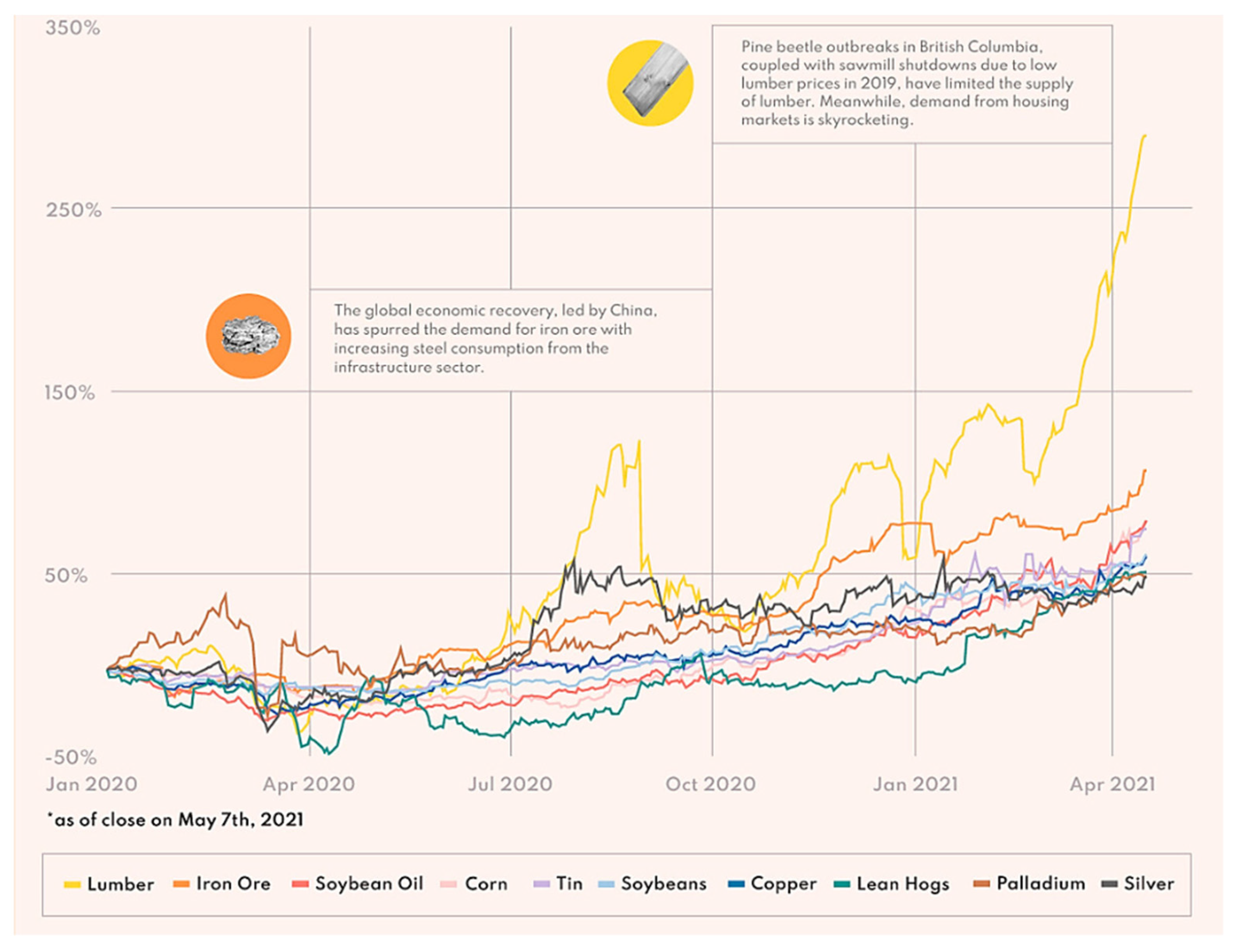
The beginning of the increase in the prices can already be seen in the various commodity markets. For example, the price of wood used for construction in the United States, such as pine or fir, has undergone strong price growth due to the high demand for houses and the shortage in the supply of this raw material. The price increase in wood futures is 63.5% this year and stands at 450%, approximately, compared to the price trough in 2020.
The rapid increase in the prices of raw materials underlines the importance of determining the evolution of prices and of analyzing the impact of this increase in economies, as well as the possible indirect effects deriving from it, such as the increase in the prices of basic necessities passed on to the final consumer. To this end, a study of the persistence of the current behavior of prices is required.
History has proven that market crises caused by the spread of disease often have a short-term impact. Following the detection of SARS on 12 March 2003, the Bloomberg Commodity Index fell 8% in the following two weeks, and it had fallen 4% by the time SARS had been brought under control.
In 2020, the Bloomberg Commodity Index fell by 9% in the month after the coronavirus was recognized by the WHO as a pandemic disease, dropping to 59.5 points in March 2020, and eventually recovering to 86 points in February 2021, which is a 44.5% increase.
Although last year’s rebound could be seen as a V-shaped recovery period, between January and April 2020, energy prices fell by nearly 60%, while metal and food prices fell by 15 and 10%, respectively. Metal prices rebounded in response to shocks to supply and a faster-than-expected recovery in China’s industrial activity, and food prices stabilized as concerns about restrictive policy measures faded. Goldman Sachs anticipated a new bull market in December 2020 because of the mismatch between supply and an expected increase in demand, caused by the greater maritime movement of medical supplies and the hope that vaccines against COVID-19 would return normality to the markets.
Due to the wide variety of assets included in the Bloomberg Commodity Index, volatility is very low, so events in specific industries may be prevented from having a significant impact.
According to (Erten and Ocampo 2013), the supercycles of raw materials are characterized by decade-long periods in which commodities are traded above their long-term price trend. The history of these markets shows that these supercycles last 20 to 70 years between peaks (Erdem and Ünalmış 2016). Some banks and market analysts are seeing signs of the start of a new supercycle, caused by the weakening of the dollar and central banks, along with the fiscal stimuli aimed at renewable energy and infrastructure spending.
The main objective of this article is to analyze the impact that the COVID-19 disease has had on commodity prices, recorded in the Thomson Reuters Eikon Bloomberg Commodity index, and to identify the possible appearance of a new commodity supercycle beginning after the 2020 health crisis, while studying, for this purpose, the trend and persistence of prices. To this end, various standard unit root tests and fractionally integrated methods based on ARFIMA (p, d, q) models were used. In addition, the results were supported by an Artificial Neural Network model using a Multilayer Perceptron (MLP) neural network for time series prediction. We examine the time series properties of commodity prices, from 2 January 1991 to 2 April 2021, using monthly data.
One of the interesting results is that, while focusing on the COVID-19 pandemic episode, we observe that both time series (the Bloomberg Spot Commodity Index and the Bloomberg Commodity Index Total Return) have a mean reversion behavior, indicating that it will not be necessary to take additional measures since the series will return, by themselves, to their long-term projections, but given the very wide confidence intervals (clearly due to the small sample sizes in some of the periods examined), we cannot reject Hypothesis I(1), in which the effect of the shock persists indefinitely. Thus, we observe an increase in the index price, from before the start of the COVID-19 pandemic episode, of 52.2%, using the Artificial Neural Network algorithm.
The rest of the paper is structured as follows. The next section briefly reviews the literature on the commodity prices and their cycles. In the following two sections, the data source and the methodology applied in the paper are detailed. Section 5 presents the main empirical results, while the final section shows the main conclusions of this work.
2. Literature Review
2.1. Commodity Prices
(Marshall 1890) describes the functioning of the commodity markets, how supply and demand determine the price, with buyers and sellers as the main actors, and how the market demand curve is determined by the consumer demand curves. When the supply of the good is equal to the demand, this is called the equilibrium price; however, we are dealing with a competitive market in which each economic agent considers that the price is beyond their control.
In recent decades, the evolution of commodity prices has been the subject of a recurrent debate. The growth of the world economy has also stimulated the growth of commodity markets, while supply is less and less able to adapt to changes in demand, as access to resources becomes more expensive. As supply becomes increasingly insensitive to demand, a small change in this demand can lead to significant price changes.
Whether the spot or futures market is the focus of price discovery in commodity markets has been widely discussed in the literature, with (Stein 1961) arguing that the spot and futures prices of a commodity are determined simultaneously. (Garbade and Silber 1983) developed a model of simultaneous price dynamics, while (Cox et al. 1981), (Jarrow and Oldfield 1981), and (Richard and Sundaresan 1981) argued that a futures contract can be thought of as a series of one-day spot contracts, in which there is a profit or loss on each day of a new contract.
(Pindyck 2004) studies how commodity markets tend to experience high levels of volatility, which can affect the trading strategies adopted by investors. The volatility of commodity prices has also been considerably higher since the beginning of the century. Although droughts, floods, labor strikes, and export restrictions have influenced short-term volatility, it would seem that a more structural supply problem can be observed, which affects long-term volatility.
Until the end of 1990, for 10 years, the prices of raw materials increased until a peak in 2008, by which time they tripled the levels of 1998 (Jacks 2013). During that period, there was a debate about the influence of roles of fundamentals, against speculation, that drove prices to those highs.
Along these lines, (Erdem and Ünalmış 2016) write that, while the majority of raw material prices had undergone a general downward trend from the 1960s to the early 2000s, between 2002 and the peak before the 2007 crisis, prices tripled. In response to the crisis, there was a drop in prices, with a recovery in 2011, followed by a further drop in 2015. They also show that energy prices increased almost five times between 1998 and 2008. Subsequently, prices fell in 2009 and 2010 in response to the global financial crisis, followed by a rapid recovery in 2011 and 2012. However, prices then fell rapidly, and in 2015, they barely reached half the price registered in 2012.
(Jacks and Stuermer 2020) write that, after the peak in 2008, prices went in the opposite direction, losing approximately 50% of their value.
(Erten and Ocampo 2021) study how, in 2020, after the initial impact of the pandemic, the gradual lifting of restrictions on mobility, as of the second quarter (Q2), and the economic stimulus packages boosted the recovery of activity and, therefore, led to an increase in the demand for raw materials—particularly those linked to the economic cycle—raising the possibility that we are facing a new supercycle in raw materials. Figure 1 reveals the impact suffered by raw materials throughout the first year of the pandemic.
2.2. Supercycles
In the literature, supercycles are defined as movements with periods of between 20 and 70 years, while being the most important cycles in current economic dynamics, among the Juglar, Kuznets, and Kondratiev cycles. (Jadevicius et al. 2017). (Juglar 1889) described the presence of short cycles as lasting between 8 and 11 years. (Kondratiev 1925) formulated, for the first time, the basic principles of the theory of supercycles, which reflect large variations in the prices of raw materials, industrial production, and foreign trade in periods of 40 to 60 years.
(Kuznets 1940) presents long-term cycles of 25 years, coinciding with the life cycles of innovations, which follow a cycle of medium duration.
(Radetzki 2006) identifies three booms in commodities. Based on the analysis of these booms, there is the first one in the early 1950s, then one in 1970, and, subsequently, in 2003. In 2012, (Cuddington and Zellou 2012) conducted research on supercycles in other commodities, while (Erten and Ocampo 2013) identified the magnitude and duration of supercycles in commodity prices, attributing to both the strong global growth of the economies and the last supercycle.
(Pedreira and Miguel-Angel 2012) explain that not all raw materials show a similar evolution in terms of supercycles, while energy products, with oil and metals as protagonists, represent the groups with the highest growth of prices from a long-time perspective. Meanwhile, primary industrial and food products show a marked decline. This divergence can be explained by the momentum in the price of energy and metals in the last 20 years due to global growth, driven by an intense use of raw materials linked to energy, metals, and their derivatives, by emerging countries in the early 1990s.
(Jacks 2013) conducted an investigation that aimed to gain an understanding of the long and medium-term trend in raw material prices, concluding that raw material prices have been increasing since 1950.
Since the beginning of the 21st century, the rise in the prices of most raw materials has been considerable; however, it must be borne in mind that, between the mid and late 1990s, these types of products fell to their lowest price levels in decades, including historical lows in some cases.
The studies identify the presence of long and short duration cycles, caused by the dynamics of supply and demand in the markets, while being highly influenced by the accelerations in economic growth that have occurred throughout history.
The ascents of the supercycles are characterized by being prolonged, although they may suffer a short recession. The recessions appear to be prolonged with weak and short recoveries, which can cause severe depressions, such as those that occurred after the years 1929 or 2008. An explanation for these cycles encompasses various factors, including development and innovations, exploitation of resources, technical modifications, or fluctuations in production.
2.3. Supercycle Analysis Methods
A major topic of discussion in applied economics is the long-term behavior of real commodity prices, especially if these series have a stationary trend or contain a unit root.
(Deaton and Laroque 1995) explained that, because storage cannot be negative, commodity prices are inherently non-linear.
In 1999, (Barkoulas et al. 1999) tried to provide evidence of long memory for the prices of commodity futures contracts that were traded on major U.S. exchanges. They compare it with the presence of fractional dynamics, in futures prices, for varieties of major foreign currencies and U.S. stock indices. They use fractional models investigated by (Mandelbrot 1977; Granger and Joyeux 1980; Hosking 1981; as well as Geweke and Porter-Hudak 1983). From a single parameter, known as the fractional differentiation parameter, the long-term dependence of these models is captured. The spectral regression method suggested by (Geweke and Porter-Hudak 1983) was used to carry out the tests.
(Lien and Tse 1999) examine, in their article, the performance of various hedge indices, using futures data from the NSA, along with the ARFIMA-GARCH approach, the EC model, and the VAR model. This analysis identifies the prevalence of a fractional cointegration relationship.
Using cointegration methodologies, (Kellard et al. 1999) developed a measure of relative efficiency for the presentation of fairness and efficiency tests in a variety of futures, financial, and raw materials markets. Their findings suggest that spot and futures prices are cointegrated with a slope coefficient, which is close to unity. This suggests that there are market inefficiencies in the sense that traders can use past information to predict spot price movements.
(Holt and Craig 2006) write about how that discrepancies between supply and demand for raw materials originate from non-linearities in prices, while Wang and Tomek (2007) argue that the primary terms of trade are better characterized by a stationary trend process.
There is a lack of studies on the non-linearities of the terms of trade, despite the fact that the real prices of the main categories of raw materials reflect periodic sharp spikes, followed by prolonged declines.
(Kilian 2009) used autoregressive models to decompose changes in oil prices, from which an extensive academic literature on oil prices since the 1970s has developed.
The study carried out by (Coakley et al. 2011) explores the impact of the time series properties of the spot futures basis and the cost of forward market bias carry-over. The main result is the existence of a robust long memory, even for the break-adjusted data, which implies that the cost-of-carry has a long memory and is something that the empirical results confirm using the interest cost as a proxy. These results suggest that forecast error has a long memory and is inconsistent with bias.
(Erten and Ocampo 2013) used the asymmetric Band–Pass Filter (BP) method of (Christiano and Fitzgerald 2003) for the identification of cycles in the different commodity price indices. The BP filter allows a time series to be broken down into different frequency components, which then identify the cycles at different commodity prices.
Using fractional integration techniques, (Gil-Alana et al. 2012) investigated the degree of persistence of various weekly and monthly agricultural prices. They saw that, when a structural break was taken into account, they found that, during the first subsamples, the series were stationary, although very persistent, with large autoregressive coefficients and with integration orders close to zero.
(Clavijo-Cortes et al. 2020) investigated whether a unit root process and nonlinearities can characterize the real prices of raw materials for six main primary goods by using a threshold autoregressive model of two regimes, without constraints, with an autoregressive unit root. They concluded that the terms of trade of non-energy raw materials are non-linear processes characterized by a unit root process.
2.4. The Economic Impact of COVID-19
The confinements imposed after the onset of the SARS-COV-2 virus pandemic resulted in the cessation of a large part of commercial activity, causing important changes in the economic situations of all countries. Thus, (So et al. 2021) studied the impact of the pandemic on financial market connectivity in Hong Kong, comparing its impact with crises from the previous 15 years. (Narayan et al. 2020) focused on the analysis of the government responses of the G7 countries, to the COVID-19 pandemic, on stock market returns and how governments tried to minimize the economic repercussions of the pandemic.
In addition to the consequences derived from the lockdowns, it is necessary to analyze the behavior of consumers during the pandemic. (Goolsbee and Syverson 2020) examined the drivers of the economic slowdown, concluding that the legal closure orders only represent a part of the massive changes in behavior.
In the agricultural field, (Ceballos et al. 2020) analyzed, from telephone surveys, the interruptions in agricultural production and food security due to COVID-19, thus analyzing the impact of the measures adopted in agriculture and farms, which remained reflected in the increase in derived products.
The literature about the economic consequences of the pandemic has been growing continually. The effects of the restrictions have been evident in many sectors, especially in the world financial markets, which were affected from the outset of the pandemic and also by a decrease in the efficiency of the markets during the outbreak, thus exerting an even greater effect on the Australian dollar (Aslam et al. 2020). This explains the increasing risk aversion on the part of investors in developed and emerging equity markets, especially during the pandemic (Fassas 2020), while (Just and Echaust 2020) examined the structural breaks in the returns of the stock market, focusing on three financial market indicators: expectations of volatility, correlation, and lack of liquidity during the COVID-19 crisis. Along the same lines, (Papadamou et al. 2020) investigated the impact of the pandemic on the time-varying correlation between stock and bond returns by using a panel data specification and wavelet analysis. Other studies focus on the analysis of the impact of the health crisis on cryptocurrencies, such as the one carried out by (James et al. 2021), in which they present new methods for the analysis of behavior in the dynamics of the cryptocurrency market types of currencies by studying 51 cryptocurrencies.
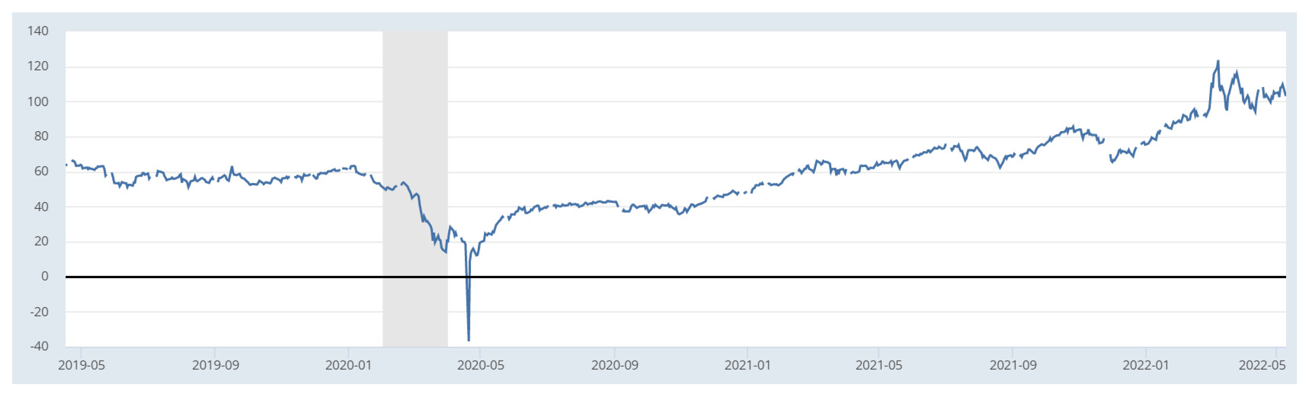
Much of the research focuses on how the health crisis and lockdowns have affected commodity prices, as many commodity and financial markets experienced a decline in performance during the pandemic, thus requiring the effects of the lockdown and the pandemic on the connection of markets to be examined (Adekoya and Oliyide 2020). Some of this research focuses, particularly, on the impact on oil prices, such as (Corbet et al. 2020), who prove the existence of indirect effects of volatility among energy-focused corporations during the COVID-19 outbreak, or (Akhtaruzzaman et al. 2020), who, in their study, show that oil-supplying industries benefit from positive shocks to oil price risk in general, while oil-using and financial industries react negatively. (Salisu et al. 2020) provide some preliminary estimates on the behavior of the oil stock nexus during the pandemic, in their study to analyze the response of oil and stocks to shocks, as reflected in the graph in Figure 2. In this graph, the evolution of the price of oil throughout the pandemic can be seen, the recessions in the United States are shaded, coinciding with an immediate drop in prices. The research carried out by (Sharif et al. 2020) focuses on the analysis of the connection between the recent spread of the COVID-19 virus, the shock of oil price volatility, the stock market, geopolitical risk, and the uncertainty of economic policy in the US.
For a complete analysis of the economic situation resulting from the health crisis, it is necessary to determine the impact of COVID-19 on gold and oil prices based on upward and downward trends. (Mensi et al. 2020), in their study, conclude that gold and oil have become more inefficient during the pandemic outbreak compared to the pre-COVID-19 period. Following this line, (Akhtaruzzaman et al. 2021b) investigate the role of gold as a hedging or safe haven asset in different phases of the pandemic.
All these studies show that there has been a significant financial contagion effect between China and its main trading partners during COVID-19 (Banerjee 2021). Research that coincides with that carried out by (Akhtaruzzaman et al. 2021a), in which they examine how this contagion occurs between China and the G7 countries, shows, as a result, that publicly traded companies in these countries experience a significant increase in the conditional correlations between their stock returns.
2.5. Multilayer Neural Networks in Commodity Forecasting
Having the ability to forecast the trend or price of stocks is one of the main goals of investors in the markets. Given the non-linear behavior of this type of economic variable since the 1990s, and thanks to the increase in the computing capacity of Artificial Neural Networks (ANN), new methods with great capacities for data processing have been proposed, achieving the creation of predictive models with greater precision than traditional statistical techniques (Villada et al. 2012).
The main characteristic of the ANNs—allowing the establishment of linear and non-linear relationships between the inputs and outputs of an algorithm—has proved useful in its application in high volatility markets, whose variables obey non-linear behavior in various areas of engineering, as well as in the electricity markets (García et al. 2008; Villada et al. 2011). One of the earliest extant reviews that successfully looked at a broad set of the applications of neural networks in finance is presented in (Trippi and Turban 1996). (Li and Ma 2010) present an updated review of these applications of predictions in stock markets, derivatives, foreign exchange, and financial crises.
(Haidar et al. 2008) presented a short-term forecasting model for crude oil prices based on a three-layer forward neural network. By testing various features as inputs, such as crude oil futures prices, the dollar index, gold spot price, and heating oil spot price, they showed that, with a suitable network design and an appropriate selection of training inputs, ANNs are capable of forecasting noisy time series with high accuracy.
A multilayer feedforward neural network was used by (Kulkarni and Haidar 2009) for the prediction of short-term oil price values, up to three days in advance, obtaining accuracy levels between 60% and 78%. In this study, special attention was paid to finding the optimal structure of the ANN model by testing various data preprocessing methods.
A review of 100 scientific publications dedicated to price forecasting in stock markets from different parts of the world, using neural networks and neuro-fuzzy networks, is presented by (Atsalakis and Valavanis 2009). All these works demonstrate the superiority of these intelligent computing techniques, with respect to conventional models, as far as better forecast accuracy is concerned.
(El-Henawy et al. 2010) also applied Neural Networks of the Multi Layer Perceptron (MLP) type to the prediction of stock market indices. From these reviews, the superiority in the performance of neural networks, with respect to econometric methods and other linear models, is highlighted.
The study by (Chen and Tanuwijaya 2011) compared the performance of models based on time series and fuzzy logic, with an algorithm also based on time series, but modifying the inputs for the variation in price and the sign of the trend. In its application to the Taiwan stock market index, it was found that the proposed model outperformed the forecast with AR, ARMA, and fuzzy logic models, in most cases.
(Sanchez et al. 2015) confirmed the superiority of neural networks over ARIMA models in predicting copper spot prices on the New York Commodity Exchange (COMEX), with ANNs showing better performance over the ARIMA model, along the same lines of some of the previous studies.
3. Data and Methodology
3.1. Dataset
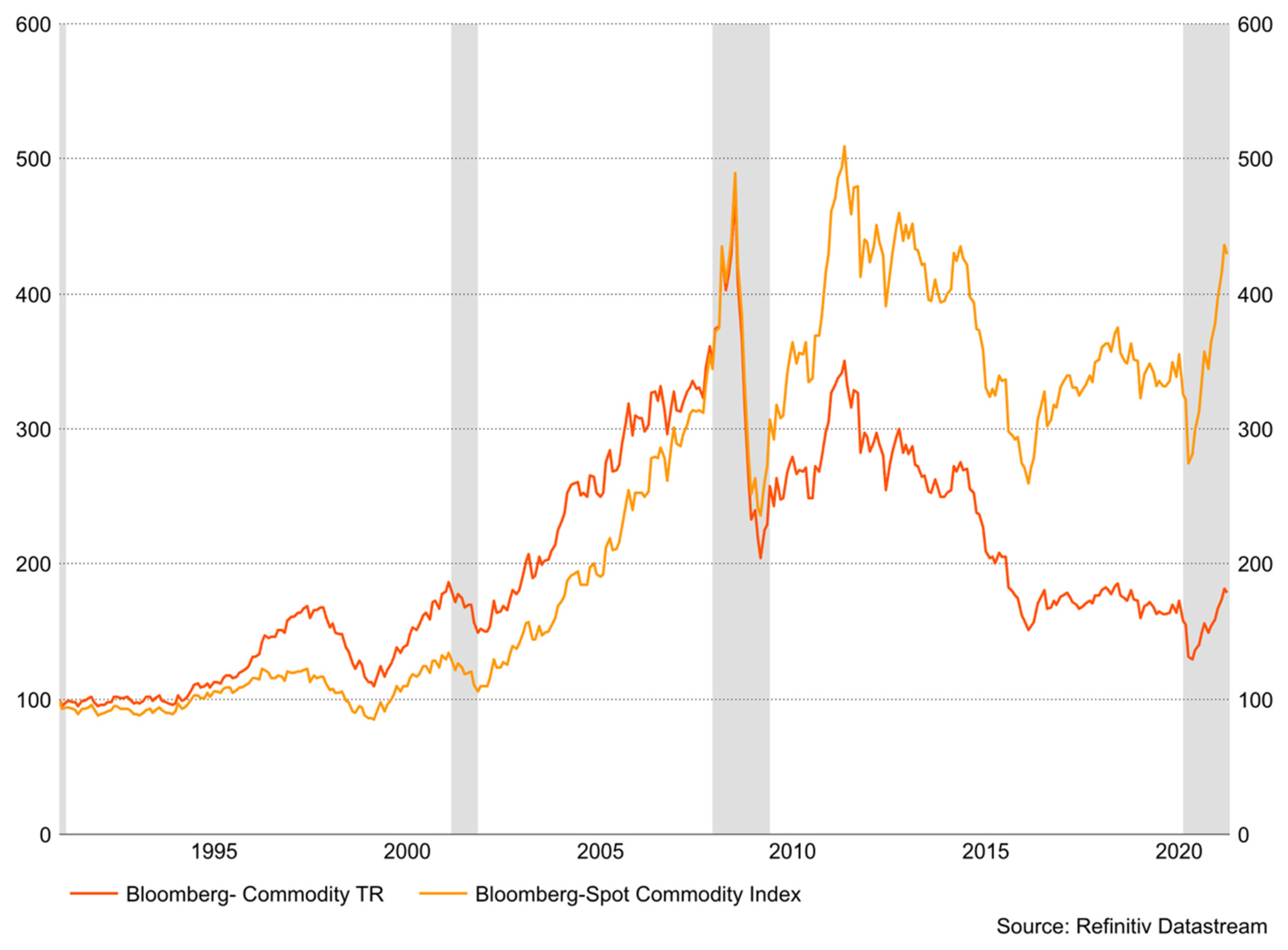
In this paper, we used the Bloomberg Spot Commodity Index and the Bloomberg Commodity Index Total Return, in monthly frequency, to carry out our analysis from 2 January 1991 to 2 April 2021. The data were obtained from the Thomson Reuters Eikon Database and are shown in Figure 3. Both indices represent certain commodities related to energy, livestock, softs, industrial metals, precious metals, and grains.
To take into account the various U.S. recessions, we have used the dates provided by the Federal Reserve Bank of St. Louis1.
We have also considered other disease outbreaks, such as Severe Acute Respiratory Syndrome (SARS), which, according to the WHO, began in November 2002 and ended in May 20042, Middle East Respiratory Syndrome (MERS), which began in September 2012 and is still currently active, and finally, we analyze COVID-19. To consider the coronavirus crisis (10th recession period), we have taken the start date indicated by (Hui et al. 2020) and the World Health Organization (WHO) and used figures up to the current available data.
The dates that we have used for our analysis are detailed in the following Table 1:
3.2. Unit Roots
Augmented Dickey Fuller (ADF) test, based on (Fuller 1976 and Dickey and Fuller 1979), has been used to know the stationarity of the data analyzed in this paper. Additionally, a non-parametric estimate of the spectral density of at the zero-frequency, based on (Phillips 1987 and Phillips and Perron 1988), and deterministic trend estimates, based on (Kwiatkowski et al. 1992; Elliott et al. 1996, and Ng and Perron 2001), have been used because they have a greater power of estimation.
3.3. ARFIMA (p, d, q) Model
To carry out this research and due to the lower power of unit root tests (see Diebold and Rudebush 1991; Hassler and Wolters 1994; and Lee and Schmidt 1996), we also employ fractionally integrated methods with the purpose of getting the time series to be stationary. We achieve this objective () by differentiating the time series with a fractional number.
Using a mathematical notation, a time series follows an integrated order process (and is denoted as ) if:
where refers to any real value, indicates to the lag-operator , and is a covariance stationary process I(0), where the behavior of the spectral density function shows, in the weak form, a type of time dependence where the function is positive and finite at the zero frequency.
It is said that xt is ARFIMA (p, d, q) when is ARMA (p, q). Thus, depending on the value of the parameter on (1), the reading of the results can be: xt is anti-persistent if d < 0 (see Dittmann and Granger 2002); when in (1), we say that the process is short memory I(0); with a high degree of association over a long time, we say that the process is long memory (d > 0); d < 1 means that the shock is transitory, and the series reverts to the mean; finally, when d ≥ 1, we expect that the shocks will be permanent.
We follow the methodology proposed by (Sowell 1992) instead of others (see Geweke and Porter-Hudak 1983; Phillips 1999, 2007; Sowell 1992; Robinson 1994, 1995a, 1995b; etc.), and to select the most appropriate ARFIMA model, we use the Akaike information criterion (AIC) (Akaike 1973) and the Bayesian information criterion (BIC) (Akaike 1979).
3.4. Forecasting with Artificial Neural Networks
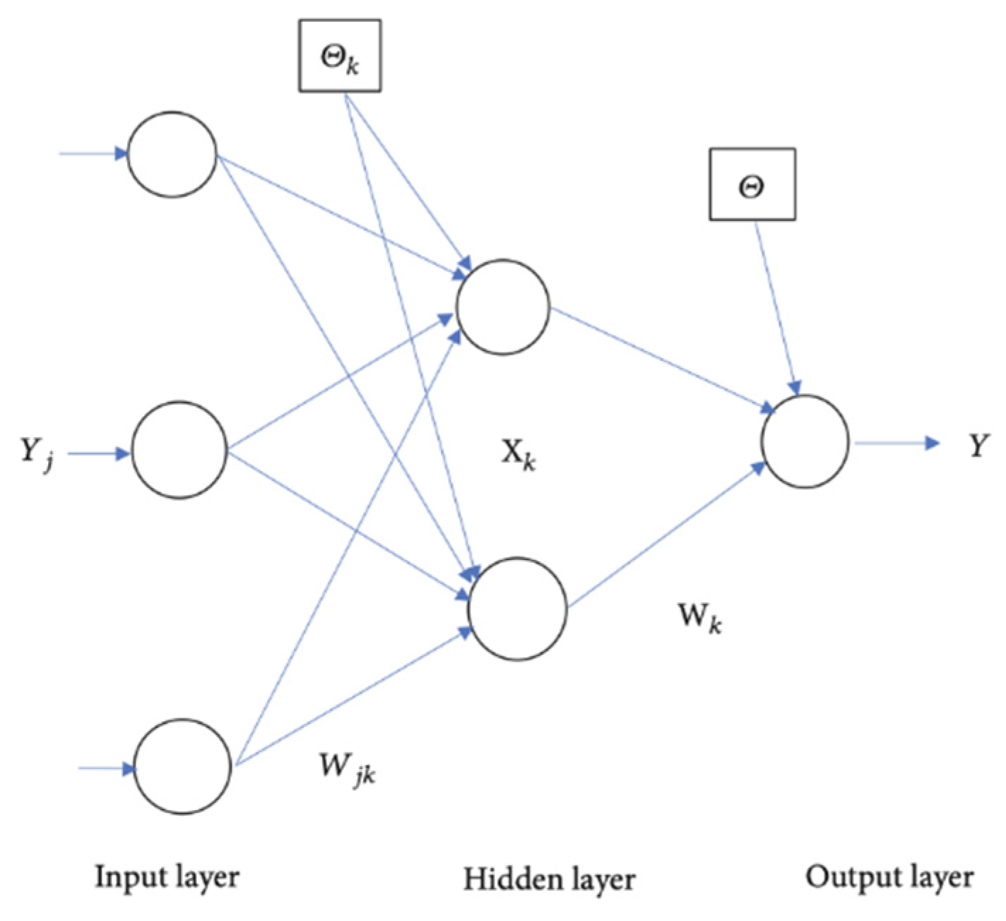
A neural network is characterized by the fact that its neurons are grouped in layers by levels, and there are three types of layers: input, hidden, and output (Zhang et al. 2020). In each layer, we have to consider the number of neurons, the training algorithm parameters, and the performance measure.
(Rumelhart et al. 1986), described that, in the input layer, there are neurons that are only responsible for receiving signals from outside, and they propagate this data to all neurons in the next layer, while the last layer acts as output, providing an output response for each input. Neurons in hidden layers perform non-linear processing of received inputs.
According to (Güler and Übeyli 2005), there is no general rule for finding the optimal number of hidden layers, and the most popular approach is trial and error.
The architecture of the neural network can be generalized as follows:
where represents the number of input nodes, the number of neurons in the hidden layer , and the number of neurons in the output layer.
(Fu 1994) wrote about how the neurons of one layer are connected with the neurons of the next layer. These connections are assigned a weight, which is calculated from the comparison between the result obtained in the output layer and the expected real result. This error propagates backwards and allows the weights to be adjusted during the training process. To control this process, a second group of data will be used, from which the model will be evaluated. The most widely used criterion is to reduce the mean square error between the result obtained and the expected real value.
According to Figure 4, represents the input vector denoted by ; the connection weight vector of the nodes of the input layer to the nodes of the hidden layer is represented by ; the vector of the neurons in the hidden layer is the , determined by the formula ; the connection weights of the nodes of the hidden layer to the output layer is represented by ; the unit output vector for the neural network with one output neuron is which is determined by the formula . Finally, is the bias value of the hidden layer nodes, and is the bias value of the output layer.
The application of artificial neural networks covers the prediction of problems in different areas of knowledge, such as biology, medicine, economics, etc. (Arbib 1995; Simpson and Brotherton 1995; Arbib et al. 1997), thereby obtaining excellent results, with respect to classical statistical models (de Lillo and Meraviglia 1998; Arana et al. 2003). The parallel processing capability allows neural networks to learn relationships between variables without the imposition of assumptions or constraints.
(Hinton and Salakhutdinov 2006) began to develop deep learning by showing that it was possible to train neural networks by properly initializing the weights in networks with a large number of deep layers, rather than with random values. This process began by training each of the layers in an unsupervised manner, and then, it continued with supervised training, using the resulting weights of the pre-trained layers as initial values.
(Glorot and Bengio 2010) proposed an efficient weight initialization scheme, commonly known as Xabier Initialization, with the ability to initialize weights without the need for unsupervised training. This has become the deep learning standard, and it has also demonstrated a great impact on training and improving accuracy with the choice of a nonlinear activation function. This led to a new line of research focused on finding adequate activation functions and, as a result, identified the Rectified Linear Unit (ReLU) (Jarrett et al. 2009; Nair and Hinton 2010; Glorot et al. 2011).
The data described in Section 3.1 are divided into a training set, consisting of 80% of the recorded data, and a test set (20%). This latter group will be used for model validation: checking that the result obtained is the expected one. This division is made following the study carried out by (Gholamy et al. 2018), in which they show that the best results are obtained using an 80–20 division, thus avoiding an overfitting of the network due to a lack of training data.
The forecasts obtained with the neural network are compared using the multiple regression technique. The predictive capacity for both methods is evaluated using the Mean Squared Error (MSE) and Root Mean Square Error (RSME) error measurement techniques.
4. Empirical Results
We have calculated the three standard unit roots tests to analyze the statistical properties of the commodity market.
Table 2 displays the results, which suggest that the original data are stationary I(1).
Using unit root methods in the time series, we conclude that we have to use the first differences, as we have verified that the data is non-stationary I(1). However, we use fractional alternatives, such as ARFIMA (p, d, q) models, due to the low power of the unit root methods, to study the persistence of the time series related to commodity spot prices.
To get the appropriate AR and MA orders in the model, we consider the Akaike information criterion (AIC; Akaike 1973) and the Bayesian information criterion (BIC; Akaike 1979)3.
For each time series, we show, in Table 3, the fractional parameter and the AR and MA orders obtained using (Sowell’s 1992) maximum likelihood estimator and taking into consideration .
We observe, from Table 2, that the Bloomberg Spot Commodity Index and Bloomberg Commodity Index Total Return have the same behavior. We also observe that the I(0) hypothesis cannot be rejected in the cases of the first recession in the United States and the SARS and MERS epidemic episodes, while for the second recession, this hypothesis is rejected in favor of a lower degree of integration.
Focusing on the COVID-19 pandemic episode, we observe that both time series have a mean reversion behavior, indicating that it will not be necessary to take additional measures since the series will return, by themselves, to their long term projections, but according to the confidence interval, we cannot reject Hypothesis I(1) where the effect of a shock persists indefinitely, due to the confidence intervals being very wide (clearly due to the small sample sizes in some of the periods examined).
Based on the results obtained up to this point, and in order to lend more accuracy and rigor to this study, we have also used advanced computational intelligence techniques, based on machine learning, to forecast the Bloomberg Commodity Indices listed previously.
We have used a Multi Layer Perceptron (MLP) neural network for time series prediction. This methodology presents interesting features, such as its nonlinearity or the lack of an underlying model (non-parametric model), to obtain the results. The MLP neural network is one of the most widely implemented neural networks based on the back-propagation rule where the errors are propagated through the network and allow the adaption of the hidden processing elements. In addition, the MLP has massive interconnectivity, which means that any element of a given layer feeds all the elements of the next layer, and it is trained with error correction learning.
To find out what the most accurate prediction model is and following (Mapuwei et al. 2020), we have used the Mean Squared Error (MSE) and Root Mean Square Error (RSME), as these are the evaluation methods used most in prediction methods with Machine Learning (see Barrow and Crone 2016b; Coulombe et al. 2020). The mean square error (MSE) is, by far, the most used cost function in regression problems. For a given observation ii, the squared error is calculated as the squared difference between the predicted value y^y^ and the actual value yy.
l(i)(w,b) = (y^(i) − y(i))2
The mean absolute error (MAE) consists of averaging the absolute error of the predictions.
The mean absolute error is more robust against outliers than the mean square error. This means that model training is less influenced by outliers in the training set (Taud and Mas 2018).
In Table 4, we present the results and the accuracy of the BSCI time series using an Artificial Neural Network (ANN) model until February 2022, due to the war between Russia and Ukraine. The results obtained are in line with the literature, which states that the most prominent machine learning technique used in time series forecasting is the Artificial Neural Networks, which obtains values very close to zero, indicating that this is the best model with which to predict the time series under examination.
We observe, from the results in Table 4, that the neural network model has an error rate (MSE) of 0.0005. On the other hand, the deviation from the spot price of the BSCI is 0.0517 (5.17%).
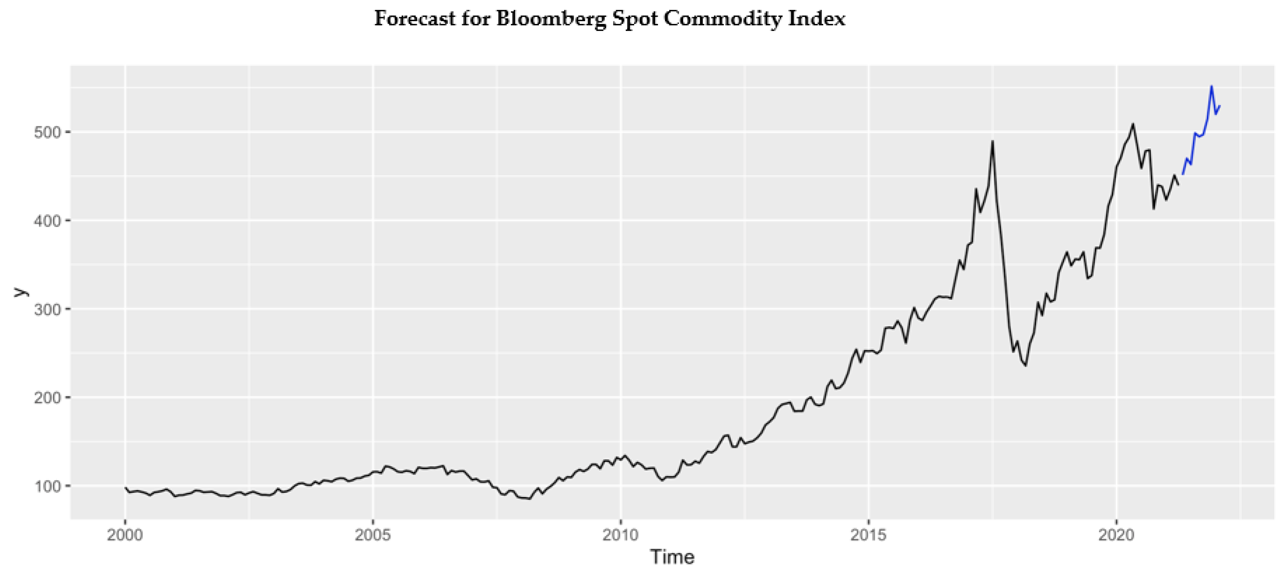
Finally, to corroborate the behavior of commodity prices (based on the fractional d parameter), following COVID-19, we have plotted the prices in Figure 5. In the charts, the black line represents the original time series, and the prediction in the next 10 periods (months) are represented in blue.
In our estimation, we assess the impact of SARS-CoV-2 on the Bloomberg Spot Commodity Index and its behavior in the next 10 months. These results are in line with the literature and other forecasts (see Štifanić et al. 2020; Kamdem et al. 2020; among others). According to our estimates, the Bloomberg Spot Commodity Index will recover its upward trend, rising from $338.37 in December 2019 to a price of $530.11 in February 2022, with the price increasing by 56.67% from before the start of the COVID-19 pandemic episode.
5. Concluding Comments
This research paper is relevant due to the paralysis, for several months, of the demand for raw materials, caused by SARS-CoV-2 and the ensuing lockdowns that were imposed throughout the world, which resulted in a collapse in prices. After the worst of the pandemic, the demand for industrial metals and other raw materials is recovering, spurred on by a new economic cycle and the new projects put in place already, or that are in the pipeline, for reforming infrastructures (Biden Administration in the United States, Recovery Funds in Europe, among others).
The main objective of this research work is to find out what impact COVID-19 has had on the prices of raw materials recorded in the Bloomberg Commodity Index from Thomson Reuters Eikon, observing how these alterations can influence the behavior of the economy in the coming quarters, and identifying the possible appearance of a new commodities supercycle in the wake of the 2020 health crisis. To this end, we analyze the statistical properties of these time series, measuring the degree of persistence, by using fractional integration techniques, to examine whether the impact of COVID-19 on the commodity prices is temporary or permanent. Moreover, the results have been supported by an Artificial Neural Network through the use of a Multilayer Perceptron (MLP) neural network for time series prediction. We examine the Bloomberg Spot Commodity Index and the Bloomberg Commodity Index Total Return, from 2 January 1991 to 2 April 2021, using monthly data.
Our first focus has been to analyze the statistical properties of these time series using several unit root methods, including ADF (Dickey and Fuller 1979), PP (Phillips and Perron 1988), and KPSS (Kwiatkowski et al. 1992). We get the results that the series are non-stationary I(1). Therefore, we have to calculate the first differences to make this time series stationary I(0).
We also used techniques based on fractional integration to know the degree of dependence of the series and to determine if the impact of COVID-19 on the commodity prices is temporary or permanent. We observe that both of the analyzed time series (the Bloomberg Spot Commodity Index and the Bloomberg Commodity Index Total Return) have the same behavior, observing that the I(0) Hypothesis cannot be rejected in the cases of the first recession in the United States or the SARS or MERS epidemic episodes, while for the second recession, this hypothesis is rejected in favor of a lower degree of integration. On the other hand, focusing on the COVID-19 episode, we observe that both time series have a mean reversion behavior, allowing us to speculate about the impact of SARS-CoV-2 on the Bloomberg Spot Commodity Index and its behavior in the next 12 months. These results are in line with the literature and other forecasts (see Štifanić et al. 2020; Kamdem et al. 2020; among others), and they are results by which it can be concluded that it is a temporary shock and, as such, it will not be necessary to implement additional measures, since the forecast is that the series will stabilize, returning to their long-term projections.
Finally, to corroborate the behavior of commodity prices (based on the fractional d parameter) after COVID-19, we use an Artificial Neural Networks (ANN) algorithm. In our forecast, we observe that the Bloomberg Spot Commodity Index will recover its upward trend; a price of $338.37 in December 2019, rose to a price of $530.11 in February 2022, with the price increasing by 56.67% since before the start of the COVID-19 pandemic episode. These results are, more or less, in line with the forecast presented in the research papers of the (Štifanić et al. 2020; Kamdem et al. 2020; among others).
A future line of research will be the verification of the results obtained by applying a Long Short Term Memory (LSTM) neural network (Hochreiter and Schmidhuber 1997), which is a type of RNN. The main characteristic of this type of network is that the information can persist by introducing loops in the network diagram, so it will have the ability to remember previous states, use this information to decide which one will be next, and contrast these results with those obtained by the Support Vector Machine (SVM) algorithm, which allows the upper limit of the generalization error of the model to be minimized and the estimation of its parameters to be equivalent to the solution of a quadratic programming model with linear restrictions.
The recent war with Ukraine threatens further disruption of supply chains, as Russia and Ukraine are essential suppliers of raw materials and energy. Thus, the impact of this conflict is spreading to the world economy (Schiffling and Kanellos 2022). The study carried out by (Mbah and Wasum 2022) analyzes the economic impact of the 2022 Russia–Ukraine war on the global economy (World Bank Group 2022). Both studies reflect the increase in the price of raw materials, observed in the second quarter of 2022, after the start of the war, which opens an interesting new line of research that reflects the differences between the predictions prior to the conflict and the results of the conflict.
Author Contributions
Conceptualization, M.M. and A.L.; Data curation, M.M.; Funding acquisition, M.M.; Investigation, M.M. and A.L.; Methodology, M.M.; Resources, M.M.; Software, M.M.; Supervision, M.M.; Validation, M.M.; Visualization, M.M. and A.L.; Writing—original draft, M.M. and A.L.; Writing—review & editing, M.M. and A.L. All authors have read and agreed to the published version of the manuscript.
Funding
Manuel Monge is acknowledge support from an internal Project of the Universidad Francisco de Vitoria.
Institutional Review Board Statement
Not applicable.
Conflicts of Interest
The authors declare no conflict of interest.
| 1 | https://fredhelp.stlouisfed.org/fred/data/understanding-the-data/recession-bars/ (access date 25 April 2021). |
| 2 | https://www.who.int/csr/don/2004_05_18a/en/ (access date on 25 April 2021). |
| 3 | A point of caution should be adopted here since the AIC and BIC may not necessarily be the best criteria for applications involving fractional models (Hosking 1981). |
References
- Adekoya, Oluwasegun B., and Johnson A. Oliyide. 2020. How COVID-19 drives connectedness among commodity and financial markets: Evidence from TVP-VAR and causality-in-quantiles techniques. Resources Policy 70: 101898. [Google Scholar] [CrossRef] [PubMed]
- Akaike, Htrotugu. 1973. Maximum likelihood identification of Gaussian autoregressive moving average models. Biometrika 60: 255–65. [Google Scholar] [CrossRef]
- Akaike, Hirotugu. 1979. A Bayesian extension of the minimum AIC procedure of autoregressive model fitting. Biometrika 66: 237–42. [Google Scholar] [CrossRef]
- Akhtaruzzaman, Md, Sabri Boubaker, and Ahmet Sensoy. 2021a. Financial contagion during COVID–19 crisis. Finance Research Letters 38: 101604. [Google Scholar] [CrossRef]
- Akhtaruzzaman, Md, Sabri Boubaker, Brian M. Lucey, and Ahmet Sensoy. 2021b. Is gold a hedge or safe haven asset during COVID19 crisis? Economic Modelling. [Google Scholar] [CrossRef]
- Akhtaruzzaman, Md, Sabri Boubaker, Mardy Chiah, and Angel Zhong. 2020. COVID-19 and oil price risk exposure. Finance Research Letters 42: 101882. [Google Scholar] [CrossRef]
- Arana, Estanislao, Martí-Bonmatí Luis, D. Bautista, and Paredes Roberto. 2003. Diagnóstico de las lesiones de la calota. Selección de variables por redes neuronales y regresión logística. Neurocirugía 14: 377–84. [Google Scholar] [CrossRef]
- Arbib, Michael A. 1995. Brain Theory and Neural Networks. Cambridge: MIT Press. [Google Scholar]
- Arbib, Michael A., Péter Érdi, and János Szentágothai. 1997. Neural Organization. Cambridge: MIT Press. [Google Scholar]
- Aslam, Faheem, Saqib Aziz, Duc Khuong Nguyen, Khurrum S. Mughal, and Maaz Khan. 2020. On the efficiency of foreign exchange markets in times of the COVID-19 pandemic. Technological Forecasting and Social Change 161: 120261. [Google Scholar] [CrossRef]
- Atsalakis, George S., and Kimon P. Valavanis. 2009. Surveying stock market forecasting techniques—Part II: Soft computing methods. Expert Systems with Applications 36: 5932–41. [Google Scholar] [CrossRef]
- Banerjee, Ameet Kumar. 2021. Futures market and the contagion effect of COVID-19 syndrome. Finance Research Letters 43: 102018. [Google Scholar] [CrossRef]
- Barkoulas, John T., Walter C. Labys, and Joseph I. Onochie. 1999. Long memory in futures prices. Financial Review 34: 91–100. [Google Scholar] [CrossRef]
- Barrow, Devon K., and Sven F. Crone. 2016. Cross-validation aggregation for combining autoregressive neural network forecasts. International Journal of Forecasting 32: 1120–37. [Google Scholar] [CrossRef] [Green Version]
- Ceballos, Francisco, Samyuktha Kannan, and Berber Kramer. 2020. Impacts of a national lockdown on smallholder farmers’ income and food security: Empirical evidence from two states in India. World Development 136: 105069. [Google Scholar] [CrossRef]
- Chen, Shyi-Ming, and Kurniawan Tanuwijaya. 2011. Multivariate fuzzy forecasting based on fuzzy time series and automatic clustering techniques. Expert Systems with Applications 38: 10594–605. [Google Scholar] [CrossRef]
- Christiano, Lawrence J., and Terry J. Fitzgerald. 2003. The Band Pass Filter. International Economic Review 44: 435–65. [Google Scholar] [CrossRef]
- Clavijo-Cortes, Pedro, Jacobo Campo Robledo, and Henry Antonio Mendoza Tolosa. 2020. Threshold effects and unit roots of real commodity prices since the mid-nineteenth century. Economics and Business Letters 9: 342–49. [Google Scholar] [CrossRef]
- Coakley, Jerry, Jian Dollery, and Neil Kellard. 2011. Long memory and structural breaks in commodity futures markets. Journal of Futures Markets 31: 1076–113. [Google Scholar] [CrossRef]
- Corbet, Shaen, John W. Goodell, and Samet Günay. 2020. Co-movements and spillovers of oil and renewable firms under extreme conditions: New evidence from negative WTI prices during COVID-19. Energy Economics 92: 104978. [Google Scholar] [CrossRef]
- Coulombe, Philippe Goulet, Maxime Leroux, Dalibor Stevanovic, and Stéphane Surprenant. 2020. How is machine learning useful for macroeconomic forecasting? arXiv arXiv:2008.12477. [Google Scholar] [CrossRef]
- Cox, John C., Jonathan E. Ingersoll Jr., and Stephen A. Ross. 1981. The relation between forward prices and futures prices. Journal of Financial Economics 9: 321–46. [Google Scholar] [CrossRef]
- Cuddington, John, and Abdel Zellou. 2012. Is there evidence of super-cycles in crude oil prices? SPE Economics and Management 4: 171–81. [Google Scholar]
- de Lillo, Antonio, and Cinzia Meraviglia. 1998. The role of social determinants on men’s and women’s mobility in Italy. A comparison of discriminant analysis and artificial neural networks. Substance Use & Misuse 33: 751–64. [Google Scholar]
- Deaton, Angus, and Guy Laroque. 1995. Estimating a Nonlinear Rational Expectations Commodity Price Model with Unobservable State Variables. Journal of Applied Econometrics 10: S9–S40. [Google Scholar] [CrossRef]
- Dickey, David A., and Wayne A. Fuller. 1979. Distributions of the estimators for autoregressive time series with a unit root. Journal of American Statistical Association 74: 427–81. [Google Scholar]
- Diebold, Francis, and Glen Rudebush. 1991. On the power of Dickey-Fuller tests against fractional alternatives. Economics Letters 35: 155–60. [Google Scholar] [CrossRef]
- Dittmann, Ingolf, and Clive W. J. Granger. 2002. Properties of nonlinear transformations of fractionally integrated processes. Journal of Econometrics 110: 113–33. [Google Scholar] [CrossRef] [Green Version]
- El-Henawy, Ibrahim Mahmoud, Kamal Hala, Hassan Abbas Abdelbary, and Ahmed R. Abas. 2010. Predicting stock index using neural network combined with evolutionary computation methods. Paper presented at 2010 The 7th International Conference on Informatics and Systems (INFOS), Cairo, Egypt, March 28–30; pp. 1–6. [Google Scholar]
- Elliott, Graham, Thomas J. Rothenberg, and James H. Stock. 1996. Efficient Tests for an Autoregressive Unit Root. Econometrica 64: 813–36. [Google Scholar] [CrossRef] [Green Version]
- Erdem, Fatma Pınar, and İbrahim Ünalmış. 2016. Revisiting super-cycles in commodity prices. Central Bank Review 16: 137–42. [Google Scholar] [CrossRef]
- Erten, Bilge, and José Antonio Ocampo. 2013. Super Cycles of Commodity Prices Since the Mid-Nineteenth Century. World Development 44: 14–30. [Google Scholar] [CrossRef] [Green Version]
- Erten, Bilge, and José Antonio Ocampo. 2021. The future of commodity prices and the pandemic-driven global recession: Evidence from 150 years of data. World Development 137: 105164. [Google Scholar] [CrossRef] [PubMed]
- Fassas, Athanasios P. 2020. Risk aversion connectedness in developed and emerging equity markets before and after the COVID-19 pandemic. Heliyon 6: e05715. [Google Scholar] [CrossRef] [PubMed]
- Fu, Li-Ming. 1994. Neural Networks in Computer Intelligence. New York: McGraw-Hill. [Google Scholar]
- Fuller, Wayne A. 1976. Introduction to Statistical Time Series. Fuller Introduction to Statistical Time Series 1976; New York: JohnWiley. [Google Scholar]
- Garbade, Kenneth D., and William L. Silber. 1983. Price Movement and Price Discovery in Futures and Cash Markets. The Review of Economics and Statistics 65: 289–97. [Google Scholar] [CrossRef]
- García, Ignacio, Alonso Marbán, Yenisse M. Tenorio, and José G. Rodriguez. 2008. Pronóstico de la Concentración de oxono en Guadalajara-México usando redes neuronales artificiales. Revista Información Tecnológica 19: 89–96. [Google Scholar]
- Geweke, John, and Susan Porter-Hudak. 1983. The estimation and application of long memory time series models. Journal of Time Series Analysis 4: 221–38. [Google Scholar] [CrossRef]
- Gholamy, Afshin, Vladik Kreinovich, and Olga Kosheleva. 2018. Why 70/30 or 80/20 Relation Between Training and Testing Sets: A Pedagogical Explanation. Available online: https://scholarworks.utep.edu/cs_techrep/1209/ (accessed on 15 May 2022).
- Gil-Alana, Luis A., Juncal Cunado, and Fernando Pérez de Gracia. 2012. Persistence, long memory, and unit roots in commodity prices. Canadian Journal of Agricultural Economics/Revue Canadienne D’agroeconomie 60: 451–68. [Google Scholar] [CrossRef]
- Glorot, Xavier, and Yoshua Bengio. 2010. Understanding the difficulty of training deep feedforward neural networks. Proceedings of the Thirteenth International Conference on Artificial Intelligence and Statistics. Proceedings of Machine Learning Research 9: 249–56. [Google Scholar]
- Glorot, Xavier, Antoine Bordes, and Yoshua Bengio. 2011. Domain Adaptation for Large-Scale Sentiment Classification: A Deep Learning Approach. In Proc. of ICML. pp. 513–20. Available online: http://dblp.unitrier.de/rec/bib/conf/icml/GlorotBB11 (accessed on 12 May 2022).
- Goolsbee, Austan, and Chad Syverson. 2020. Fear, lockdown, and diversion: Comparing drivers of pandemic economic decline 2020. Journal of Public Economics 193: 104311. [Google Scholar] [CrossRef]
- Granger, Clive William John, and Roselyne Joyeux. 1980. An introduction to long-memory time series models and fractional differencing. Journal of Time Series Analysis 1: 15–29. [Google Scholar] [CrossRef]
- Güler, Inan, and Elif Derya Übeyli. 2005. Adaptive neuro-fuzzy inference system for classification of EEG signals using wavelet coefficients. Journal of Neuroscience Methods 148: 113–21. [Google Scholar] [CrossRef]
- Haidar, Imad, Siddhivinayak Kulkarni, and Heping Pan. 2008. Forecasting model for crude oil prices based on artificial neural networks. Paper presented at International Conference on Intelligent Sensors, Sensor Networks and Information Processing, Sydney, NSW, Australia, December 15–18; pp. 103–08. [Google Scholar]
- Hassler, Uwe, and Jürgen Wolters. 1994. On the power of unit root tests against fractional alternatives. Economics Letters 45: 1–5. [Google Scholar] [CrossRef]
- Hinton, Geoffrey E., and Ruslan R. Salakhutdinov. 2006. Reducing the dimensionality of data with neural networks. Science 313: 504–7. [Google Scholar] [CrossRef] [PubMed] [Green Version]
- Hochreiter, Sepp, and Jürgen Schmidhuber. 1997. Long short-term memory. Neural Computation 9: 1735–80. [Google Scholar] [CrossRef] [PubMed]
- Holt, Matthew T., and Lee A. Craig. 2006. Nonlinear Dynamics and Structural Change in the U.S. Hog–Corn Cycle: A Time-Varying STAR Approach. American Journal of Agricultural Economics 88: 215–33. [Google Scholar] [CrossRef]
- Hosking, Jonathan Richard Morley. 1981. Fractional differencing. Biometrika 68: 165–76. [Google Scholar] [CrossRef]
- Hui, David S., Esam I. Azhar, Tariq A. Madani, Francine Ntoumi, Richard Kock, Osman Dar, Giuseppe Ippolito, Timothy D. Mchugh, Ziad A. Memish, Christian Drosten, and et al. 2020. The continuing 2019-nCoV epidemic threat of novel coronaviruses to global health—The latest 2019 novel coronavirus outbreak in Wuhan, China. International Journal of Infectious Diseases 91: 264–66. [Google Scholar] [CrossRef] [Green Version]
- Jacks, David S. 2013. From Boom to Bust: A Typology of Real Commodity Prices in the Long Run. Cliometrica 13: 201–20. [Google Scholar] [CrossRef] [Green Version]
- Jacks, David S., and Martin Stuermer. 2020. What drives commodity price booms and busts? Energy Economics 85: 104035. [Google Scholar] [CrossRef]
- Jadevicius, Arvydas, Brian Sloan, and Andrew Brown. 2010. A Century of research on property cycles—A review of research on major and auxiliary business cycles. International Journal of Strategic Property Management 21: 129–43. [Google Scholar] [CrossRef] [Green Version]
- James, Nick, Max Menzies, and Jennifer Chan. 2021. Changes to the extreme and erratic behaviour of cryptocurrencies during COVID-19. Physica A: Statistical Mechanics and Its Applications 565: 125581. [Google Scholar] [CrossRef]
- Jarrett, Kevin, Koray Kavukcuoglu, Marc’Aurelio Ranzato, and Yann LeCun. 2009. What is the best multi-stage architecture for object recognition? Paper presented at 2009 IEEE 12th International Conference on Computer Vision, Kyoto, Japan, September 29–October 2; pp. 2146–53. [Google Scholar]
- Jarrow, Robert A., and George S. Oldfield. 1981. Forward contracts and futures contracts. Journal of Financial Economics 9: 373–82. [Google Scholar] [CrossRef]
- Juglar, Clement. 1889. Des crises commerciales et leur retour périodique en France, en Angleterre et aux États-Units. Paris Alcan, Second Edition. Available online: https://gallica.bnf.fr/ark:/12148/bpt6k96055365.texteImage (accessed on 12 May 2022).
- Just, Małgorzata, and Krzysztof Echaust. 2020. Stock market returns, volatility, correlation and liquidity during the COVID-19 crisis: Evidence from the Markov switching approach. Finance Research Letters 37: 101775. [Google Scholar] [CrossRef] [PubMed]
- Kamdem, Jules Sadefo, Rose Bandolo Essomba, and James Njong Berinyuy. 2020. Deep learning models for forecasting and analyzing the implications of COVID-19 spread on some commodities markets volatilities. Chaos, Solitons & Fractals 140: 110215. [Google Scholar]
- Kellard, Neil, Paul Newbold, Tony Rayner, and Christine Ennew. 1999. The relative efficiency of commodity futures markets. The Journal of Futures Markets 19: 413–32. [Google Scholar] [CrossRef]
- Kilian, Lutz. 2009. Not all oil price shocks are alike: Disentangling demand and supply shocks in the crude oil market. American Economic Review 99: 1053–69. [Google Scholar] [CrossRef] [Green Version]
- Kondratiev, Nikolai D. 1925. The Major Economic Cycles. Moscow. Schumpeter’s business cycles. American Economic Review 30: 262–63. [Google Scholar]
- Kulkarni, Siddhivinayak, and Imad Haidar. 2009. Forecasting model for crude oil price using artificial neural networks and commodity futures prices. arXiv arXiv:0906.4838. [Google Scholar]
- Kuznets, Simon. 1940. Schumpeter’s Business Cycles. The American Economic Review 30: 257–71. [Google Scholar]
- Kwiatkowski, Denis, Peter C. B. Phillips, Peter Schmidt, and Yongcheol Shin. 1992. Testing the null hypothesis of stationarity against the alternative of a unit root. Journal of Econometrics 54: 159–78. [Google Scholar] [CrossRef]
- Lee, Dongin, and Peter Schmidt. 1996. On the power of the KPSS test of stationarity against fractionally-integrated alternatives. Journal of Econometrics 73: 285–302. [Google Scholar] [CrossRef]
- Li, Yuhong, and Weihua Ma. 2010. Application of artificial neural networks in financial economics: A survey. International Symposium on Computational Intelligence and Design 1: 211–14. [Google Scholar]
- Lien, Donald, and Yiu Kuen Tse. 1999. Fractional cointegration and futures hedging. Journal of Futures Markets 19: 457–74. [Google Scholar] [CrossRef]
- Mandelbrot, Benoit B. 1977. The Fractal Geometry of the Nature. New York: Freeman. [Google Scholar]
- Mapuwei, Tichaona W., Oliver Bodhlyera, and Henry Mwambi. 2020. Univariate Time Series Analysis of Short-Term Forecasting Horizons Using Artificial Neural Networks: The Case of Public Ambulance Emergency Preparedness. Journal of Applied Mathematics, 1–11. [Google Scholar] [CrossRef]
- Marshall, Alfred. 1890. Principles of Economics. London: Macmillan. [Google Scholar]
- Mbah, Ruth Endam, and Divine Forcha Wasum. 2022. Russian-Ukraine 2022 War: A review of the economic impact of Russian-Ukraine crisis on the USA, UK, Canada, and Europe. Advances in Social Sciences Research Journal 9: 144–53. [Google Scholar] [CrossRef]
- Mensi, Walid, Ahmet Sensoy, Xuan Vinh Vo, and Sang Hoon Kang. 2020. Impact of COVID-19 outbreak on asymmetric multifractality of gold and oil prices. Resources Policy 69: 101829. [Google Scholar] [CrossRef]
- Monge, Manuel, and Luis A. Gil-Alana. 2021. Lithium industry and the US crude oil prices. A Fractional Cointegration VAR and a Continuous Wavelet Transform analysis. Resources Policy 72: 102040. [Google Scholar] [CrossRef]
- Manuel, Monge, and Carlos Poza. 2021. Forecasting Spanish economic activity in times of COVID-19 by means of the RT-LEI and machine learning techniques. Working paper. Applied Economics Letters 1–6. [Google Scholar] [CrossRef]
- Nair, Vinod, and Geoffrey E. Hinton. 2010. Rectified linear units improve restricted boltzmann machines. In ICML. Available online: https://icml.cc/Conferences/2010/papers/432.pdf (accessed on 11 May 2022).
- Narayan, Paresh Kumar, Dinh Hoang Bach Phan, and Guangqiang Liu. 2020. COVID-19 lockdowns, stimulus packages, travel bans, and stock returns. Finance Research Letters 38: 101732. [Google Scholar] [CrossRef]
- Ng, Serena, and Pierre Perron. 2001. Lag length selection and the construction of unit root tests with good size and power. Econometrica 69: 1519–54. [Google Scholar] [CrossRef] [Green Version]
- Papadamou, Stephanos, Athanasios P. Fassas, Dimitris Kenourgios, and Dimitrios Dimitriou. 2020. Flight-to-quality between global stock and bond markets in the COVID era. Finance Research Letters 38: 101852. [Google Scholar] [CrossRef]
- Pedreira, Eduardo, and Canela Miguel-Angel. 2012. Modelling dependence in Latin American markets using copula functions. Journal of Emerging Market Finance 11: 231–70. [Google Scholar]
- Phillips, Peter C. B. 1987. Time series regression with a unit root. Econometrica 55: 277–301. [Google Scholar] [CrossRef]
- Phillips, Peter C. B. 1999. Discrete Fourier Transforms of Fractional Processes. Auckland: Department of Economics, University of Auckland. [Google Scholar]
- Phillips, Peter C. B. 2007. Unit root log periodogram regression. Journal of Econometrics 138: 104–24. [Google Scholar] [CrossRef] [Green Version]
- Phillips, Peter C. B., and Pierre Perron. 1988. Testing for a unit root in time series regression. Biometrika 75: 335–46. [Google Scholar] [CrossRef]
- Pindyck, Robert S. 2004. Volatility and commodity price dynamics. Journal of Futures Markets 24: 1029–47. [Google Scholar] [CrossRef] [Green Version]
- Radetzki, Marian. 2006. The anatomy of three commodity booms Resour. Policy 36: 56–64. [Google Scholar]
- Richard, Scott F., and Mahadevan Sundaresan. 1981. A continuous time equilibrium model of forward prices and futures prices in a multigood economy. Journal of Financial Economics 9: 347–71. [Google Scholar] [CrossRef]
- Robinson, Peter M. 1994. Efficient tests of nonstationary hypotheses. Journal of the American Statistical Association 89: 1420–37. [Google Scholar] [CrossRef]
- Robinson, Peter M. 1995a. Gaussian semi-parametric estimation of long range dependence. Annals of Statistics 23: 1630–61. [Google Scholar] [CrossRef]
- Robinson, Peter M. 1995b. Log periodogram regression of time series with long range dependence. Annals of Statistics 23: 1048–72. [Google Scholar] [CrossRef]
- Rumelhart, David E., George E. Hinton, and Ronald J. Williams. 1986. Learning representations by back-propagating errors. Nature 323: 533–36. [Google Scholar] [CrossRef]
- Salisu, Afees A., Godday U. Ebuh, and Nuruddeen Usman. 2020. Revisiting oil-stock nexus during COVID-19 pandemic: Some preliminary results. International Review of Economics & Finance 69: 280–94. [Google Scholar]
- Sanchez, Fernando, de Cos Juez, Francisco Javier, Ana Sánchez, Alicja Krzemień, and Pedro Fernández. 2015. Forecasting the COMEX copper spot price by means of neural networks and ARIMA models. Resources Policy 45: 37–43. [Google Scholar] [CrossRef]
- Schiffling, Sarah, and Nikolaos Valantasis Kanellos. 2022. Five essential commodities that will be hit by war in Ukraine. The Conversation. Available online: https://researchonline.ljmu.ac.uk/id/eprint/16422/1/Five%20essential%20commodities%20that%20will%20be%20hit%20by%20war%20in%20Ukraine.pdf (accessed on 15 May 2022).
- Sharif, Arshian, Chaker Aloui, and Larisa Yarovaya. 2020. COVID-19 pandemic, oil prices, stock market, geopolitical risk and policy uncertainty nexus in the US economy: Fresh evidence from the wavelet-based approach. International Review of Financial Analysis 70: 101496. [Google Scholar] [CrossRef]
- Simpson, Patrick K., and Thomas M. Brotherton. 1995. Fuzzy neural network machine prognosis. In Applications of Fuzzy Logic Technology II. Orlando: International Society for Optics and Photonics, vol. 2493, pp. 21–27. [Google Scholar]
- So, Mike K. P., Amanda M. Y. Chu, and Thomas W. C. Chan. 2021. Impacts of the COVID-19 pandemic on financial market connectedness. Finance Research Letters 38: 101864. [Google Scholar]
- Sowell, Fallaw. 1992. Maximum likelihood estimation of stationary univariate fractionally integrated time series models. Journal of Econometrics 53: 165–88. [Google Scholar] [CrossRef]
- Stein, Jerome L. 1961. The simultaneous determination of spot and future prices. American. Economic Review 51: 1012–25. [Google Scholar]
- Štifanić, Daniel, Jelena Musulin, Adrijana Miočević, Sandi Baressi Šegota, Roman Šubić, and Zlatan Car. 2020. Impact of COVID-19 on forecasting stock prices: An integration of stationary wavelet transform and bidirectional long short-term memory. Complexity 2020: 1846926. Available online: https://www.hindawi.com/journals/complexity/2020/1846926/ (accessed on 13 February 2022).
- Taud, Hind, and J. F. Mas. 2018. Multilayer Perceptron (MLP). In Geomatic Approaches for Modeling Land Change Scenarios. Lecture Notes in Geoinformation and Cartography. Edited by Maria Camacho Olmedo, Martin Paegelow, Jean Francois Mas and Francisco Escobar. Cham: Springer. [Google Scholar]
- Trippi, Robert R., and Efraim Turban. 1996. Neural Networks in Finance and Investing. Edición Revisada, 821. New York: McGraw Hill, Nueva York, Estados Unidos. [Google Scholar]
- Villada, Fernando, Edwin García, and Juan D. Molina. 2011. Pronóstico del precio de la energía eléctrica usando redes neuro-difusas. Revista Información Tecnológica 22: 111–20. [Google Scholar] [CrossRef]
- Villada, Fernando, Nicolás Muñoz, and Edwin García. 2012. Aplicación de las Redes Neuronales al Pronóstico de Precios en el Mercado de Valores. Información Tecnológica 23: 11–20. [Google Scholar] [CrossRef] [Green Version]
- Wang, Dabin, and William G. Tomek. 2007. Commodity Prices and Unit Root Tests. American Journal of Agricultural Economics 89: 873–89. [Google Scholar] [CrossRef]
- World Bank Group. 2022. Commodity Markets Outlook: The Impact of the War in Ukraine on Commodity Markets, April 2022. License: Creative Commons Attribution CC BY 3.0 IGO. Washington, DC: World Bank. [Google Scholar]
- Zhang, Aston, Zachary C. Lipton, Mu Li, and Alexander J. Smola. 2020. Dive into Deep Learning. arXiv arXiv:2106.11342. [Google Scholar]
Figure 1.
Percent change in commodity prices (1 January 2020–1 May 2021). Source: https://el–ments.visualcapitalist.com/visualizing-the-rise-in-commodity-prices/, (access date on 25 April 2021).
Figure 1.
Percent change in commodity prices (1 January 2020–1 May 2021). Source: https://el–ments.visualcapitalist.com/visualizing-the-rise-in-commodity-prices/, (access date on 25 April 2021).

Figure 2.
Crude Oil prices: West Texas Intermediate. Source: U.S. Energy Information Administration, Crude Oil Prices: West Texas Intermediate (WTI)—Cushing, Oklahoma [DCOILWTICO].
Figure 2.
Crude Oil prices: West Texas Intermediate. Source: U.S. Energy Information Administration, Crude Oil Prices: West Texas Intermediate (WTI)—Cushing, Oklahoma [DCOILWTICO].

Figure 3.
Bloomberg Commodity Index.

Figure 4.
Artificial Neural Network for time series forecasting.

Figure 5.
Forecast after the COVID-19 structural break in the commodity index.


Table 1.
Periods analyzed.
| Table 1: U.S. Recessions | ||
| 1st period | 1 March 2001 | 2 November 2001 |
| 2nd period | 2 December 2007 | 2 June 2009 |
| Source: Federal Reserve Bank of St. Louis (https://fredhelp.stlouisfed.org/fred/data/understanding-the-data/recession-bars/, (access date on 25 April 2021)) | ||
| Pandemic, epidemic diseases | ||
| 3rd period | 2 November 2002 | 2 May 2004 |
| 4th period | 3 September 2012 | 2 April 2021 |
| 5th period | 2 December 2019 | 2 April 2021 |
| Source: World Health Organization | ||
Table 2.
Unit root tests.
| ADF | PP | KPSS | ||||||
|---|---|---|---|---|---|---|---|---|
| (i) | (ii) | (iii) | (ii) | (iii) | (ii) | (iii) | ||
| Original Time Series | ||||||||
| Bloomberg Spot Commodity Index | 0.6465 | −0.9047 | −2.1624 | −1.008 | −2.4171 | 5.1135 | 0.6113 | |
| Bloomberg Commodity Index Total Return | −0.3105 | −1.7857 | −1.5164 | −1.8792 | −1.6839 | 2.3298 | 1.152 | |
| U.S. Recession | ||||||||
| 1st period: Mar 2001–Nov 2001 | Bloomberg Spot Commodity Index | 0.1622 | −1.5137 | −1.5828 | −1.6433 | −1.7796 | 1.173 | 0.174 |
| Bloomberg Commodity Index Total Return | 0.6386 | −1.1752 | −1.5234 | −1.2505 | −1.693 | 1.8694 | 0.1527 | |
| 2nd period: Dec 2007–Jun 2009 | Bloomberg Spot Commodity Index | 0.4289 | −1.4341 | −2.3161 | −1.4816 | −2.2696 | 2.0018 | 0.1071 |
| Bloomberg Commodity Index Total Return | 0.0431 | −1.8668 | −1.5957 | −1.8815 | −1.5408 | 1.6018 | 0.2196 | |
| Pandemic, Epidemic diseases | ||||||||
| 3rd period: Nov 2002–May 2004 | Bloomberg Spot Commodity Index | 2.2295 | 1.7157 | 0.1609 | 1.8232 | −0.0636 | 2.0347 | 0.3185 |
| Bloomberg Commodity Index Total Return | 2.5927 | 1.3852 | −0.3832 | 1.4408 | −0.5891 | 2.5761 | 0.1875 | |
| 4th period: Sept 2012–Apr 2021 | Bloomberg Spot Commodity Index | −0.4646 | −1.9743 | −1.0244 | −1.9642 | −1.1442 | 0.6592 | 0.3453 |
| Bloomberg Commodity Index Total Return | −2.1408 | −2.5472 | −1.3201 | −2.2194 | −1.3748 | 1.6664 | 0.3902 | |
| 5th period: Dec 2019–Apr 2021 | Bloomberg Spot Commodity Index | 0.6697 | −0.2363 | −2.9693 | −0.2337 | −1.6612 | 0.4816 | 0.152 |
| Bloomberg Commodity Index Total Return | −0.0165 | −1.3443 | −2.8273 | −1.0219 | −1.4235 | 0.2797 | 0.1546 | |
(i) Refers to the model with no deterministic components; (ii) with an intercept; (iii) with a linear time trend. I reflect t-statistic with test critical value at 5%.
Table 3.
Results of long memory tests.
| Original Time Series | ||||||
|---|---|---|---|---|---|---|
| Data Analyzed | ARFIMA Model | d | Std. Error | Interval | I(d) | |
| Bloomberg Spot Commodity Index | ARFIMA (2, d, 2) | 0.618112 | 0.208399 | [0.28, 0.96] | I(d) | |
| Bloomberg Commodity Index Total Return | ARFIMA (2, d, 2) | 0.7368393 | 0.1563650 | [0.48, 0.99] | I(d) | |
| U.S. Recession periods | ||||||
| Period | Data Analyzed | ARFIMA model | d | Std. Error | Interval | I(d) |
| 1st period: Jan 1991–Nov 2001 | Bloomberg Spot Commodity Index | ARFIMA (2, d, 2) | 1.2852611 | 0.1965197 | [0.96, 1.61] | I(1) |
| Bloomberg Commodity Index Total Return | ARFIMA (1, d, 1) | 1.335611 | 0.161152 | [1.07, 1.60] | I(1) | |
| 2nd period: Dec 2007–Jun 2009 | Bloomberg Spot Commodity Index | ARFIMA (2, d, 2) | 0.08692761 | 0.31085366 | [−0.42, 0.60] | I(0) |
| Bloomberg Commodity Index Total Return | ARFIMA (2, d, 2) | 0.2668279 | 0.3982462 | [−0.39, 0.92] | I(0) | |
| Pandemic, Epidemic diseases | ||||||
| 3rd period: Nov 2002–May 2004 | Bloomberg Spot Commodity Index | ARFIMA (1, d, 1) | 1.283334 | 0.162049 | [1.02, 1.55] | I(1) |
| Bloomberg Commodity Index Total Return | ARFIMA (1, d, 1) | 1.323594 | 0.151526 | [1.07, 1.57] | I(1) | |
| 4th period: Sept 2012–Apr 2021 | Bloomberg Spot Commodity Index | ARFIMA (0, d, 1) | 1.1489924 | 0.1374773 | [0.92, 1.38] | I(1) |
| Bloomberg Commodity Index Total Return | ARFIMA (0, d, 1) | 1.126025 | 0.137913 | [0.90, 1.35] | I(1) | |
| 5th period: Dec 2019–Apr 2021 | Bloomberg Spot Commodity Index | ARFIMA (2, d, 1) | 0.5139049 | 0.4956813 | [−0.30, 1.33] | I(0), I(1) |
| Bloomberg Commodity Index Total Return | ARFIMA (2, d, 1) | 0.5100576 | 0.5038849 | [−0.32, 1.34] | I(0), I(1) | |
Table 4.
Forecast results and accuracies of the time series of commodity prices, after a structural break, using the ANN model.
Table 4.
Forecast results and accuracies of the time series of commodity prices, after a structural break, using the ANN model.
| Bloomberg Spot Commodity Index | |
|---|---|
| Spot price of BSCI (3 February 2022) | 559.03$ |
| Result obtained in our forecast | 530.11$ |
| MSE of the ANN model | 0.0005 |
| Deviation from spot price | 0.0517 |
Publisher’s Note: MDPI stays neutral with regard to jurisdictional claims in published maps and institutional affiliations. |
© 2022 by the authors. Licensee MDPI, Basel, Switzerland. This article is an open access article distributed under the terms and conditions of the Creative Commons Attribution (CC BY) license (https://creativecommons.org/licenses/by/4.0/).
Share and Cite
MDPI and ACS Style
Monge, M.; Lazcano, A. Commodity Prices after COVID-19: Persistence and Time Trends. Risks 2022, 10, 128. https://doi.org/10.3390/risks10060128
AMA Style
Monge M, Lazcano A. Commodity Prices after COVID-19: Persistence and Time Trends. Risks. 2022; 10(6):128. https://doi.org/10.3390/risks10060128
Chicago/Turabian StyleMonge, Manuel, and Ana Lazcano. 2022. "Commodity Prices after COVID-19: Persistence and Time Trends" Risks 10, no. 6: 128. https://doi.org/10.3390/risks10060128
Note that from the first issue of 2016, this journal uses article numbers instead of page numbers. See further details here.